 Rui Guo1
95% of researchers rate our articles as excellent or good
Learn more about the work of our research integrity team to safeguard the quality of each article we publish.
Find out more
ORIGINAL RESEARCH article
Front. Phys. , 25 January 2022
Sec. Interdisciplinary Physics
Volume 9 - 2021 | https://doi.org/10.3389/fphy.2021.791858
This article is part of the Research Topic Long-Range Dependent Processes: Theory and Applications View all 15 articles
In this study, as a continuation to the studies of the self-interaction diffusion driven by subfractional Brownian motion SH, we analyze the asymptotic behavior of the linear self-attracting diffusion:
where θ > 0 and
In a previous study (I) (see [12]), as an extension to classical result, we considered the linear self-interacting diffusion as follows:
with θ ≠ 0, where θ and ν are two real numbers, and SH is a sub-fBm with the Hurst parameter
and
in L2 and almost surely, for all n = 1, 2, …, where ( − 1)!! = 1 and
In the present study, we consider the case θ > 0 and study its large time behaviors.
Let us recall the main results concerning the system (Eq. 1). When
where B is a d-dimensional standard Brownian motion and f is Lipschitz continuity. Xt corresponds to the location of the end of the polymer at time t. Under some conditions, they established asymptotic behavior of the solution of the stochastic differential equation. The model is a continuous analog of the notion of edge (respectively, vertex) self-interacting random walk (see, e.g., Pemantle [22]). By using the local time of the solution process X, we can make it clear how the process X interacts with its own occupation density. In general, Eq. 2 defines a self-interacting diffusion without any assumption on f. We call it self-repelling (respectively, self-attracting) if, for all
In this present study, our main aim is to expound and prove the following statements:
(I) For θ > 0 and
exists as an element in L2, where the function is defined as follows:
with θ > 0.
(II) For θ > 0 and
in L2 and almost surely as t → ∞.
(III) For θ > 0 and
in distribution as t → ∞, where
(IV) For θ > 0 and
Then the convergence
holds in L2 as T tends to infinity.
This article is organized as follows. In Section 2, we present some preliminaries for sub-fBm and Malliavin calculus. In Section 3, we obtain some lemmas. In Section 4, we prove the main results given as before. In Section 5, we give some numerical results.
In this section, we briefly recall the definition and properties of stochastic integral with respect to sub-fBm. We refer to Alós et al [1], Nualart [21], and Tudor [31] for a complete description of stochastic calculus with respect to Gaussian processes.
As we pointed out in the previous study (I) (see [12]), the sub-fBm SH is a rather special class of self-similar Gaussian processes such that
for all s, t ≥ 0. For H = 1/2, SH coincides with the standard Brownian motion B. SH is neither a semimartingale nor a Markov process unless H = 1/2, so many of the powerful techniques from stochastic analysis are not available when dealing with SH. As a Gaussian process, it is possible to construct a stochastic calculus of variations with respect to SH. The sub-fBm appeared in Bojdecki et al [4] in a limit of occupation time fluctuations of a system of independent particles moving in
The normality and Hölder continuity of the sub-fBm SH imply that
as the limit in probability of a Riemann sum. Clearly, when u is of bounded qH variation on any finite interval with qH > 1 and
for all t ≥ 0.
Let
for s, t ∈ [0, T]. For every
as a linear (isometric) mapping from
for any
where
for s, t ∈ [0, T]. Thus, when
we can define the integral as follows:
and
Let now D and δ be the (Malliavin) derivative and divergence operators associated with the sub-fBm SH. And let
Then the duality relationship
holds for any
where (Du)∗ is the adjoint of Du in the Hilbert space given as follows:
for an adapted process u, and it is called the Skorohod integral. By using Alós et al [1], we can obtain the relationship between the Skorohod and the Young integral as follows:
provided u has a bounded q variation with
For simplicity, we throughout let C stand for a positive constant which depends only on its superscripts, and its value may be different in different appearances, and this assumption is also suitable to c. Recall that the linear self-attracting diffusion with sub-fBm SH is defined by the following stochastic differential equation:
with θ > 0. The kernel (t, s)↦hθ(t, s) is defined as follows:
for s, t ≥ 0. By the variation of constants method (see, Cranston and Le Jan [8]) or Itô’s formula, we may introduce the following representation:
for t ≥ 0.
The kernel function (t, s)↦hθ(t, s) with θ > 0 admits the following properties (these properties are proved partly in Cranston and Le Jan [8]):
• For all s ≥ 0, the limit
exists.
• For all t ≥ s ≥ 0, we have hθ(s) ≤ hθ(t, s), and
• For all t ≥ s, r ≥ 0 and θ ≠ 0, we have
and
• For all t > 0, we have
Lemma 3.1 Let
exists as an element in L2.
Proof This is a simple calculus exercise. In fact, we have
for all θ > 0 and
and
and
for all θ > 0 and
Lemma 3.2 Let θ > 0. We then have
Proof This is a simple calculus exercise. In fact, we have
for all t ≥ 0 and θ > 0. Noting that
and
we see that
by L’Hopital’s rule.
Lemma 3.3 Let θ > 0. We then have
for all t ≥ 0.
Lemma 3.4 Let θ > 0 and
Proof By L’Hopital’s rule and the change of variable
where we have used the equation
This completes the proof.
Lemma 3.5 Let θ > 0 and
for all 0 ≤ s < t ≤ T, where C and c are two positive constants depending only on H, θ, ν and T.
Proof The lemma is similar to Lemma 3.5 in the previous study (I).
Lemma 3.6 Let θ > 0 and
holds in L2 and almost surely as t tends to infinity.
Proof Convergence (18) in L2 follows from Lemma (3.1). In fact, by Eq. 10, we have
as t tends to infinity.On the other hand, by Lemma (3.5), 3.3 and the equation
as t tends to infinity. It follows from the integration by parts that
almost surely as t tends to infinity.
In this section, we consider the long time behaviors for XH with
Theorem 4.1 Let θ > 0 and
holds in L2 and almost surely as t tends to infinity.
Proof When
for all t ≥ 0.We first check that Eq. 19 holds in L2. By Lemma 3.6 and Lemma 3.2, we only need to prove
for all θ > 0 as t tends to infinity and Lemma 3.4 that
for all θ > 0 and
for all θ > 0 and
for every integer n ≥ 1. Then {Zn,k, k = 0, 1, 2, …, n} is Gaussian for every integer n ≥ 1. It follows from Lemma 3.4 that
for every integer n ≥ 1 and 0 ≤ k ≤ n, which implies that
for any ɛ > 0, every integer n ≥ 1 and 0 ≤ k ≤ n.On the other hand, for every s ∈ (0, 1), we denote
Then
for all s, s′ ∈ [0, 1]. Thus, for any ɛ > 0, by Slepian’s theorem and Markov’s inequality, one can get
for every integer n ≥ 1 and 0 ≤ k ≤ n. Combining this with the Borel–Cantelli lemma and the relationship
we show that
Theorem 4.2 Let θ > 0 and
holds in distribution, where
Proof When
in probability and
in distribution.First, Eq. 22 follows from Eq. 10 and
for all θ > 0 and
as t tends to infinity and Lemma 3.4, we get
for all θ > 0 and
Then the self-attracting diffusion XH satisfies
and
by integration by parts. It follows that
for all
Lemma 4.1 Let
almost surely and in L2 as T tends to infinity.
Proof This lemma follows from Eq. 24 and the estimates
as T tends to infinity.
Theorem 4.3 Let
in L2 as T tends to infinity.
Proof Given
for all t ≥ 0. Then
for all t ≥ 0. We now prove the lemma in three steps.
Step I We claim that
as t tends to infinity. Clearly, we have
Thus, 29 is equivalent to
By L’Hôspital’s rule and Lemma 3.4, it follows that
for all
Step II We claim that
as T tends to infinity. We have that
for all t > s > 0. An elementary calculation may show that
for all t > s > 0. It follows from the equation
for all t > s > 0 and 0 ≤ α ≤ 1. For the term Λ2(H; t, s), by the proof of Lemma 3.4, we find that
for all
and the equation
for all t > s > 0,
holds for all t > s ≥ 0. In particular, we have
for all t, s ≥ 0. As a corollary, we get
as T tends to infinity.
Step III We claim that
as t tends to infinity. By steps I and II, we find that Eq. 37 is equivalent to
as t tends to infinity. Noting that the equation
for all t, s > 0, we further find that convergence (38) also is equivalent to
as T tends to infinity. We now check that convergence (40) in two cases.
Case 1 Let
Case 2 Let
with
with
for all T > 1 and
with
as T tends to infinity. This shows that convergence (40) holds for all
Remark 1 By using the Borel–Cantelli lemma and Theorem 4.3, we can check that convergence (28) holds almost surely.
We have applied our results to the following linear self-attracting diffusion driven by a sub-fBm SH with
where θ > 0 and
• H = 0.7: θ = 1, θ = 10 and θ = 100, respectively (see, Figures 1–3, Tables 1–3);
• H = 0.5: θ = 1, θ = 10 and θ = 100, respectively (see, Figures 4–6, Tables 4–6).

FIGURE 1. Path of XH with θ = 1 and H = 0.7.
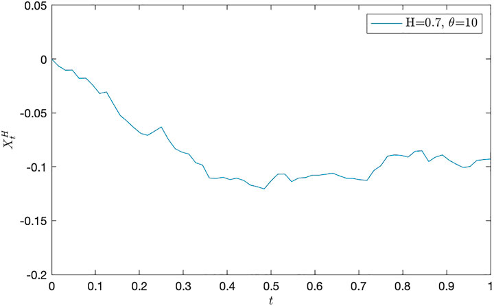
FIGURE 2. Path of XH with θ = 10 and H = 0.7.
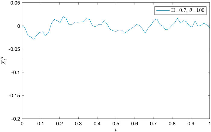
FIGURE 3. Path of XH with θ = 100 and H = 0.7.
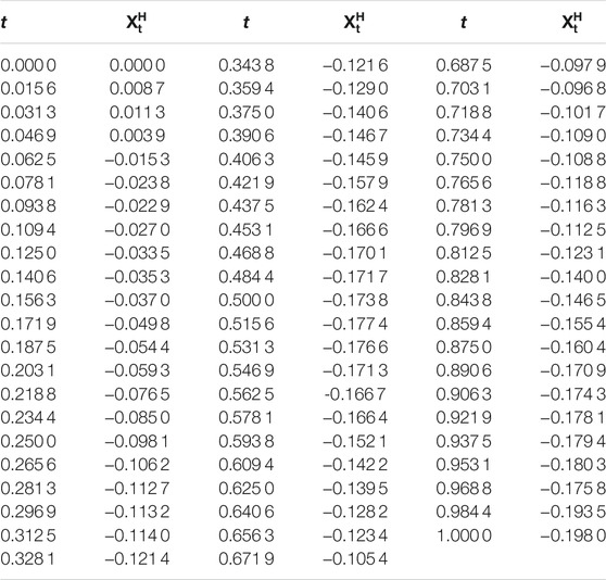
TABLE 1. Data of
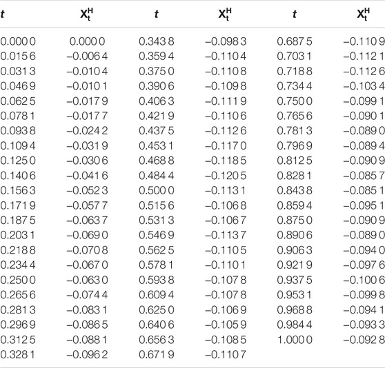
TABLE 2. Data of
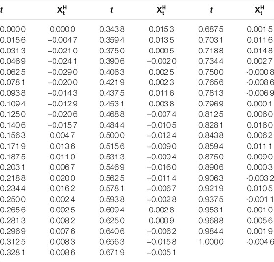
TABLE 3. Data of
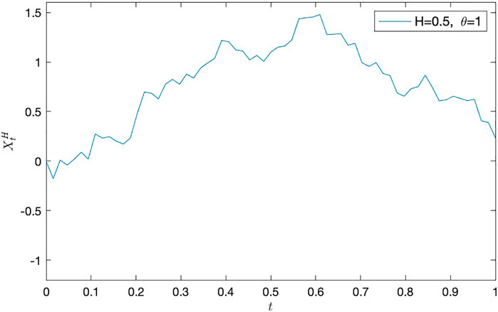
FIGURE 4. Path of XH with θ = 1 and H = 0.5.
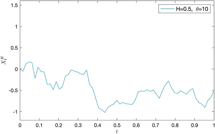
FIGURE 5. Path of XH with θ = 10 and H = 0.5.
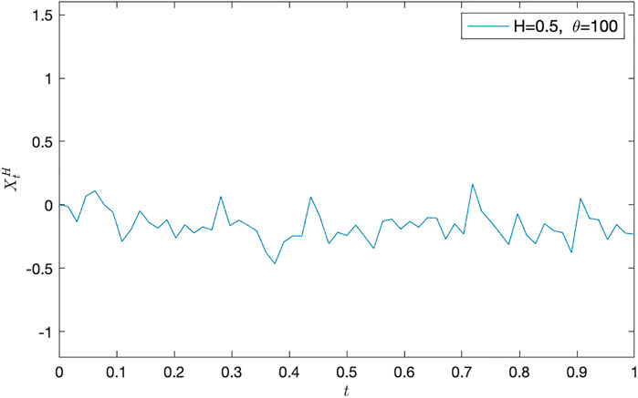
FIGURE 6. Path of XH with θ = 100 and H = 0.5.
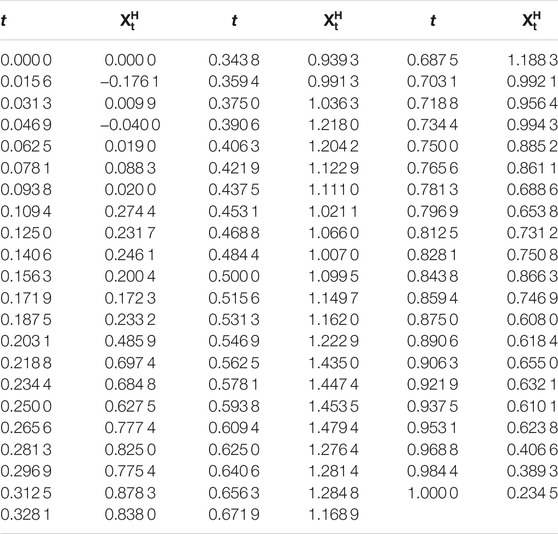
TABLE 4. Data of
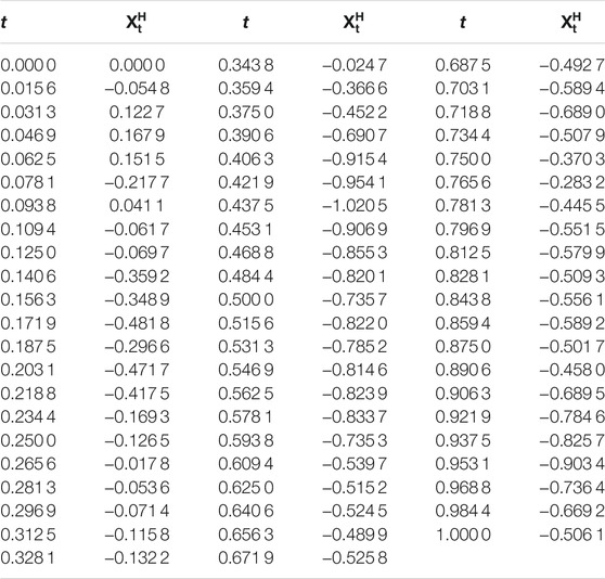
TABLE 5. Data of
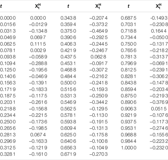
TABLE 6. Data of
Remark 2 From the following numerical results, we can find that it is important to study the estimates of parameters θ and ν.
The original contributions presented in the study are included in the article/supplementary material; further inquiries can be directed to the corresponding authors.
All authors listed have made a substantial, direct, and intellectual contribution to the work and approved it for publication.
The authors declare that the research was conducted in the absence of any commercial or financial relationships that could be construed as a potential conflict of interest.
All claims expressed in this article are solely those of the authors and do not necessarily represent those of their affiliated organizations, or those of the publisher, the editors, and the reviewers. Any product that may be evaluated in this article, or claim that may be made by its manufacturer, is not guaranteed or endorsed by the publisher.
1. Alós E, Mazet O, Nualart D Stochastic Calculus with Respect to Gaussian Processes. Ann Prob (2001) 29:766–801. doi:10.1214/aop/1008956692
2. Benaïm M, Ciotir I, Gauthier C-E Self-repelling Diffusions via an Infinite Dimensional Approach. Stoch Pde: Anal Comp (2015) 3:506–30. doi:10.1007/s40072-015-0059-5
3. Benaïm M, Ledoux M, Raimond O Self-interacting Diffusions. Probab Theor Relat Fields (2002) 122:1–41. doi:10.1007/s004400100161
4. Bojdecki T, Gorostiza LG, Talarczyk A Some Extensions of Fractional Brownian Motion and Sub-fractional Brownian Motion Related to Particle Systems. Elect Comm Probab (2007) 12:161–72. doi:10.1214/ecp.v12-1272
5. Bojdecki T, Gorostiza LG, Talarczyk A Sub-fractional Brownian Motion and its Relation to Occupation Times. Stat Probab Lett (2004) 69:405–19. doi:10.1016/j.spl.2004.06.035
6. Bojdecki T, Gorostiza LG, Talarczyk A Occupation Time Limits of Inhomogeneous Poisson Systems of Independent Particles. Stochastic Process their Appl (2008) 118:28–52. doi:10.1016/j.spa.2007.03.008
7. Bojdecki T, Gorostiza LG, Talarczyk A Self-Similar Stable Processes Arising from High-Density Limits of Occupation Times of Particle Systems. Potential Anal (2008) 28:71–103. doi:10.1007/s11118-007-9067-z
8. Cranston M, Le Jan Y Self Attracting Diffusions: Two Case Studies. Math Ann (1995) 303:87–93. doi:10.1007/bf01460980
9. Cranston M, Mountford TS The strong Law of Large Numbers for a Brownian Polymer. Ann Probab (1996) 24:1300–23. doi:10.1214/aop/1065725183
10. Durrett RT, Rogers LCG Asymptotic Behavior of Brownian Polymers. Probab Th Rel Fields (1992) 92:337–49. doi:10.1007/bf01300560
11. Gan Y, Yan L Least Squares Estimation for the Linear Self-Repelling Diffusion Driven by Fractional Brownian Motion (In Chinese). Sci CHINA Math (2018) 48:1143. doi:10.1360/scm-2017-0387
12.H Gao, R Guo, Y Jin, and L Yan, Large Time Behavior on the Linear Self-Interacting Diffusion Driven by Sub-fractional Brownian Motion I: Self-Repelling Case. Front Phys (2021) volume 2021. doi:10.3389/fphy.2021.795210
13. Gauthier C-E Self Attracting Diffusions on a Sphere and Application to a Periodic Case. Electron Commun Probab (2016) 21(No. 53):1–12. doi:10.1214/16-ecp4547
14. Herrmann S, Roynette B Boundedness and Convergence of Some Self-Attracting Diffusions. Mathematische Annalen (2003) 325:81–96. doi:10.1007/s00208-002-0370-0
15. Herrmann S, Scheutzow M Rate of Convergence of Some Self-Attracting Diffusions. Stochastic Process their Appl (2004) 111:41–55. doi:10.1016/j.spa.2003.10.012
16. Li M Modified Multifractional Gaussian Noise and its Application. Phys Scr (2021) 96(1212):125002. doi:10.1088/1402-4896/ac1cf6
17. Li M Generalized Fractional Gaussian Noise and its Application to Traffic Modeling. Physica A (2021) 579:126138. doi:10.1016/j.physa.2021.126138
18. Li M Multi-fractional Generalized Cauchy Process and its Application to Teletraffic. Physica A: Stat Mech its Appl (2020) 550(14):123982. doi:10.1016/j.physa.2019.123982
19. Li M Fractal Time Series-A Tutorial Review. Math Probl Eng (2010) 2010:1–26. doi:10.1155/2010/157264
20. Mountford T, Tarrés P An Asymptotic Result for Brownian Polymers. Ann Inst H Poincaré Probab Statist (2008) 44:29–46. doi:10.1214/07-aihp113
22. Pemantle R Phase Transition in Reinforced Random Walk and RWRE on Trees. Ann Probab (1988) 16:1229–41. doi:10.1214/aop/1176991687
23. Shen G, Yan L An Approximation of Subfractional Brownian Motion. Commun Stat - Theor Methods (2014) 43:1873–86. doi:10.1080/03610926.2013.769598
24. Shen G, Yan L Estimators for the Drift of Subfractional Brownian Motion. Commun Stat - Theor Methods (2014) 43:1601–12. doi:10.1080/03610926.2012.697243
25. Sun X, Yan L A central Limit Theorem Associated with Sub-fractional Brownian Motion and an Application (In Chinese). Sci Sin Math (2017) 47:1055–76. doi:10.1360/scm-2016-0748
26. Sun X, Yan L A Convergence on the Linear Self-Interacting Diffusion Driven by α-stable Motion. Stochastics (2021) 93:1186–208. doi:10.1080/17442508.2020.1869239
27. Sun X, Yan L The Laws of Large Numbers Associated with the Linear Self-Attracting Diffusion Driven by Fractional Brownian Motion and Applications, to Appear in. J Theoret Prob (2021). Online. doi:10.1007/s10959-021-01126-0
28. Tudor C Some Properties of the Sub-fractional Brownian Motion. Stochastics (2007) 79:431–48. doi:10.1080/17442500601100331
29. Tudor C Inner Product Spaces of Integrands Associated to Subfractional Brownian Motion. Stat Probab Lett (2008) 78:2201–9. doi:10.1016/j.spl.2008.01.087
30. Tudor C On the Wiener Integral with Respect to a Sub-fractional Brownian Motion on an Interval. J Math Anal Appl (2009) 351:456–68. doi:10.1016/j.jmaa.2008.10.041
31. Tudor C Some Aspects of Stochastic Calculus for the Sub-fractional Brownian Motion. Ann Univ Bucuresti Mathematica (2008) 24:199–230.
32. Tudor CA. Analysis of Variations for Self-Similar Processes. Heidelberg, New York: Springer (2013).
33. Yan L, He K, Chen C The Generalized Bouleau-Yor Identity for a Sub-fractional Brownian Motion. Sci China Math (2013) 56:2089–116. doi:10.1007/s11425-013-4604-2
34. Yan L, Sun Y, Lu Y On the Linear Fractional Self-Attracting Diffusion. J Theor Probab (2008) 21:502–16. doi:10.1007/s10959-007-0113-y
35. Yan L, Shen G On the Collision Local Time of Sub-fractional Brownian Motions. Stat Probab Lett (2010) 80:296–308. doi:10.1016/j.spl.2009.11.003
Keywords: subfractional Brownian motion, self-attracting diffusion, law of large numbers, Malliavin calculus, asymptotic distribution
Citation: Guo R, Gao H, Jin Y and Yan L (2022) Large Time Behavior on the Linear Self-Interacting Diffusion Driven by Sub-Fractional Brownian Motion II: Self-Attracting Case. Front. Phys. 9:791858. doi: 10.3389/fphy.2021.791858
Received: 09 October 2021; Accepted: 19 November 2021;
Published: 25 January 2022.
Edited by:
Ming Li, Zhejiang University, ChinaReviewed by:
Xiangfeng Yang, Linköping University, SwedenCopyright © 2022 Guo, Gao, Jin and Yan. This is an open-access article distributed under the terms of the Creative Commons Attribution License (CC BY). The use, distribution or reproduction in other forums is permitted, provided the original author(s) and the copyright owner(s) are credited and that the original publication in this journal is cited, in accordance with accepted academic practice. No use, distribution or reproduction is permitted which does not comply with these terms.
*Correspondence: Han Gao, 1061760802@qq.com
Disclaimer: All claims expressed in this article are solely those of the authors and do not necessarily represent those of their affiliated organizations, or those of the publisher, the editors and the reviewers. Any product that may be evaluated in this article or claim that may be made by its manufacturer is not guaranteed or endorsed by the publisher.
Research integrity at Frontiers
Learn more about the work of our research integrity team to safeguard the quality of each article we publish.