Investigating spatially varying relationships between the distribution of rural settlements and related influences

The distribution of rural settlements is a complex outcome of human adaptation to natural conditions and socioeconomic development throughout history. Scientifically revealing the spatially varying relationships between the distribution of rural settlements and the related factors is fundamental for effective planning and management. In this study, we focus on the North China Plain to analyze the spatially varying relationships between the distribution of rural settlements and the related factors using both traditional statistical and geographically weighted regression models. Our findings reveal that both the number and the area of rural settlements at the county level are increasing from north to south and from west to east. The results of the traditional regression model suggest that total area, total population, road density, precipitation, road length, slope, longitude, and temperature significantly influence the rural settlement area, while those influencing the number of rural settlements are longitude, latitude, road length, road density, river length, and river density. Moreover, the regression coefficients are constant in the global model, while both the magnitude and the sign of the corresponding parameters in the local model are spatially varying. However, the value of the coefficients in the global model are within the range of the coefficients in the local model and most coefficients in the local model share the same sign with that the global model. Our results also reveal that the local model outperforms the global model with the same explanatory variables, indicating a smaller Akaike’s information criterion (AIC) and a reduced Moran’s I in model residual. Finally, this study also highlights the importance of the cautious and scientific interpretation of the varying relationships, especially when the unexpected results are obtained.

Introduction

China has experienced unprecedented urbanization (Chen et al., 2019; Seto et al., 2011). However, there are still 4.77 million people living in rural areas, accounting for 33.84% of the national population in 2023. In addition, due to the rapid urbanization, the landscape and function of rural settlements in China have changed dramatically (Chen et al., 2024; Gong et al., 2022; Ma et al., 2019; Qu et al., 2021; Tian et al., 2014; Zhu et al., 2014; Zhu et al., 2020), leading to many problems (Ye and Chuai, 2023), one of which is the loss of high-quality farmland (Dong et al., 2016; Li and Song, 2019; Lin et al., 2023; Ma et al., 2024; Su et al., 2011). Such changes also threaten sustainable development in China. While most of the research is focused on the urban areas, the issues affecting rural settlements have long been neglected comparatively (de la Fuente et al., 2024; Li and Song, 2023; Su et al., 2011; Tian et al., 2007).

A few studies investigating the spatial pattern of the rural settlements are mainly conducted on a small scale (Chen et al., 2024; Jia et al., 2020; Ma et al., 2022). Taking Daxing district of Beijing as an example, Tan and Li (2013) studied the changing pattern of rural settlements. Xi et al. (2015) explored the spatial morphology evolution of rural settlements induced by tourism using three villages in the Yesanpo tourism area. Tian et al. (2014) classified the rural settlement land dynamic modes of Beijing into edge-expansion, dispersion, and urban encroachment. Chen and Ye (2014) compared the differences in pattern and driving forces between urban and rural settlements in the coastal region of Ningbo in China. Furthermore, other researchers have focused on the hollowed villages, optimization of rural settlements, spatial reconstruction of rural settlements, and rural transformation development (Bi and Yang, 2023; Kong et al., 2021; Qu et al., 2021; Rao et al., 2023; Yin et al., 2023; Zhao et al., 2019).

A few other studies analyzed the driving factors of rural settlements, mainly using a qualitative method or from a global perspective (Chen et al., 2022; Li et al., 2023; Li et al., 2020; Ran et al., 2024). Yang et al. (2019) reveal the spatial patterns of rural settlements: road traffic accessibility and geographic factors in Guangdong Province, China. Tan and Li (2013) discussed the underlying influences of the evolution of rural settlements qualitatively. Zhou et al. (2013) provided a theoretical analysis of the factors influencing the evolution of rural settlements. Long et al. (2009) gave an account of the driving forces of change in rural settlements from the peasants’ perspective. Song and Li (2020) studied the spatial pattern evolution of rural settlements from 1961 to 2030 in Tongzhou District, China. Li et al. (2015) analyzed the driving forces of the changing per capita rural housing land using spatial regression models. Tan et al. (2023) analyzed the driving forces of rural settlements in the Northwest Sichuan Plateau using the Geodetector.

Although these studies are helpful and enhance our understanding of rural settlements, they are not sufficient. Especially the study of rural settlements at a larger scale and the study of the related driving forces from a local perspective is urgently needed.

Various methods, such as ordinary least squares, regression models, support vector machines, artificial neural networks, and cellular automata have been developed to investigate the land use change pattern (Gao and Li, 2011; Luo and Wei, 2009; Ma et al., 2024; Shafizadeh-Moghadam and Helbich, 2015; Song and Li, 2020). Among them, the traditional statistical models are the commonly used method to analyze the relationship between land use change and related driving forces. However, this is a kind of global model that only provides a group of parameter estimates representing the “average” level of driving forces by taking the study area as a whole. In contrast, geographically weighted regression (GWR) model, recently developed by Brunsdon et al. (1996) and Fotheringham et al. (2001), allows the spatial varying relationship by generating a group of coefficients for each locations. Moreover, several studies have reported that the GWR model outperforms the traditional statistical models and has the ability to reduce spatial autocorrelation in the model residual (Ivajnšič et al., 2014; Long et al., 2012; Rodrigues et al., 2014). Therefore, this model has been successfully introduced into many fields, such as water environment (Huang et al., 2015), air environment (Song et al., 2014), health (Kauhl et al., 2015), fire (Martínez-Fernández et al., 2013), ecology (Su et al., 2014), urban expansion (Guanglong et al., 2017; Luo and Wei, 2009; Shafizadeh-Moghadam and Helbich, 2015), and traffic (Hadayeghi et al., 2010; Li et al., 2013; Xu and Huang, 2015), and so on. However, to the best of our knowledge, there is no application of GWR model in the field of rural settlements.

North China Plain is the political, economic, cultural, and transport center, the most important grain-producing region and is highly populated (Tian et al., 2012). Both rural and urban settlements are widely spread and growing rapidly in this region (Tan et al., 2005; Tian et al., 2014). The proportion of the rural settlement areas in North China Plain within the national rural settlement area reaches up to 31.44% (Tian et al., 2007). Thus, the conflict between farmland protection and settlement expansion is severe. The distribution of rural settlements occurs as a result of human intelligence and survival of the fittest in natural selection. It reflects not only the land use and change, but also the livelihoods, lifestyles, and culture of the rural population. Thus, the distribution of rural settlements is fundamental to understanding the relationship between human beings and their environments (Tian et al., 2012). Moreover, it can also provide a reference for planning and management. Accordingly, studying the distribution of rural settlements of the North China Plain using GWR is of great value.

In this study, with the North China Plain as the study area, we attempt to model the relationship between the area, the number of rural settlements, and related driving forces using both traditional statistic and geographically weighted regression models at the county level. The following questions will be addressed: (1) what is the spatial distribution pattern of rural settlements in the North China Plain? (2) What are the main influences of the distribution of rural settlements? (3) Is the role of driving forces a constant for the entire study? (4) Does the local model outperform the global model?

Materials and methods

Study area

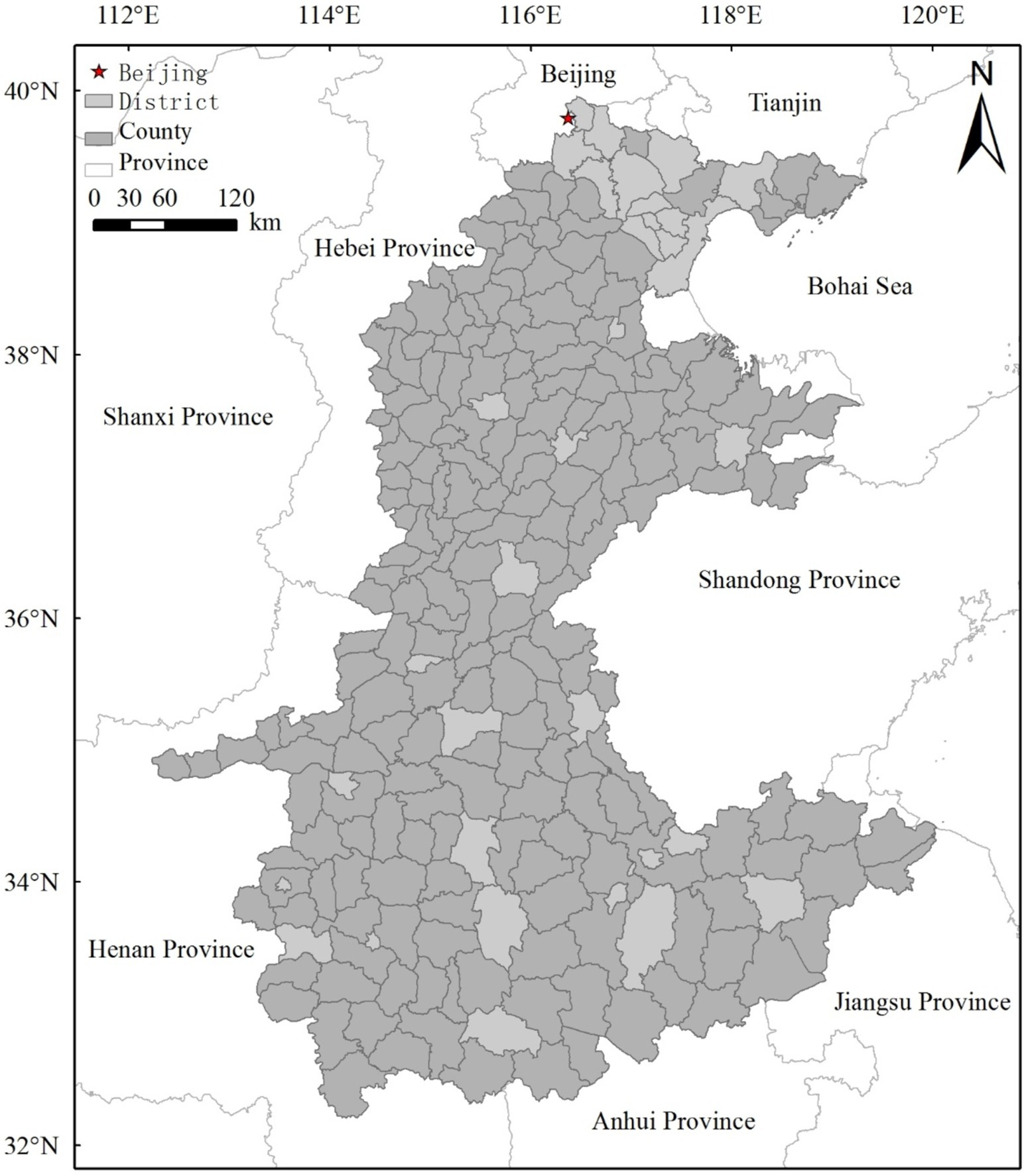
The North China Plain is located in the east of China, roughly between 32°and 40°N and 114°and 121E (Figure 1). It spans seven provinces and cities, including Beijing, Tianjin, Hebei, Shandong, Shanxi, Henan, Anhui, and Jiangsu, covering an area of 0.23 million km². It is a flat terrain, with the highest elevation below 50 m. It lies in the warm temperate zone, with changing four seasons. The southern part is in the subtropical transition zone. The mean annual temperature ranges between 8°C and 15°C, and annual rainfall varies between 500 mm and 900 mm. Both temperature and rainfall increase on going from north to south. Due to its favorable terrain conditions and abundant natural resources, this region has always been the political, economic, and cultural center of China. Beijing, the capital of China, is located at the north of the North China Plain. Despite rapid urbanization since reforms, many rural areas remain widely distributed. The North China Plain has the highest density of rural settlements and the largest percentage of rural settlements in China (Tian et al., 2007). Furthermore, the rural settlement of the North China Plain accounts for 31.44% of the national rural settlements (Tian et al., 2007).

Figure 1

Figure 1. Location of the study area.

Data source and pre-processing

Rural settlement data

The data on the rural settlements were interpreted using Landsat 8 images with 30 m resolution, which were collected in 2020 from the United States Geological Survey (USGS),¹ considering the cloud cover and vegetation phenology.

Influencing factor data

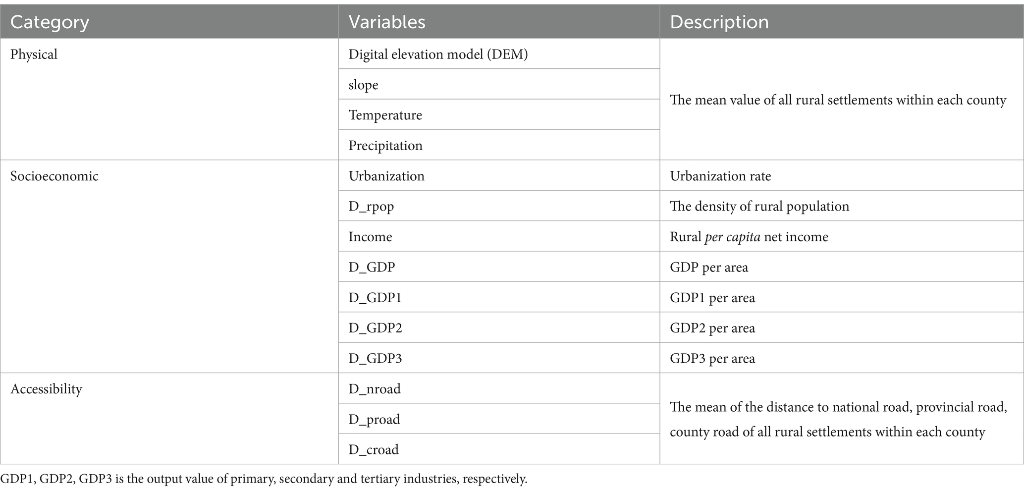
Given the data accessibility, comparable to previous studies, and the actual situation of the North China Plain, 14 potential factors influencing the spatial distribution of rural settlement at the county level and covering physical, socioeconomic, and accessibility were selected (Table 1).

Table 1

Table 1. The potential influencing factors of rural settlement distribution.

The selected potential physical factors include elevation, slope, temperature, precipitation. The DEM data set with a resolution of 90 m was obtained from the resource and environmental science data platform, Chinese Academy of Sciences.² The slope image was generated from the DEM data set. The meteorological data were sourced from the China meteorological data network.³ We obtained the related raster surface of the North China Plain by using Inverse distance weighting (IDW) interpolation. To get the mean value of potential influences at county level, we first extracted the values corresponding to each rural settlement site from related raster surfaces, and then the mean value at the county level was calculated using the points that fall inside each county.

The socioeconomic data were collected from China Statistical Yearbook for Regional Economy, China County Statistical Yearbook, China City Statistical Yearbook, Hebei Economic Yearbook, Shandong Statistical Yearbook, Henan Statistical Yearbook, Anhui Statistical Yearbook, and Jiangsu Statistical Yearbook, and it included total population, rural population, rural per capita net income, the output value of primary (GDP1), secondary (GDP2), and tertiary (GDP3) industries for each county in 2020. Furthermore, the urbanization rate, the density of rural population, rural per capita net income, GDP per area, GDP1 per area, GDP2 per area, and GDP3 per area for each county were calculated. Finally, they were converted into spatial data by linking them to the corresponding county administrative divisions in ArcGIS 10.5.

The accessibility data represent the mean value of the distance to the national road, provincial road, and county road of all rural settlements within each county. The road map was obtained from the China electric map. Additionally, the administrative zoning map of China at the county level was provided by the Data Sharing Infrastructure of Earth System Science.⁴

Methods

The interpretation of rural settlement

The process of the interpretation of rural settlements mainly include three steps: remote sensing image cropping, the interpretation of image, and the revision of the preliminary interpretation results. First, the study area was divided into different parts with appropriate sizes according to the available part of the corresponding image. The availability was determined based on cloud-free conditions and the obvious differences between rural settlements and other classes. Then, the available part of the corresponding image was extracted using ENVI 5.1 for later use.

During the second step, the process of interpretation based on eCognition developer 8.9 mainly includes two parts: segmentation and classification. After several repeated attempts, the scale parameter of multiresolution segmentation is set to 125–130. The nearest neighbor algorithm is used to take the mean value of each sample as the feature space of the corresponding class. Finally, when the function of classification is run, we obtain the preliminary results of interpretation.

The third step is the artificial visual modification, which is the most time-consuming stage. The fundamental principle in this modification is revising the preliminary results of interpretation according to the corresponding image. It mainly consists of three aspects. First is the adding the rural settlement that was not identified in the preliminary results of interpretation but that which exists on the image. The second step involves deleting the rural settlements that were provided in the preliminary results of interpretation but that which do not exist on the image. Third, the scope of some settlements may be not be accurate, which need to be further reshaped according to the image.

Spatial regression

In this study, we investigated the spatial relationship between the amount and area of rural settlements and related factors at the county level. Considering the types of variables, both multiple liner regression and Poisson regression analyses were employed. Furthermore, they were carried out from both the global and local perspectives.

Before performing the regression analysis, all the independent variables were standardized (Dong et al., 2016). Pearson’s correlation coefficient was employed to confirm that the potential linear relationships existed between the dependent variable and corresponding independent variables. Stepwise regression was utilized to select the most important predictors at a significance level of $\alpha =0.05$ and specify a useful regression model (Kauhl et al., 2015; Zhen et al., 2013).

Global model

Multiple linear regression

The total area of rural settlements is a continuous variable. Then, the multiple linear regression technique is applied, which can be described as follows Equation 1:

$\begin{array}{ll}\mathrm{y}={\beta }_0+{\displaystyle \sum _{i=o}^n}{\beta }_n{x}_n+\epsilon & (1)\end{array}$

Where y is the estimated value of the dependent variable. ${\beta }_0$ represents the intercept, and ${\beta }_n$ is the regression coefficient of the independent variable $x_n$. $\epsilon$ denotes the random error term.

Poisson regression

The number of rural settlements is a countable variable and Poisson regression Equation 2 may be the appropriate model for determining it (Wei et al., 2024):

$\begin{array}{ll}\ln \left(y\right)={\beta }_0+{\displaystyle \sum _{i=o}^k}{\beta }_k{x}_k& (2)\end{array}$

Where ln(y) is the natural log of the number of rural settlements for each county. ${\beta }_0$ is a constant, and ${\beta }_k$ is the regression coefficient of the independent variable $x_k$.

However, the regression coefficient of independent variables is assumed to be constant across space in these two global models. Furthermore, the spatial effects (spatial autocorrelation and heterogeneity) of the dependent variables may make the results of regression models less reliable (Shafizadeh-Moghadam and Helbich, 2015; Zhen et al., 2013). Therefore, the corresponding local model, geographically weighted regression and geographically weighted Poisson regression, can serve as a supplement to the regression and may be more efficient.

Local model

Geographically weighted regression

Geographically weighted regression is used to model continuous responses such as the area of rural settlements for each county in this study. GWR can be expressed as follows Equation 3 (Zhou and Lu, 2023):

$\begin{array}{ll}{y}_i={\beta }_0\left(u_i,v_i\right)+{\displaystyle \sum _{j=1}^k}{\beta }_j\left(u_i,v_i\right)x_{ij}+{\epsilon }_i& (3)\end{array}$

Where $\left(u_i,v_i\right)$ denotes the coordinate location of the ith point; ${\beta }_0\left(u_i,v_i\right)$ is the intercept at location i; ${\beta }_j\left(u_i,v_i\right)$ is the local estimated coefficient for $x_{ij}$; and ${\epsilon }_i$ is the random error term.

Geographically weighted Poisson regression

Geographically weighted Poisson regression is used to locally predict the count variables such as the number of rural settlements for each county in this study. GWPR can be written as Equation 4 (Zhen et al., 2013):

$\begin{array}{ll}\ln \left(y_i\right)={\beta }_0\left(u_i,v_i\right)+{\displaystyle \sum _{j=1}^k}{\beta }_j\left(u_i,v_i\right)x_{ij}+{\epsilon }_i& (4)\end{array}$

Where ${\beta }_j\left(u_i,v_i\right)$ is the regression coefficient for predictor $x_{ij}$ at location $\left(u_i,v_i\right)$.

The local model extends the corresponding global model by generating a local regression equation with a group of coefficients for each observation. The local coefficient is calculated based on the continuous function for the location $\left(u_i,v_i\right)$. The closer the specific location, the higher the weight will be and vice versa.

The fixed Gaussian and adaptive bi-square kernel functions are commonly used to determine how many nearest-neighbor observations are taken into consideration per local regression. The fixed kernel function applies an optimal spatial kernel (bandwidth) over the space, while the adaptive kernel function ensures a certain number of nearest neighbors as local samples (Fotheringham et al., 2003; Luo and Wei, 2009). The adaptive bandwidth is appealing especially when the distribution of the data point is heterogeneous (Fotheringham et al., 2003; Shafizadeh-Moghadam and Helbich, 2015). Thus, the adaptive bi-square kernel function Equation 5 is applied in this study as follows:

$w_{ij}=\{\begin{array}{c}{\left(1-d_{ij}^2/{\theta }_{i\left(k\right)}\right)}^2{d}_{ij}<{\theta }_{i\left(k\right)}\\ 0d_{ij}>{\theta }_{i\left(k\right)}\end{array}\text{ (5)}$

Where i is the regression point index; j is the locational index; $w_{ij}$ is the weight value of observation at location j for estimating the coefficient at location i. $d_{ij}$ is the Euclidean distance between i and j; $\mathrm{\theta }$ is a fixed bandwidth size defined by a distance metric measure; ${\theta }_{i\left(k\right)}$ is an adaptive bandwidth size defined as the k th nearest neighbor distance.

The selection of optimal bandwidth is based on the Akaike’s information criterion (AIC). Moreover, it can also be used to select the optimal model. A smaller AIC value is preferred.

Results

Spatial distribution of rural settlements

The total number and density of rural settlements in the study area is 144,941 and 0.51/km², respectively, covering an area of 26,214.23 km², accounting for 10.30% of the North China Plain. The spatial distribution of rural settlements shows a clear spatial agglomeration feature, especially the density (Figure 2). The density of rural settlements within each county ranges from 0/km² to 1.11/km², decreasing from the south to the north. Specifically, it is shaped like a ring with Henan–Anhui border as the high-value center in the south of the North China Plain; it increases from west to east with its value ranging from 0.29/km² to 0.81/km² in the middle part; its low-value center looks like a horizontal “Y” around the Circum–Bohai Sea region. Similarly, the maximum percentage of rural settlements within a county is 17.81% found in the south of the North China Plain, and the minimum is located in the north of the study area. In addition, the rural settlements with <8.92% of the country are concentrated in the northeast of the North China Plain.

Figure 2

Figure 2. Spatial distribution of the density and percentage of rural settlement at the county level.

Results of Pearson’s correlation analysis

The Pearson’s correlation coefficients between the density of rural settlements and 15 standardized independent variables show that all variables except DEM and GDP1 have a significant correlation (Table 2). Only slope and the distance to provincial road show a significant correlation at the 0.05 level, while others are significant at the 0.01 level. The distance to county road, GDP, GDP2, GDP3, urbanization, and income have a negative correlation with the dependent variable, while others show a positive correlation.

Table 2

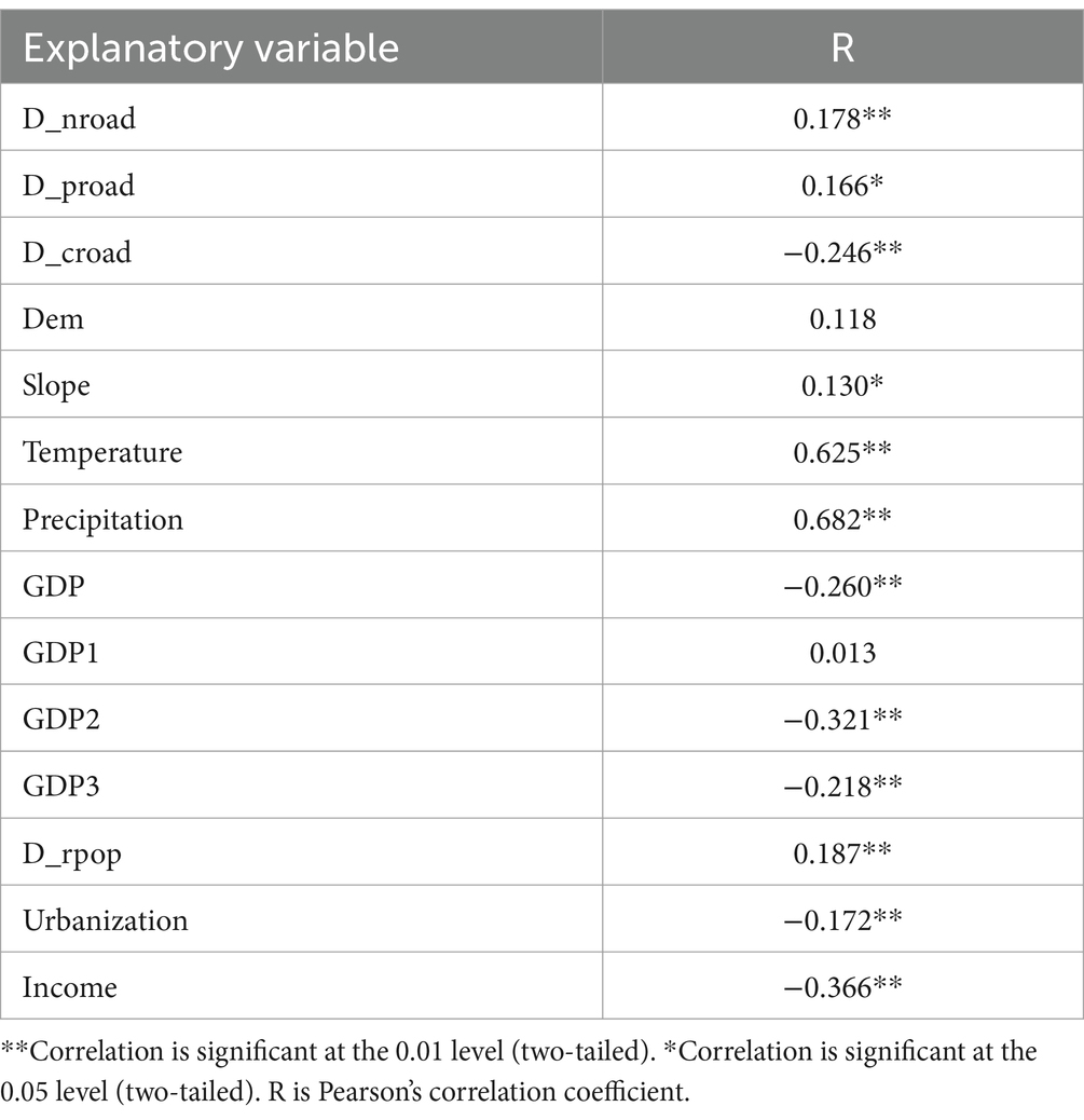
Table 2. Pearson’s correlation coefficients between the density of rural settlement and explanatory variables.

Pearson’s correlation coefficients between the number of rural settlements within each county and 15 potential independent variables are shown in Table 3. Similar results were found, and all independent variables except the distance to national road and distance to provincial road have a significant correlation with the dependent variable. In addition to the distance to county road and slope at the level of significance of 0.05, other factors were significant at the level of 0.01. In addition, the distance to county road, slope, GDP, GDP2, GDP3, urbanization, and income show a negative effect.

Table 3

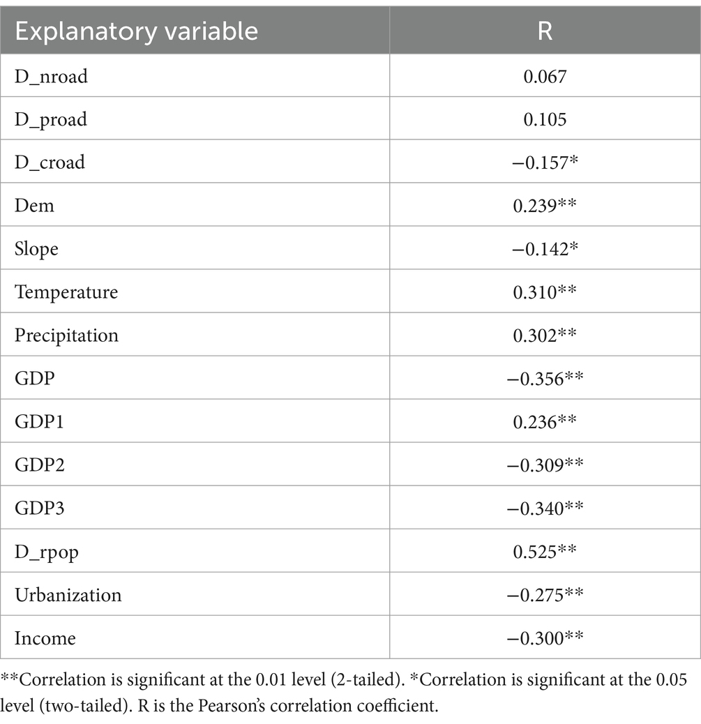
Table 3. Pearson’s correlation coefficients between the percentage of rural settlement and explanatory variables.

Based on the results of Pearson’s correlation, factors that pass the significance test are the potential factors for the area and number of rural settlements and will be used in the stepwise regression for exploratory analysis.

Results of the global models

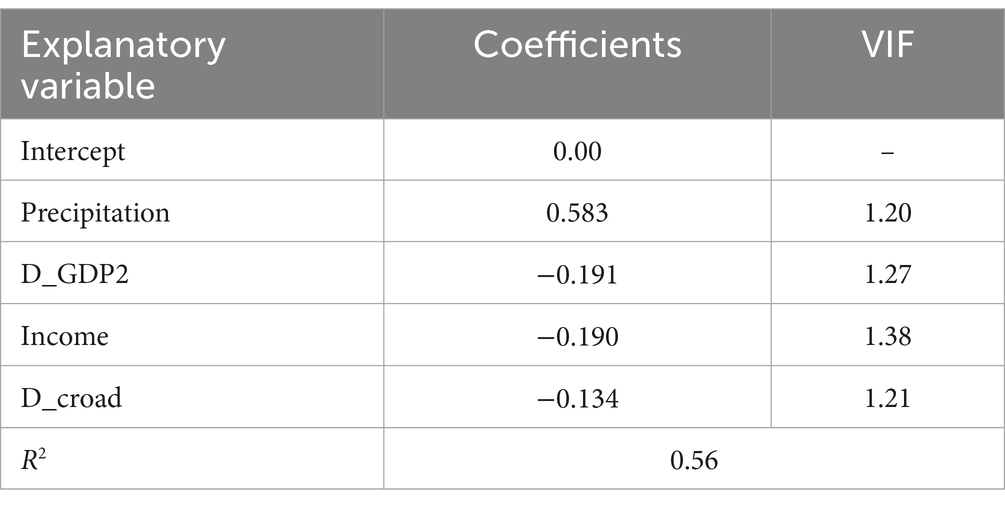
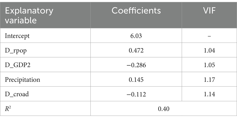
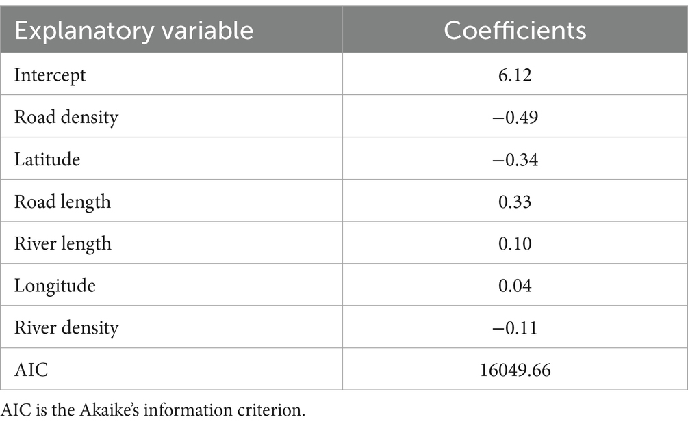
Multiple linear regression analysis was performed using a stepwise method, and the results are shown in Tables 4, 5. Only precipitation, GDP2 per area, income, and distance to county road enter the regression model for the density of rural settlements. In the regression equation, only precipitation has a positive coefficient, while others show a negative sign. In the final regression model for the number of rural settlements, the density of rural population, GDP2 per area, precipitation, and distance to county road act as the independent variables. Negative signs are observed for GDP2 per area and distance to county road. Furthermore, the Variance inflation factor of the two models all below 10 indicates that multicollinearity does not pose a problem. The R² value of multiple linear regression for the density and number of rural settlements is 0.56 and 0.40, respectively, indicating that the models perform well.

Table 4

Table 4. Results of global multiple linear regression for the density of rural settlements.

Table 5

Table 5. Results of global multiple linear regression for the percentage of rural settlements.

Results of local models

The local models were performed using the same data set with the corresponding final global models. The optimal bandwidth is 22 and 18 for GWR and GWPR, respectively. The GWPR model calculates an additional global Poisson regression model, which can be compared to the results of the global multiple linear regression model and the local Poisson regression model (Kauhl et al., 2015). The results of the Poisson regression model are similar to those of the corresponding multiple linear regression model (Tables 5, 6).

Table 6

Table 6. Results of global Poisson regression for the number of rural settlements.

Descriptive statistics of coefficients

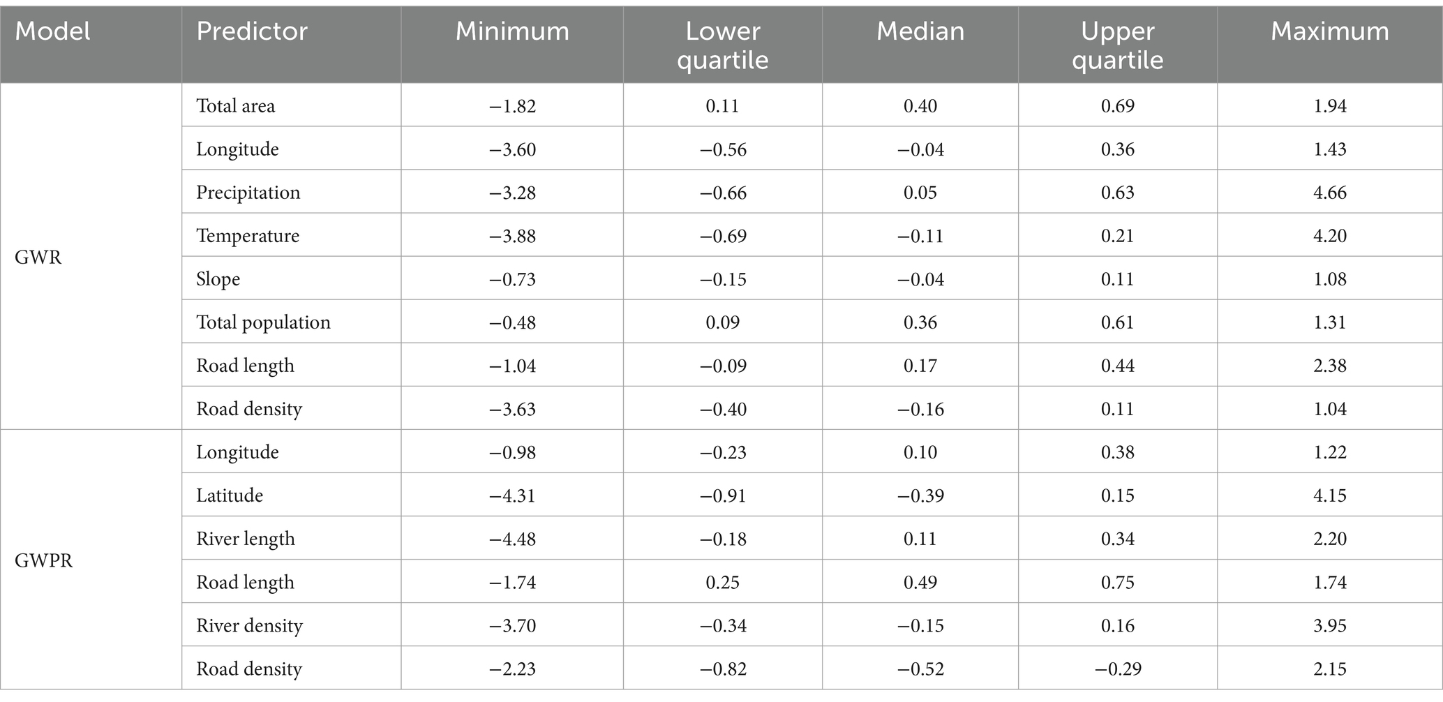
In contrast to the constant coefficients in global model, both the magnitude and sign of the coefficients in the local model show a spatial variation (Table 7). In the GWR model, only the minimum coefficient of total population and total area is negative, but other statistics for coefficients of these predictors are positive. Most coefficients of precipitation and road length are positive, as evident from the positive median, upper quartile, and maximum of coefficients. The upper quartile and maximum of longitude, temperature, slope, and road density are positive; however, most coefficients of these predictors are negative according to the negative median, lower quartile, and minimum.

Table 7

Table 7. Descriptive statistics of coefficients in the local models.

In the GWPR model, only the minimum coefficient of road length is negative, while other statistics are positive. On the contrary, the maximum coefficient of road density is the only positive variable, while other statistics are negative. The minimum and lower quartile coefficients of longitude and river length are <0, but the median, upper quartile, and maximum coefficients are positive. The minimum, lower quartile, and median of the latitude and river density are negative, while the upper quartile and maximum is positive.

Comparing the coefficients of the local and global models (Tables 4–7), it can be found that the coefficients of the global model fall into the range of coefficients of the local model. Furthermore, it is worth noting that the sign of the median of the coefficients in local models is the same as the sign of corresponding coefficients in the global models. In other words, despite the coefficients of the local model showing both negative and positive effects simultaneously, they did follow a similar tendency of signs in the corresponding global models.

Spatial distribution of coefficients

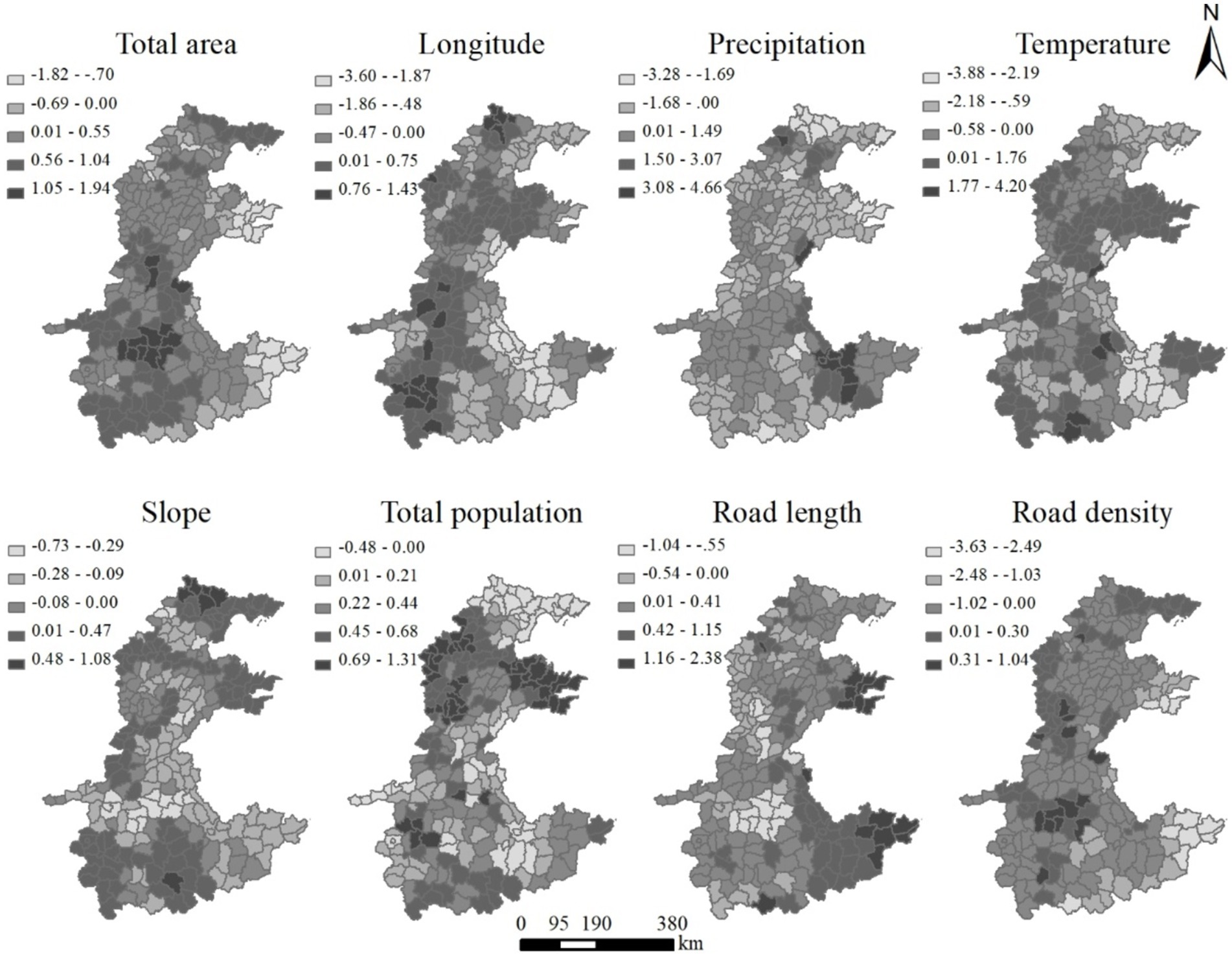
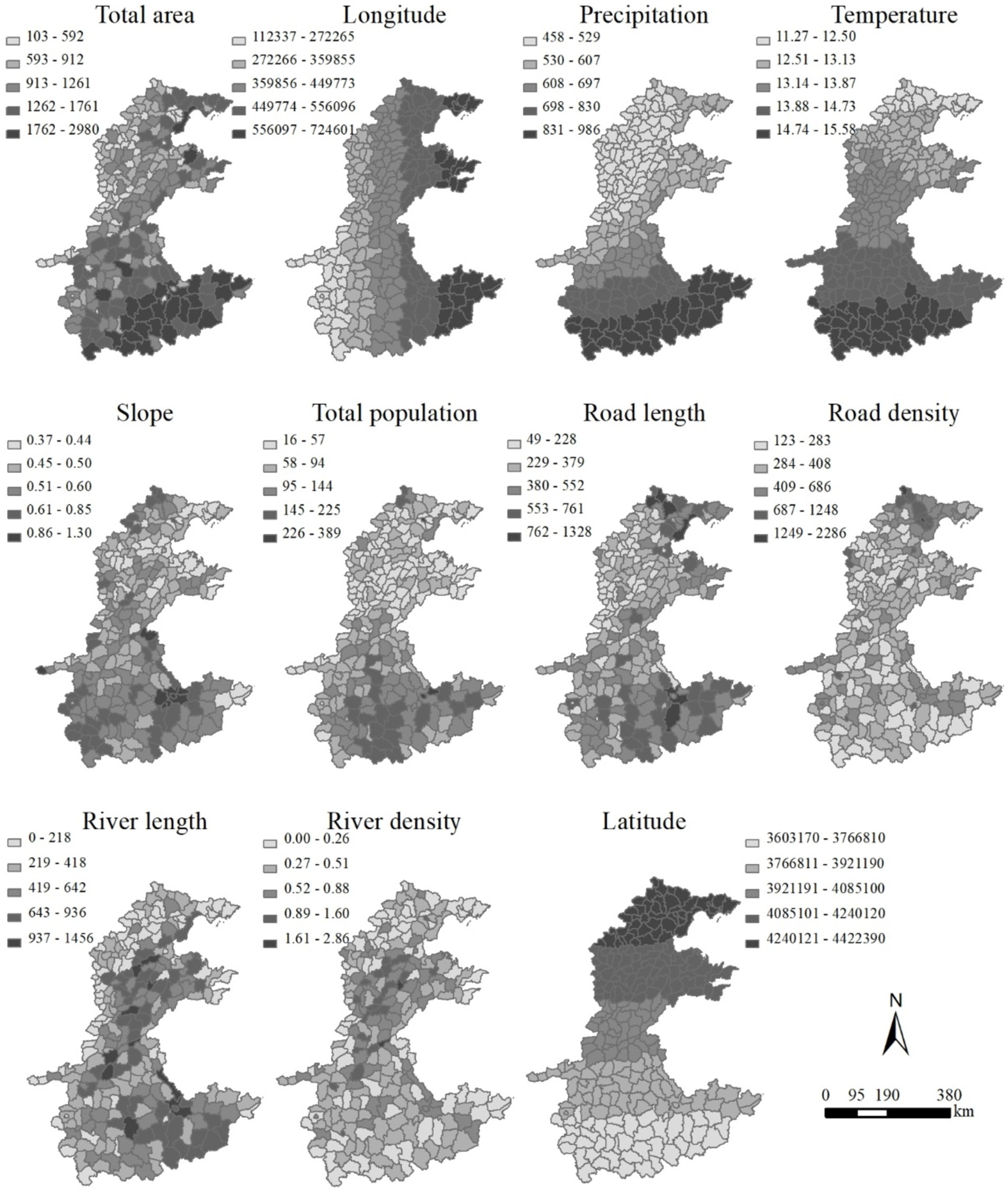
The spatial distribution of coefficients of the GWR model is shown in Figure 3. It is detected that all coefficients have an obvious pattern of spatial heterogeneity. The coefficients of the total area ranges from −1.82 to 1.94. However, in large parts of the North China Plain, the total area shows an expected positive impact. In addition, the coefficients are relatively larger in the southern part than in the northern part, which matches with the spatial distribution of the total area (total area in Figures 3, 4). Both positive and negative effects are found in longitude. In the west, especially the southwest, it was dominated by the positive coefficients while the negative values are mainly concentrated in the east part, especially the southeast, which is similar to the distribution of longitude (Longitude of Figures 3, 4). Similarly, precipitation also indicates both positive and negative coefficients and their number is almost the same. In addition, the positive coefficients are mainly located in the south where the precipitation is relatively higher (Precipitation in Figures 3, 4). For temperature and slope, the negative and positive coefficients are crossed and distributed in the study area (Figure 3, temperature and slope). The coefficients of slope are relatively small compared to those of other influences, indicating it has a weaker impact on the distribution of the rural settlements. For total population, the expected positive value is widely spread in the study area with relatively large coefficients located in the north and middle part of the North China Plain, while the negative effect was only found in the north and some areas around the municipal district (Figure 3, Total population). It should be noted that the coefficients of total population range from −0.48 to 1.31, which is relatively small. The positive coefficients of road length also take a large proportion of the study area with the value decreasing from east to west, while the negative coefficients are mainly concentrated in the northwest part, where the road length is relatively small (road length in Figures 3, 4). On the contrary, the road density indicates a negative effect in most parts, while the positive values only occurred in the west and northeast (Figure 3, road density).

Figure 3

Figure 3. Coefficients of explanatory variables in GWR.

Figure 4

Figure 4. Distribution of the predictors.

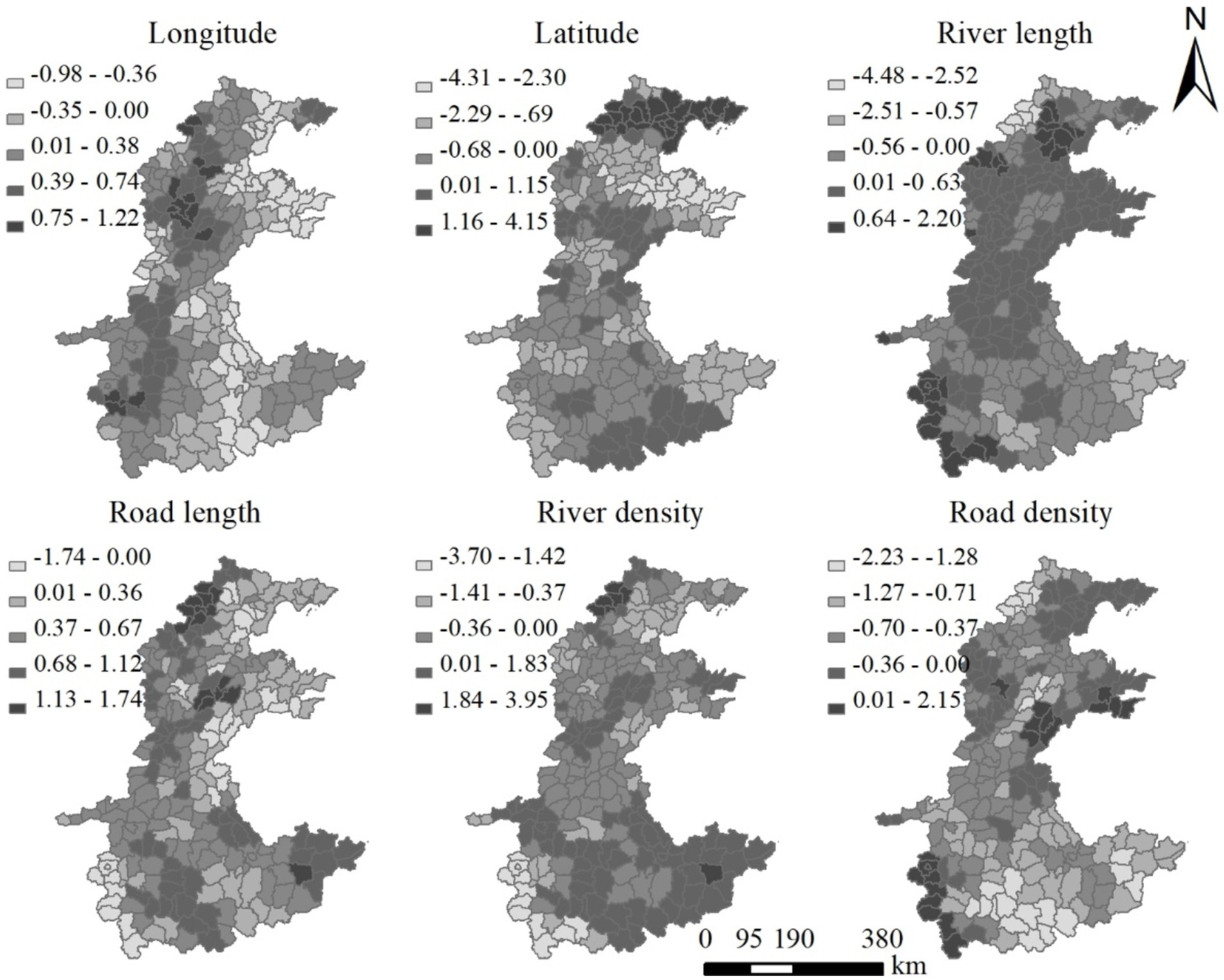
Figure 5 presents the coefficient surfaces of the six factors used in the GWPR model. Similar to the results of GWR, the coefficients also vary across the study area. All the six factors show both negative and positive effects on the number of rural settlements. The coefficients of longitude show a difference between the west and east, which matches the distribution of longitude. The negative coefficients of longitude are located in the east of the North China Plain, while the west mainly has a positive value (Longitude in Figures 4, 5). In most parts, the coefficients of latitude is <0, while the positive value only occurs in three belts in the direction of west–east in the north, middle, and south of the study area (Figure 5, Latitude). The negative coefficients of the river length is mainly located in the southeast and northwest, while most parts show a positive value (Figure 5, River length). In the most parts of the North China Plain (201 counties), road length has a positive coefficient. In contrast, the coefficients of road density are negative in large parts of the study area. It worth noting that the area with a negative coefficient of road length and the area showing a positive value of road density have some spatial intersection (Figure 5, Road length and Road density). The minority of coefficients of river density is positive and mainly distributed in the south of the study area (Figure 5, River density).

Figure 5

Figure 5. Coefficients of explanatory variables in GWPR.

Comparisons between global and local models

Model performance

AIC is the frequently used criterion to evaluate the performance of models, and a lower AIC value is preferred (Fotheringham et al., 2001). The AIC values of global and local models for the number of rural settlements are 16049.66 and 1392.00, respectively. The corresponding results for the area of rural settlement are 235.04 and 3.81, respectively. Compared to the global models, the values of AIC from local models are much lower. All these results suggest that local models are superior in explaining the relationships between the area/number of rural settlements and related factors.

Spatial autocorrelations in model residuals

The global Moran’s I of model residual is calculated to explore the spatial autocorrelation of the residual. The Moran’s I of global Poisson and multiple linear regression models is 0.12 and 0.08, respectively, with the corresponding p-value of 0.09 and 0.24. It indicates that there is no significant spatial autocorrelation in the residual of the global model. By contrast, the results of the local model, geographically weighted Poisson regression and geographically weighted regression, show a smaller Moran’s I (−0.01 and 0.00) and a larger p-value (0.94 and 0.96), suggesting there is no problem of spatial autocorrelation in the residuals of the local model.

Discussion

Spatial pattern of rural settlements

The distribution of rural settlements in the North China Plain show obvious spatial characteristics, with both the number and area of the county decreasing from north to south and from east to west. However, this finding is inconsistent with the result of Tan and Li (2013) who reported that rural settlements were evenly distributed in rural areas in both 1970s and 2007. This can be because our study area is much larger. Our study area, the North China Plain, includes 201 counties, while Daxing district, which is only equal to one county in area, was the study area in Tian et al. (2012) study. Moreover, the results of Tian et al. (2012) support this viewpoint.

Accordingly, it can be concluded that rural settlements are evenly distributed in the local distribution due to the landform (mainly flat plains), historical tradition, and the agricultural land system (Ma et al., 2022; Tan and Li, 2013), while it shows an obvious spatial difference on a large scale owing to the natural conditions, customs, and house styles (Song and Li, 2020).

Influence of the spatial distribution of rural settlements

The results of Pearson’s correlation show that only elevation, GDP, and rural population have no significant relationship with the area and number of rural settlements. Besides, the rural per capita net income shows a negative correlation. The irrelevant correlation between elevation and the area of rural settlement is understandable given that the North China Plain is a flat terrain with no great difference in elevation. GDP also having no significant relationship is also comprehensible, because GDP may have a main impact only on urban expansion (Chen et al., 2019; Seto et al., 2011).

However, it is very interesting that rural population has no significant relationship with the distribution of rural settlements and that rural per capita net income has a negative correlation with the distribution of rural settlements, which is in disagreement with previous studies (Long et al., 2009; Yang et al., 2019; Yin et al., 2023). One reason may be that the rural settlement area was decoupled from the rural population (Dong et al., 2021; Zhu et al., 2020). Tian et al. (2014) also found that Beijing experienced a 33.6% increase in the rural settlement land and a 34.8% decline in its rural population. Another possible explanation is that the farmer’s income is no longer the limitation for building rural houses. The farmer’s income of China is very low and has been a limitation for building new houses for a long time in the past. And at that stage, they used to build a more comfortable or spacious house when they can afford it (Qu et al., 2021). However, China has undergone rapid development and entered a new growth stage, which has improved the farmer’s income significantly and no longer limits the development of the rural house. On the other hand, the majority of the next generation of farmers received good education in university or work in urban areas. And some of them would not return to rural areas. Thus, instead of building a new house in the rural area, they would save money for buying a house in the urban area. Last, but not the least, instead of rural residence land, other construction lands such as the industrial land has been the dominant component of rural settlement expansion (Kuang et al., 2016).

Interpretation of the spatially varying relationships

From the perspective of the magnitude of coefficients, the coefficients of the global model are constant within the range of the coefficients of the local model. It indicates that the global model only reflects the overall condition of the study area, while the local model provides more details for each location. It is in accordance with previous studies (Gao and Li, 2011; Guanglong et al., 2017; Li et al., 2013).

From the perspective of the sign of coefficients, different from the invariable sign of coefficient in the global model, both negative and positive signs are included in the local model simultaneously in this study. In addition, some signs of coefficients are counterintuitive or unexpected. However, it is not uncommon in GWR or GWPR models and are consistent with previous studies (Chow et al., 2006; Hadayeghi et al., 2010; Luo and Wei, 2009; Wheeler and Calder, 2007; Xu and Huang, 2015; Zhen et al., 2013). Despite the unexpected results, they may make sense when considering the physical truth of the study area in some case (Zhen et al., 2013), which is also the case for this study. For example, although it is expected that the total population has a positive impact on the distribution of rural settlements, total population with negative signs are also identified in the north of the study area and some areas around the municipal district. It was a bit of surprise, but it was because most of these counties with negative signs are close to the municipal district or of relatively high level of development, where the level of urbanization is relatively high and the development of rural settlements is under good control and management.

However, still several other possible explanations for this problem should be considered. First, the multicollinearity among some independent variables or the multicollinearity in local coefficients may be one possible reason. Although there is no problem with multicollinearity among the independent variables in the global model as indicated by their value of VIF < 10 in this study, there still may be multicollinearity among some independent variables in the local model (Hadayeghi et al., 2010; Xu and Huang, 2015). Besides, correlated local coefficients also could be a problem (Shariat-Mohaymany et al., 2015; Wheeler and Tiefelsdorf, 2005; Xu and Huang, 2015). The second possible reason is the significance of variables. Some variables may be less significant or even insignificant at all at some locations (Hadayeghi et al., 2010; Shariat-Mohaymany et al., 2015; Xu and Huang, 2015). Moreover, the missing or mis-specified explanatory variables in the model may also make some contribution to the unexpected signs (Hadayeghi et al., 2010; Shariat-Mohaymany et al., 2015). Finally, the bandwidth and the type of kernel function also have some influence on the range of the coefficients (Foody, 2003; Guanglong et al., 2017; Guo et al., 2008).

Consequently, the interpretation of the results of the local model should be done with caution and it is reasonable according to the reality of the study area, especially when counterintuitive signs are detected.

Advantages of the local model over the global model

In accordance with previous studies, our results also show that the local model, GWR, and GWPR, outperform the global model as evident by the lower AIC value (Guanglong et al., 2017; Luo and Wei, 2009; Zhen et al., 2013). Moreover, it does reduce the spatial autocorrelation in the model residual. However, we found that the local model helped reduce the spatial autocorrelation in residual even though there is no significant spatial autocorrelation problem in the global model. This result is a little different from previous studies (Gao and Li, 2011; Guo et al., 2008; Zhang et al., 2005; Zhen et al., 2013), which reported that the GWR model can reduce the spatial autocorrelations in residuals, especially while the significant spatial autocorrelation is found in the global model. Furthermore, our finding is inversed with Tu and Xia (2008) who found that the application of GWR may increase spatial autocorrelation if an ordinary least square (OLS) model does not have this problem.

Based on the shortcomings of the global model and the advantages of the local model, this article first reveals the driving factors of the spatial distribution of rural settlements from the global perspective, and then uncovers the spatial heterogeneity of the magnitude and direction of the driving factors from the local perspective. This is helpful to formulate different control measures for rural settlements according to the local conditions.

In addition, according to the basic principle of promoting rural revitalization by classification, the spatial heterogeneity of factors affecting the spatial distribution and evolution of rural settlements combined with the actual needs of China’s rural revitalization can be taken into account, and differentiated rural revitalization promotion strategies can be formulated by classification.

Conclusion

Scientifically revealing the spatially varying relationships between the distribution of rural settlements and related factors is fundamental for planning and management. The North China Plain is the main grain-producing region and a densely populated area in China. The contradiction between cultivated land protection and settlement expansion is prominent and severe. Thus, in this study, we investigated the spatial relationship between the distribution of rural settlement in the North China Plain and the related influences using geographically weighted regression.

The results show that the distribution of rural settlement in the North China Plain show an obvious spatial pattern, with both the number and the area of rural settlements at the county level increasing from north to south and from west to east. The results of the traditional regression model suggest that total area, total population, road density, precipitation, road length, slope, longitude and temperature are the significant factors influencing the total area, while those influencing the total number of rural settlements is longitude, latitude, road length, road density, river length, and river density. In addition, the coefficients of these influences are constant in the global model. However, both the magnitude and the sign of the corresponding parameters in the local model show a spatial variation. More interesting is that the value of the coefficients in global model fall into the range of the coefficients in the local model, and most coefficients in the local model share the same sign with those in the global model. This indicates that there is a significant spatial heterogeneity in the size and direction of the influencing factors. Therefore, the control measures of rural settlements with regional differences should be formulated according to local conditions.

Our results also reveal that the local model outperforms the global model with the same explanatory variables, as indicated by the smaller AIC value. Furthermore, the local model does help to reduce the spatial autocorrelation in model residual even when it is insignificant in the global model.

Although the local model has many advantages over the global model and can more efficiently reveal the spatially varying relationship, our results also highlight the importance of the cautious and scientific interpretation of the variations, especially when the unexpected results are obtained.

Data availability statement

The original contributions presented in the study are included in the article/supplementary material, further inquiries can be directed to the corresponding author.

Author contributions

CY: Writing – original draft, Writing – review & editing. GD: Conceptualization, Funding acquisition, Supervision, Writing – review & editing. ZL: Conceptualization, Formal analysis, Supervision, Writing – review & editing.

Funding

The author(s) declare that financial support was received for the research, authorship, and/or publication of this article. This study was supported by Humanities and Social Science Foundation of the Ministry of Education (Grant no. 23YJCZH038), Shandong Province social science planning research project (Grant no. 24CGLJ32), Natural Science Foundation of Shandong Province (Grant no. ZR2023MD061), and National Natural Science Foundation of China (Grant no. 41801173).

Conflict of interest

The authors declare that the research was conducted in the absence of any commercial or financial relationships that could be construed as a potential conflict of interest.

Generative AI statement

The author(s) declare that no Generative AI was used in the creation of this manuscript.

Publisher’s note

All claims expressed in this article are solely those of the authors and do not necessarily represent those of their affiliated organizations, or those of the publisher, the editors and the reviewers. Any product that may be evaluated in this article, or claim that may be made by its manufacturer, is not guaranteed or endorsed by the publisher.

Footnotes

1. ^http://glovis.usgs.gov/

2. ^https://www.resdc.cn

3. ^http://data.cma.cn/

4. ^http://www.geodata.cn/main/

References

Bi, G. H., and Yang, Q. Y. (2023). The spatial production of rural settlements as rural homestays in the context of rural revitalization: evidence from a rural tourism experiment in a Chinese village. Land Use Policy 128:106600. doi: 10.1016/j.landusepol.2023.106600

Crossref Full Text | Google Scholar

Brunsdon, C., Fotheringham, A. S., and Charlton, M. (1996). Geographically weighted regression: a method for exploring spatial non-stationarity. Geogr. Anal. 28, 281–298. doi: 10.1111/j.1538-4632.1996.tb00936.x

Crossref Full Text | Google Scholar

Chen, M., Gong, Y., Lu, D., and Ye, C. (2019). Build a people-oriented urbanization: China’s new-type urbanization dream and Anhui model. Land Use Pol. 80, 1–9. doi: 10.1016/j.landusepol.2018.09.031

Crossref Full Text | Google Scholar

Chen, S., Mehmood, M. S., Liu, S. C., and Gao, Y. M. (2022). Spatial pattern and influencing factors of rural settlements in Qinba Mountains, Shaanxi Province, China. Sustainability 14:95. doi: 10.3390/su141610095

Crossref Full Text | Google Scholar

Chen, S., Wang, X. Y., Qiang, Y., and Lin, Q. (2024). Spatial-temporal evolution and land use transition of rural settlements in mountainous counties. Environ. Sci. Eur. 36:868. doi: 10.1186/s12302-024-00868-y

Crossref Full Text | Google Scholar

Chen, M., and Ye, C. (2014). Differences in pattern and driving forces between urban and rural settlements in the coastal region of Ningbo, China. Sustainability 6, 1848–1867. doi: 10.3390/su6041848

Crossref Full Text | Google Scholar

Chow, L.-F., Zhao, F., Liu, X., Li, M.-T., and Ubaka, I. (2006). Transit ridership model based on geographically weighted regression. Transp. Res. Rec. J. Board 1972, 105–114. doi: 10.1177/0361198106197200113

Crossref Full Text | Google Scholar

de la Fuente, J. L. M., Infante-Amate, J., and Travieso, E. (2024). Historical changes in Mediterranean rural settlements (southern Spain, 1787-2019). J. Rural. Stud. 106:103217. doi: 10.1016/j.jrurstud.2024.103217

Crossref Full Text | Google Scholar

Dong, G., Xu, E., and Zhang, H. (2016). Spatiotemporal variation of driving forces for settlement expansion in different types of counties. Sustain. For. 8:39. doi: 10.3390/su8010039

Crossref Full Text | Google Scholar

Dong, G., Zhang, W., Xu, X., and Jia, K. (2021). Multi-dimensional feature recognition and policy implications of rural human–land relationships in China. Land 10:1086. doi: 10.3390/land10101086

Crossref Full Text | Google Scholar

Foody, G. (2003). Geographical weighting as a further refinement to regression modelling: an example focused on the NDVI–rainfall relationship. Remote Sens. Environ. 88, 283–293. doi: 10.1016/j.rse.2003.08.004

Crossref Full Text | Google Scholar

Fotheringham, A. S., Brunsdon, C., and Charlton, M. (2003). Geographically weighted regression: The analysis of spatially varying relationships. New York, NY: John Wiley & Sons.

Google Scholar

Fotheringham, A. S., Charlton, M. E., and Brunsdon, C. (2001). Spatial variations in school performance: a local analysis using geographically weighted regression. Geogr. Environ. Model. 5, 43–66. doi: 10.1080/13615930120032617

Crossref Full Text | Google Scholar

Gao, J., and Li, S. (2011). Detecting spatially non-stationary and scale-dependent relationships between urban landscape fragmentation and related factors using geographically weighted regression. Appl. Geogr. 31, 292–302. doi: 10.1016/j.apgeog.2010.06.003

Crossref Full Text | Google Scholar

Gong, J. Z., Jian, Y. Q., Chen, W. L., Liu, Y. S., and Hu, Y. M. (2022). Transitions in rural settlements and implications for rural revitalization in Guangdong Province. J. Rural. Stud. 93, 359–366. doi: 10.1016/j.jrurstud.2019.10.037

Crossref Full Text | Google Scholar

Guanglong, D., Erqi, X., and Hongqi, Z. (2017). The analysis of spatiotemporal varying relationships between urban expansion and related factors using geographically weighted regression. Appl. Geograph. 8, 277–286.

Google Scholar

Guo, L., Ma, Z., and Zhang, L. (2008). Comparison of bandwidth selection in application of geographically weighted regression: a case study. Can. J. For. Res. 38, 2526–2534. doi: 10.1139/X08-091

Crossref Full Text | Google Scholar

Hadayeghi, A., Shalaby, A. S., and Persaud, B. N. (2010). Development of planning level transportation safety tools using geographically weighted Poisson regression. Accid. Anal. Prev. 42, 676–688. doi: 10.1016/j.aap.2009.10.016

PubMed Abstract | Crossref Full Text | Google Scholar

Huang, J., Huang, Y., Pontius, R. G., and Zhang, Z. (2015). Geographically weighted regression to measure spatial variations in correlations between water pollution versus land use in a coastal watershed. Ocean Coastal Manage. 103, 14–24. doi: 10.1016/j.ocecoaman.2014.10.007

Crossref Full Text | Google Scholar

Ivajnšič, D., Kaligarič, M., and Žiberna, I. (2014). Geographically weighted regression of the urban heat island of a small city. Appl. Geogr. 53, 341–353. doi: 10.1016/j.apgeog.2014.07.001

Crossref Full Text | Google Scholar

Jia, K. Y., Qiao, W. F., Chai, Y. B., Feng, T., Wang, Y. H., and Ge, D. Z. (2020). Spatial distribution characteristics of rural settlements under diversified rural production functions: a case of Taizhou, China. Habitat Int. 102:102201. doi: 10.1016/j.habitatint.2020.102201

Crossref Full Text | Google Scholar

Kauhl, B., Heil, J., Hoebe, C. J., Schweikart, J., Krafft, T., and Dukers-Muijrers, N. H. (2015). The spatial distribution of hepatitis C virus infections and associated determinants—an application of a geographically weighted Poisson regression for evidence-based screening interventions in hotspots. PLoS One 10, 1–19. doi: 10.1371/journal.pone.0135656

Crossref Full Text | Google Scholar

Kong, X. S., Liu, D. F., Tian, Y. S., and Liu, Y. L. (2021). Multi-objective spatial reconstruction of rural settlements considering intervillage social connections. J. Rural. Stud. 84, 254–264. doi: 10.1016/j.jrurstud.2019.02.028

Crossref Full Text | Google Scholar

Kuang, W., Liu, J., Dong, J., Chi, W., and Zhang, C. (2016). The rapid and massive urban and industrial land expansions in China between 1990 and 2010: a CLUD-based analysis of their trajectories, patterns, and drivers. Landsc. Urban Plan. 145, 21–33. doi: 10.1016/j.landurbplan.2015.10.001

Crossref Full Text | Google Scholar

Li, L., Li, X. J., Hai, B. B., Wang, X. F., and Xu, J. W. (2020). Evolution of rural settlement in an inland non-metropolitan region of China at a time of rapid urbanisation: the case of Gongyi. J. Rural. Stud. 79, 45–56. doi: 10.1016/j.jrurstud.2020.08.003

Crossref Full Text | Google Scholar

Li, T., Long, H., Liu, Y., and Tu, S. (2015). Multi-scale analysis of rural housing land transition under China’s rapid urbanization: the case of Bohai rim. Habitat Int. 48, 227–238. doi: 10.1016/j.habitatint.2015.04.002

Crossref Full Text | Google Scholar

Li, H. H., and Song, W. (2019). Expansion of rural settlements on high-quality arable land in Tongzhou District in Beijing, China. Sustainability 11:19. doi: 10.3390/su11195153

Crossref Full Text | Google Scholar

Li, J. F., and Song, W. (2023). Review of rural settlement research based on bibliometric analysis. Front. Environ. Sci. 10:1089438. doi: 10.3389/fenvs.2022.1089438

Crossref Full Text | Google Scholar

Li, K. M., Wang, M., Hou, W. B., Gao, F. Y., Xu, B. C., Zeng, J. J., et al. (2023). Spatial distribution and driving mechanisms of rural settlements in the Shiyang River basin, Western China. Sustainability 15:126. doi: 10.3390/su151612126

Crossref Full Text | Google Scholar

Li, Z., Wang, W., Liu, P., Bigham, J. M., and Ragland, D. R. (2013). Using geographically weighted Poisson regression for county-level crash modeling in California. Saf. Sci. 58, 89–97. doi: 10.1016/j.ssci.2013.04.005

Crossref Full Text | Google Scholar

Lin, F. F., Cheng, P., and Kong, X. S. (2023). Spatiotemporal interaction between rural settlements and cultivated land in karst mountainous area, China. Chin. Geographic. Sci. 33, 946–965. doi: 10.1007/s11769-023-1373-x

Crossref Full Text | Google Scholar

Long, H., Li, Y., Liu, Y., Woods, M., and Zou, J. (2012). Accelerated restructuring in rural China fueled by ‘increasing vs. decreasing balance’ land-use policy for dealing with hollowed villages. Land Use Pol. 29, 11–22. doi: 10.1016/j.landusepol.2011.04.003

Crossref Full Text | Google Scholar

Long, H., Liu, Y., Wu, X., and Dong, G. (2009). Spatio-temporal dynamic patterns of farmland and rural settlements in Su–Xi–Chang region: implications for building a new countryside in coastal China. Land Use Policy 26, 322–333. doi: 10.1016/j.landusepol.2008.04.001

Crossref Full Text | Google Scholar

Luo, J., and Wei, Y. D. (2009). Modeling spatial variations of urban growth patterns in Chinese cities: the case of Nanjing. Landsc. Urban Plan. 91, 51–64. doi: 10.1016/j.landurbplan.2008.11.010

Crossref Full Text | Google Scholar

Ma, W. Q., Jiang, G. H., Li, W. Q., Zhou, T., and Zhang, R. J. (2019). Multifunctionality assessment of the land use system in rural residential areas: confronting land use supply with rural sustainability demand. J. Environ. Manag. 231, 73–85. doi: 10.1016/j.jenvman.2018.09.053

PubMed Abstract | Crossref Full Text | Google Scholar

Ma, L. B., Li, J. Y., Wang, X., Zhang, W. B., Tao, T. M., and Zhong, Y. (2024). Evolution and simulation optimization of rural settlements in urban-rural integration areas from a multi-gradient perspective: a case study of the Lan-Bai urban agglomeration in China. Habitat Int. 153:103203. doi: 10.1016/j.habitatint.2024.103203

Crossref Full Text | Google Scholar

Ma, L. B., Liu, S. C., Tao, T. M., Gong, M., and Bai, J. (2022). Spatial reconstruction of rural settlements based on livability and population flow. Habitat Int. 126:102614. doi: 10.1016/j.habitatint.2022.102614

Crossref Full Text | Google Scholar

Martínez-Fernández, J., Chuvieco, E., and Koutsias, N. (2013). Modelling long-term fire occurrence factors in Spain by accounting for local variations with geographically weighted regression. Nat. Hazards Earth Syst. Sci. 13, 311–327. doi: 10.5194/nhess-13-311-2013

Crossref Full Text | Google Scholar

Qu, Y. B., Jiang, G. H., Ma, W. Q., and Li, Z. T. (2021). How does the rural settlement transition contribute to shaping sustainable rural development? Evidence from Shandong, China. J. Rural. Stud. 82, 279–293. doi: 10.1016/j.jrurstud.2021.01.027

Crossref Full Text | Google Scholar

Ran, D., Hu, Q. Y., and Zhang, Z. L. (2024). Spatial-temporal evolution, impact mechanisms, and reclamation potential of rural human settlements in China. Land 13:430. doi: 10.3390/land13040430

Crossref Full Text | Google Scholar

Rao, Y. F., Zou, Y. F., Yi, C. F., Luo, F., Song, Y., and Wu, P. Q. (2023). Optimization of rural settlements based on rural revitalization elements and rural residents’ social mobility: a case study of a township in western China. Habitat Int. 137:102851. doi: 10.1016/j.habitatint.2023.102851

Crossref Full Text | Google Scholar

Rodrigues, M., de la Riva, J., and Fotheringham, S. (2014). Modeling the spatial variation of the explanatory factors of human-caused wildfires in Spain using geographically weighted logistic regression. Appl. Geogr. 48, 52–63. doi: 10.1016/j.apgeog.2014.01.011

Crossref Full Text | Google Scholar

Seto, K. C., Fragkias, M., Güneralp, B., and Reilly, M. K. (2011). A meta-analysis of global urban land expansion. PLoS One 6, 1–9. doi: 10.1371/journal.pone.0023777

Crossref Full Text | Google Scholar

Shafizadeh-Moghadam, H., and Helbich, M. (2015). Spatiotemporal variability of urban growth factors: a global and local perspective on the megacity of Mumbai. Int. J. Appl. Earth Obs. Geoinf. 35, 187–198. doi: 10.1016/j.jag.2014.08.013

Crossref Full Text | Google Scholar

Shariat-Mohaymany, A., Shahri, M., Mirbagheri, B., and Matkan, A. A. (2015). Exploring spatial non-stationarity and varying relationships between crash data and related factors using geographically weighted Poisson regression. Trans. GIS 19, 321–337. doi: 10.1111/tgis.12107

Crossref Full Text | Google Scholar

Song, W., Jia, H., Huang, J., and Zhang, Y. (2014). A satellite-based geographically weighted regression model for regional PM 2.5 estimation over the Pearl River Delta region in China. Remote Sens. Environ. 154, 1–7. doi: 10.1016/j.rse.2014.08.008

Crossref Full Text | Google Scholar

Song, W., and Li, H. H. (2020). Spatial pattern evolution of rural settlements from 1961 to 2030 in Tongzhou District, China. Land Use Pol 99:105044. doi: 10.1016/j.landusepol.2020.105044

Crossref Full Text | Google Scholar

Su, S., Li, D., Xiao, R., and Zhang, Y. (2014). Spatially non-stationary response of ecosystem service value changes to urbanization in Shanghai, China. Ecol. Indic. 45, 332–339. doi: 10.1016/j.ecolind.2014.04.031

Crossref Full Text | Google Scholar

Su, S., Zhang, Q., Zhang, Z., Zhi, J., and Wu, J. (2011). Rural settlement expansion and paddy soil loss across an ex-urbanizing watershed in eastern coastal China during market transition. Reg. Environ. Chang. 11, 651–662. doi: 10.1007/s10113-010-0197-2

Crossref Full Text | Google Scholar

Tan, M., and Li, X. (2013). The changing settlements in rural areas under urban pressure in China: patterns, driving forces and policy implications. Landsc. Urban Plan. 120, 170–177. doi: 10.1016/j.landurbplan.2013.08.016

Crossref Full Text | Google Scholar

Tan, M., Li, X., Xie, H., and Lu, C. (2005). Urban land expansion and arable land loss in China—a case study of Beijing–Tianjin–Hebei region. Land Use Policy 22, 187–196. doi: 10.1016/j.landusepol.2004.03.003

Crossref Full Text | Google Scholar

Tan, Y. X., Xiang, M. S., Lu, H. X., Duan, L. S., Yang, J., Meng, J. K., et al. (2023). Spatial difference studies and driving force analysis of rural settlements in the Northwest Sichuan plateau. Sustain. For. 15:7074. doi: 10.3390/su15097074

Crossref Full Text | Google Scholar

Tian, G., Qiao, Z., and Gao, X. (2014). Rural settlement land dynamic modes and policy implications in Beijing metropolitan region, China. Habitat Int. 44, 237–246. doi: 10.1016/j.habitatint.2014.06.010

Crossref Full Text | Google Scholar

Tian, G., Qiao, Z., and Zhang, Y. (2012). The investigation of relationship between rural settlement density, size, spatial distribution and its geophysical parameters of China using Landsat TM images. Ecol. Model. 231, 25–36. doi: 10.1016/j.ecolmodel.2012.01.023

Crossref Full Text | Google Scholar

Tian, G., Yang, Z., and Zhang, Y. (2007). The spatio-temporal dynamic pattern of rural residential land in China in the 1990s using Landsat TM images and GIS. Environ. Manag. 40, 803–813. doi: 10.1007/s00267-006-0048-6

PubMed Abstract | Crossref Full Text | Google Scholar

Tu, J., and Xia, Z.-G. (2008). Examining spatially varying relationships between land use and water quality using geographically weighted regression I: model design and evaluation. Sci. Total Environ. 407, 358–378. doi: 10.1016/j.scitotenv.2008.09.031

PubMed Abstract | Crossref Full Text | Google Scholar

Wei, J. M., Kan, Z. H., Kwan, M. P., Liu, D., Su, L. X., and Chen, Y. Y. (2024). Uncovering travel communities among older and younger adults using smart card data. Appl. Geogr. 173:103453. doi: 10.1016/j.apgeog.2024.103453

Crossref Full Text | Google Scholar

Wheeler, D. C., and Calder, C. A. (2007). An assessment of coefficient accuracy in linear regression models with spatially varying coefficients. J. Geogr. Syst. 9, 145–166. doi: 10.1007/s10109-006-0040-y

Crossref Full Text | Google Scholar

Wheeler, D., and Tiefelsdorf, M. (2005). Multicollinearity and correlation among local regression coefficients in geographically weighted regression. J. Geogr. Syst. 7, 161–187. doi: 10.1007/s10109-005-0155-6

Crossref Full Text | Google Scholar

Xi, J., Wang, X., Kong, Q., and Zhang, N. (2015). Spatial morphology evolution of rural settlements induced by tourism. J. Geogr. Sci. 25, 497–511. doi: 10.1007/s11442-015-1182-y

Crossref Full Text | Google Scholar

Xu, P., and Huang, H. (2015). Modeling crash spatial heterogeneity: random parameter versus geographically weighting. Accid. Anal. Prev. 75, 16–25. doi: 10.1016/j.aap.2014.10.020

PubMed Abstract | Crossref Full Text | Google Scholar

Yang, R., Xu, Q., Xu, X. F., and Chen, Y. C. (2019). Rural settlement spatial patterns and effects: road traffic accessibility and geographic factors in Guangdong Province, China. J. Geographical Sci. 29, 213–230. doi: 10.1007/s11442-019-1593-2

Crossref Full Text | Google Scholar

Ye, X., and Chuai, X. W. (2023). Have rural settlement changes harmed ecosystem carbon in China? Appl. Geogr. 153:102917. doi: 10.1016/j.apgeog.2023.102917

Crossref Full Text | Google Scholar

Yin, J. B., Wang, D. Y., and Li, H. (2023). Spatial optimization of rural settlements in ecologically fragile regions: insights from a social-ecological system. Habitat Int. 138:102854. doi: 10.1016/j.habitatint.2023.102854

Crossref Full Text | Google Scholar

Zhang, L., Gove, J. H., and Heath, L. S. (2005). Spatial residual analysis of six modeling techniques. Ecol. Model. 186, 154–177. doi: 10.1016/j.ecolmodel.2005.01.007

Crossref Full Text | Google Scholar

Zhao, X., Sun, H. B., Chen, B., Xia, X. H., and Li, P. F. (2019). China’s rural human settlements: qualitative evaluation, quantitative analysis and policy implications. Ecol. Indic. 105, 398–405. doi: 10.1016/j.ecolind.2018.01.006

Crossref Full Text | Google Scholar

Zhen, Z., Li, F., Liu, Z., Liu, C., Zhao, Y., Ma, Z., et al. (2013). Geographically local modeling of occurrence, count, and volume of downwood in Northeast China. Appl. Geogr. 37, 114–126. doi: 10.1016/j.apgeog.2012.11.003

Crossref Full Text | Google Scholar

Zhou, G., He, Y., Tang, C., Yu, T., Xiao, G., and Zhong, T. (2013). Dynamic mechanism and present situation of rural settlement evolution in China. J. Geogr. Sci. 23, 513–524. doi: 10.1007/s11442-013-1025-7

Crossref Full Text | Google Scholar

Zhou, Y. X., and Lu, Y. (2023). Spatiotemporal evolution and determinants of urban land use efficiency under green development orientation: insights from 284 cities and eight economic zones in China, 2005-2019. Appl. Geogr. 161:103117. doi: 10.1016/j.apgeog.2023.103117

Crossref Full Text | Google Scholar

Zhu, S. Y., Kong, X. S., and Jiang, P. (2020). Identification of the human-land relationship involved in the urbanization of rural settlements in Wuhan city circle, China. J. Rural. Stud. 77, 75–83. doi: 10.1016/j.jrurstud.2020.05.004

Crossref Full Text | Google Scholar

Zhu, F., Zhang, F., Li, C., and Zhu, T. (2014). Functional transition of the rural settlement: analysis of land-use differentiation in a transect of Beijing, China. Habitat Int. 41, 262–271. doi: 10.1016/j.habitatint.2013.07.011

Crossref Full Text | Google Scholar