 Zeliha Korpinar1
- 1Department of Administration, Faculty of Economic and Administrative Sciences, Mus Alparslan University, Muş, Turkey
- 2Department of Mathematics, King Saud University, Riyadh, Saudi Arabia
- 3Department of Mathematics, Science Faculty, Firat University, Elâziğ, Turkey
- 4Department of Medical Research, China Medical University Hospital, China Medical University, Taichung, Taiwan
In this article, the fractional (3+1)-dimensional nonlinear Shrödinger equation is analyzed with kerr law nonlinearity. The extended direct algebraic method (EDAM) is applied to obtain the optical solitons of this equation with the aid of the conformable derivative. Optical solitons are investigated for this equation with the aid of the EDAM after the nonlinear Shrödinger equation transforms an ordinary differential equation using the wave variables transformation.
Introduction
Over the past few decades, there have been many studies on optical solitons [1–10]. The nonlinear wave process can be viewed in several scientific fields, such as optical fiber, quantum theory, plasma physics, fluid dynamics [11, 12], etc. Solitons are one pulse forms which are created due to the proportion between nonlinearity and wave stage speed dispersal impacts in the system. The envelope soliton, which holds both fast and slow vibrations, performs for nonlinearity proportions with the wave group dispersal impacts in the physical systems. The envelope soliton is controlled by a small field adjusted wave package whose dynamics are controlled via the nonlinear Schrödinger equation (NSE) [1–12]. The analytical solutions of these NPDEs plays a significant part in the analysis of nonlinear phenomena. Over the past few decades, numerous methods were developed to obtain analytical solutions of NPDEs such as the inverse scattering method [13], the Sine—cosine function method [14], the tanh-expansion method, and the Kudryashov-expansion method [15], etc.
There has also been considerable interest and significant theoretical improvements in fractional calculus, applied in many fields, and in fractional differential equations and its applications [16–25]. Nonlinear fractional partial differential equations (FPDEs) are a special type of NPDEs. Several studies have discussed these equations. Additionally, FPDEs are significant in several analyses because of the iterative reporting and the probability explanation process in water wave hypothesis, nonlinear optics, fluid dynamics, plasma physics, optical fiber, quantum mechanics, signal processing, and so on. Several researchers have investigated the wave solutions of NPDEs with the aid of some mathematical algorithms. Besides, one advantage of the conformable fractional derivative is that it is easy to apply [26–34].
The conformable derivative of order α ∈ (0, 1) is defined as the following expression [28]
A few properties for the conformable derivative are given by [28, 31].
Recently, there have been about the conformable model of fractional computations [25–33].
The (3+1)-dimensional dependent NLSE is given by:
in [10–12], there are analyzed symmetry reductions for the (3 + 1)-dimensional NLSE.
Then, Equation (1.1) can be scripted for fractional (3+1)-dimensional NLSE with conformable derivatives as:
where F is a real-valued function and has the fluency of the complex function F(|q|2)q:C → C. When the F(|q|2)q is k times continuously differentiable, the following situation can be written,
For Kerr law nonlinearity, Equation (1.2) is converted to
In (1.3), the first expression describes the evolution condition, the second expression, describes the dispersal in x, y, and z directions while the third expression describes nonlinearity. Solitons are the consequence of an attentive adjust between dispersal and nonlinearity.
In this work, we analyze the fractional (3+1)-dimensional nonlinear Shrödinger's equation with the aid of a conformable derivative operator to find solitons using the extended direct algebraic method (EDAM) [8, 26].
This method is a powerful in solving nonlinear evolution equations and it can be applied to solve the above mentioned equations. This has led to the innovation of many modern techniques to solve these equations. There are several advantages and disadvantages of this modern method. Although a closed type soliton solution can be found with the aid of this process, the disadvantage of this method is that this technique cannot calculate the conserved quantities of nonlinear evolution equations.
Description for the Extended Direct Algebraic Method
Suppose the general nonlinear partial differential equation,
where q = q(x, y, z), U is a polynomial in q = q(x, y, z, t) and the x, y, z, t define the partial fractional derivatives.
• Assume the traveling wave transformation:
where cos2ξ + cos2κ + cos2χ = 1.
With the aid of (2.2) wave transformation, Equation (2.1) is changed into an ordinary differential equation for v(ϕ):
where the sub-indices define the ordinary derivatives with respect to ϕ.
• Suppose the solution of Equation (2.3),
where aM ≠ 0 and G(ϕ) can be satisfied as follows:
where f, g, h are arbitrary constants.
• M is obtained by balancing between the highest order derivatives and the nonlinear terms in Equation (2.3).
• First, Equation (2.4) and Equation (2.5) are placed into Equation (2.3). Then each coefficient of the polynomials are synchronized to zero ve algebraic equations of aj (j = 1, 2, …, M), Q and f, g, h are obtained.
• The obtained system is solved and parameters aj (j = 1, 2, …, M) and Q are found. Thus, solutions of Equation (2.3) are found.
Where a few specific solutions of Equation (2.3) are given by;
1) When Ψ = g2 − 4hf < 0 and f ≠ 0,
2) When Ψ = g2 − 4hf > 0 and f ≠ 0,
3) When fh > 0 and g = 0,
4) When fh < 0 and g = 0,
5) When g = 0 and f = h,
6) When g = 0 and f = −h,
7) When g2 = 4hf,
8) When g ≠ 0 and h = 0,
Remark. The generalized trigonometric and hyperbolic functions are defined as Ghosh and Nandy [13];
where ϕ is an independent variable, Δ ≠ 0 and Ω ≠ 0 are called deformation parameters.
Solutions Of Time Fractional (3+1)-Dimensional NLSE With Kerr Law Nonlinearity Using Conformable Derivatives
Now, suppose the wave variable transform:
By placing Equation (3.1) into Equation (1.3) and taking the properties of conformable time fractional derivatives into account, the following nonlinear equation is obtained,
with Q = −2a.
Suppose the solution of Equation (3.2) is expressed as a finite series. We can write this solution as follows,
where G(ϕ) satisfies Equation (2.5), and ak for are values to be described.
With the aid of balance v″(ϕ) with v(ϕ)3 in Equation (3.3), is found M = 1.
We can write the solution of Equation (3.3) in the following form:
First, Equation (3.4) and Equation (2.5) are placed into the Equation (3.2). Then each coefficient of the G(ϕ) synchronized to zero ve from algebraic equations and the following values are found:
The solutions of Equation (1.3) are found as follows; and Ψ = g2 − 4hf)
1) When Ψ < 0 and f ≠ 0, the singular periodic solutions are obtained as follows
2) When Ψ > 0 and f ≠ 0, the singular soliton solutions are obtained as follows
3) When g = 0 and fh > 0, the singular periodic solutions are obtained as follows
4) When g = 0 and fh < 0, the singular and dark soliton solutions are obtained as follows
5) When g = 0 and f = h, the singular periodic solution is obtained as follows
6) When g = 0 and f = −h, the combined soliton solution is obtained as follows
7) When g2 = 4hf, the rational solution is obtained as follows
8) When h = 0 and g ≠ 0, the singular soliton is obtained as follows
Graphical Expression of the Solutions
In this section we draw 2D and 3D graphics for some of the solutions obtained in the previous section. We obtained these graphics using Matlab. In Figures 1, 2, we show some numerical models and q1 and q4. 3D plots are drawn for −10 ≤ x ≤ 10, −10 ≤ t ≤ 10. 2D plots are drawn for x = 0.1.
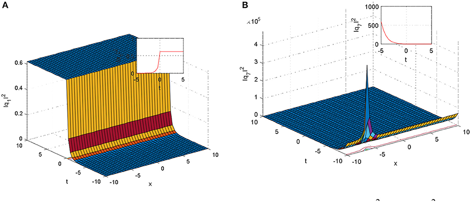
Figure 1. The surface and 2D graphic for the (A) , (B) .
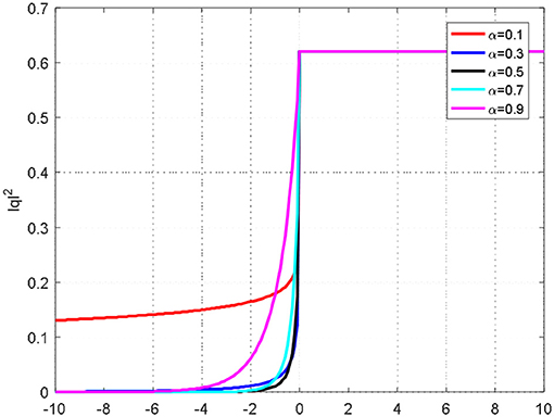
Figure 2. The 2D graphic of the (3+1)-dimensional NLSE with kerr law non-linearities for a different value of α.
The above graphics were drawn for in (a) and for in (b).
We obtained the sum of solutions found for the fractional (3+1)-dimensional NLSE with kerr law nonlinearities via the conformable fractional derivative operator. In addition, we presented some graphics of solutions in Figures 1, 2.
Conclusion
In this article, the EDAM is applied to find new soliton solutions for the (3+1)-dimensional NLSE with kerr law nonlinearities, with the aid of the conformable fractional derivative operator. The dark, bright, and combined optical solitons are obtained. There are 12 different situations in these solutions. The existence of solutions obtained from these functions are all stipulated through limitation states that are also listed in addition to the solutions. Some interesting figures are also presented in Figures 1, 2. The method applied in this article is appropriate to investigate several problems that are face in the fields of engineering and science.
Author Contributions
All authors listed have made a substantial, direct and intellectual contribution to the work, and approved it for publication.
Conflict of Interest
The authors declare that the research was conducted in the absence of any commercial or financial relationships that could be construed as a potential conflict of interest.
Acknowledgments
The authors extend their appreciation to the Deanship of Scientific Research at King Saud University for funding this work through research group no (RG-1440-010).
References
1. Osman MS, Lu D, Khater MMA. A study of optical wave propagation in the nonautonomous Schrodinger-Hirota equation with power-law nonlinearity. Results Phys. (2019) 13:102157. doi: 10.1016/j.rinp.2019.102157
2. Inc M, Korpinar ZS, Al Qurashi MM, Baleanu D. A new method for approximate solution of some nonlinear equations: residual power series method. Adv Mech Eng. (2016) 8:1–7. doi: 10.1177/1687814016644580
3. Khater MMA, Attia RAM, Lu D. Explicit lump solitary wave of certain interesting (3+ 1)-dimensional waves in physics via some recent traveling wave methods. Entropy. (2019) 21:397. doi: 10.3390/e21040397
4. Jana S, Konar S. A new family of Thirring type optical spatial solitons via electromagnetic induced transparency. Phys Lett A. (2007) 362:435–38. doi: 10.1016/j.physleta.2006.10.043
5. Bhrawy AH, Abdelkawy MA. Computational study of some nonlinear shallow water equations. Cent Eur Phys J. (2013) 11:518–25. doi: 10.2478/s11534-013-0197-1
6. Bhrawy AH, Abdelkawy MA. Integrable system modeling shallow water waves: Kaup–Boussinesq shallow water system. Indian Phys J. (2013) 87:665–71. doi: 10.1007/s12648-013-0260-1
7. Biswas A, Milovic D. Optical solitons in 1+2 dimensions with non-Kerr law nonlinearity, Eur Phys Spec Top J. (2009) 173:81–6. doi: 10.1140/epjst/e2009-01068-8
8. Rezazadeh H. New solitons solutions of the complex Ginzburg-Landau equation with Kerr law nonlinearity. Optik. (2018) 167:218–27. doi: 10.1016/j.ijleo.2018.04.026
9. Triki H, Wazwaz AM. Combined optical solitary waves of the Fokas-Lenells equation. Waves Random Complex Media. (2017) 27:587–93. doi: 10.1080/17455030.2017.1285449
10. Inc M, Isa Aliyu A, Yusuf A, Baleanu D. Optical solitons and modulation instability analysis with (3+1)-dimensional nonlinear Shrödinger equation. Superlattices Microstruct. (2017) 112:296–302. doi: 10.1016/j.spmi.2017.09.038
11. Seadawy AR. Stability analysis solutions for nonlinear three-dimensional modified Korteweg–de Vries–Zakharov–Kuznetsov equationin a magnetize delectron–positron plasma. Phys A. (2016) 455:44–51. doi: 10.1016/j.physa.2016.02.061
12. Seadawy AR. Three-dimensional weakly nonlinear shallow water waves regime and its traveling wave solutions. Int J Comput Methods. (2018) 15:1850017. doi: 10.1142/S0219876218500172
13. Ghosh S, Nandy S. Inverse scattering method and vector higher order non-linear Schrödinger equation. Nucl Phys B. (1999) 561:451–66. doi: 10.1016/S0550-3213(99)00484-8
14. Irwaq IA, Alquran M, Jaradat I, Baleanu D. New dual-mode Kadomtsev–Petviashvili model with strong–weak surface tension: analysis and application. Adv Diff Equat. (2018) 2018:433. doi: 10.1186/s13662-018-1893-3
15. Alquran M, Jaradat I, Baleanu D. Shapes and dynamics of dual-mode Hirota–Satsuma coupled KdV equations: exact traveling wave solutions and analysis. Chin J Phys. (2019) 58:49–56. doi: 10.1016/j.cjph.2019.01.005
16. Alquran M, Al-Khaled K, Sivasundaram S, Jaradat HM. Mathematical and numerical study of existence of bifurcations of the generalized fractional Burgers-Huxley equation. Nonlinear Stud. (2017) 24:235–44.
17. Jaradat I, Alquran M, Al-Khaled K. An analytical study of physical models with inherited temporal and spatial memory. Eur Phys J Plus. (2018) 133:162. doi: 10.1140/epjp/i2018-12007-1
18. Ali M, Alquran M, Jaradat I. Asymptotic-sequentially solution style for the generalized Caputo time-fractional Newell-Whitehead-Segel system. Adv Diff Equat. (2019) 2019:70. doi: 10.1186/s13662-019-2021-8
19. Imran MA, Aleem M, Riaz MB, Ali R, Khan I. A comprehensive report on convective flow of fractional (ABC) and (CF) MHD viscous fluid subject to generalized boundary conditions. Chaos Solitons Fractals. (2019) 118:274–89. doi: 10.1016/j.chaos.2018.12.001
20. Asif NA, Hammouch Z, Riaz MB, Bulut H. Analytical solution of a Maxwell fluid with slip effects in view of the Caputo-Fabrizio derivative. Eur Phys J Plus. (2018) 133:272. doi: 10.1140/epjp/i2018-12098-6
21. Riaz MB, Zafar AA. Exact solutions for the blood flow through a circular tube under the influence of a magnetic field using fractional Caputo-Fabrizio derivatives. Mathem Model Nat Phenom. (2018) 13:14. doi: 10.1051/mmnp/2018005
22. Korpinar ZS, Inc M. Numerical simulations for fractional variation of (1+ 1)-dimensional Biswas-Milovic equation. Optik. (2018) 166:77–85. doi: 10.1016/j.ijleo.2018.02.099
23. Tchier F, Inc M, Korpinar ZS, Baleanu D. Solution of the time fractional reaction-diffusion equations with residual power series method. Adv Mech Eng. (2016) 8:1–10. doi: 10.1177/1687814016670867
24. Korpinar Z. On numerical solutions for the Caputo-Fabrizio fractional heat-like equation. Thermal Sci. (2018) 22:87–95. doi: 10.2298/TSCI170614274K
25. Alquran M, Jaradat I, Al-Shara S, Awawdeh F. A new simplified bilinear method for the n-soliton solutions for a generalized FmKdV equation with time-dependent variable coefficients. Int J Nonlinear Sci Num Simul. (2015) 16:259–69. doi: 10.1515/ijnsns-2014-0023
26. Rezazadeh H, Tariq H, Eslami M, Mirzazadeh M, Zhou Q. New exact solutions of nonlinear conformable time-fractional Phi-4 equation. Chin J Phys. (2018) 56:2805–16. doi: 10.1016/j.cjph.2018.08.001
27. Korkmaz A. Explicit exact solutions to some one dimensional conformable time fractional equations. Waves Random Complex Media. (2019) 29:124–37. doi: 10.1080/17455030.2017.1416702
28. Khalil R, Al Horani M, Yousef A, Sababheh M. A new definition of fractional derivative. J Comput Appl Math. (2014) 264:65–70. doi: 10.1016/j.cam.2014.01.002
29. Eslami M, Rezazadeh H. The first integral method for Wu-Zhang system with conformable time-fractional derivative. Calcolo. (2016) 53:475–85. doi: 10.1007/s10092-015-0158-8
30. Çenesiz Y, Baleanu D, Kurt A, Tasbozan O. New exact solutions of Burgers' type equations with conformable derivative. Waves Random Complex Media. (2017) 27:103–16. doi: 10.1080/17455030.2016.1205237
31. Eslami M, Khodadad FS, Nazari F, Rezazadeh H. The first integral method applied to the Bogoyavlenskii equations by means of conformable fractional derivative. Opt Quant Electron. (2017) 49:391. doi: 10.1007/s11082-017-1224-z
32. Rezazadeh H, Manaan J, Khodadad FS, Nazari F. Traveling wave solutions for density-dependent conformable fractional diffusion-reaction equation by the rst integral method and the improved tan(φ(ξ)/2)-expansion method. Opt Quant Electron. (2018) 50:12. doi: 10.1007/s11082-018-1388-1
33. Hosseini Mayeli P, Ansari R. Bright and singular soliton solutions of the conformable time-fractional Klein-Gordon equations with different nonlinearities. Waves Random Complex Media. (2018) 28:426–34. doi: 10.1080/17455030.2017.1362133
Keywords: optical solitons, nonlinear Shrödinger equation, conformable derivative, Kerr law nonlinearity, the extended direct algebraic method
Citation: Korpinar Z, Tchier F and Inc M (2020) On Optical Solitons of the Fractional (3+1)-Dimensional NLSE With Conformable Derivatives. Front. Phys. 8:87. doi: 10.3389/fphy.2020.00087
Received: 11 November 2019; Accepted: 11 March 2020;
Published: 17 April 2020.
Edited by:
Wen-Xiu Ma, University of South Florida, United StatesReviewed by:
Aly R. Seadawy, Taibah University, Saudi ArabiaKashif Ali, COMSATS Institute of Information Technology, Pakistan
Copyright © 2020 Korpinar, Tchier and Inc. This is an open-access article distributed under the terms of the Creative Commons Attribution License (CC BY). The use, distribution or reproduction in other forums is permitted, provided the original author(s) and the copyright owner(s) are credited and that the original publication in this journal is cited, in accordance with accepted academic practice. No use, distribution or reproduction is permitted which does not comply with these terms.
*Correspondence: Mustafa Inc, minc@firat.edu.tr