A Variety of Novel Exact Solutions for Different Models With the Conformable Derivative in Shallow Water

For different nonlinear time-conformable derivative models, a versatile built-in gadget, namely the generalized exp(−φ(ξ))-expansion (GEE) method, is devoted to retrieving different categories of new explicit solutions. These models include the time-fractional approximate long-wave equations, the time-fractional variant-Boussinesq equations, and the time-fractional Wu-Zhang system of equations. The GEE technique is investigated with the help of fractional complex transform and conformable derivative. As a result, we found four types of exact solutions involving hyperbolic function, periodic function, rational functional, and exponential function solutions. The physical significance of the explored solutions depends on the choice of arbitrary parameter values. Finally, we conclude that the GEE method is more effective in establishing the explicit new exact solutions than the exp(−φ(ξ))-expansion method.

Introduction

Analytical solutions of the non-linear partial differential equation (NPDEs) are significantly more important for describing the physical meaning for any real-world problems. Due to the rapid expansion of computer technologies and computer-based symbolic tools, researchers have concentrated increasingly on the analytical and numerical solutions for the NPDEs, including integer and fractional orders. During recent decades, several analytical and semi-analytical methods, such as the improved fractional sub-equation [1], the exp function method [2, 3], the G′/G-expansion [4–7], the tan(Φ(ξ)/2)-expansion [8], the modified Kudryashov [9, 10], the new extended direct algebraic [11], the extended exp(−φ(ξ))-expansion [12], the RB sub-ODE [13], the sine-Gordon expansion [14–16], the unified [17, 18], and the generalized unified [19, 20] methods, have been investigated and also employed for acquiring the new exact solutions of the well-known NPDEs that arise in applied sciences. Presenting new exact solution of PDEs provides a better understanding of the phenomena, which are governed by three special form of time-fractional WKB equations.

The time-fractional Whitham-Broer-Kaup (WBK) equation has the following structure [21]

$\begin{array}{ll}\begin{array}{c}{D}_t^{\alpha }u+u{u}_x+v_x+\beta u_{xx}=0\\ D_t^{\alpha }v+{(uv)}_x-\beta v_{xx}+\gamma u_{xxx}=0\end{array}\},t\ge 0,0<\alpha \le 1.& (1)\end{array}$

Eq. (1) describes the dispersive long wave in shallow water [22] where u = u(x, t) is the velocity field in the horizontal direction, v = v(x, t) is he height which deviates from the liquid balance position, and β and γ are real parameters [23]. $D_t^{\alpha }(.)$ is conformable derivative of order α. In the past, many researchers studied the WBK equation via different analytical approaches according to their field, particularly within mathematical physics and ocean engineering. For instance, Guo et al. [24] employed the improved sub-equation method to extract analytical solutions for space- and time-fractional WBK equations. El-Borai et al. [25] applied the exp-function method under the sense of the modified Riemann-Liouville derivative for solving the time-fractional coupled WBK equations.

If we choose the free parameters as $\beta =\frac{1}{2}$ and γ = 0, Eq. (1) is converted to the time-fractional approximate long-wave equations [21]:

$\begin{array}{ll}\begin{array}{c}{D}_t^{\alpha }u+u{u}_x+v_x+\frac{1}{2}{u}_{xx}=0\\ D_t^{\alpha }v+{(uv)}_x-\frac{1}{2}{v}_{xx}=0\\ \end{array}\},t\ge 0,0<\alpha \le 1.& (2)\end{array}$

In past, Eq. (2) have been solved by the fractional sub-equation method [26], the G′/G-expansion method [24], and the generalized Kudryashov method [27] for establishing different wave solutions.

Again, we substitute β = 0 and γ = 1 in Eq. (1), and Eq. (1) is converted to the following time-fractional variant Boussinesq equations [21]:

$\begin{array}{ll}\begin{array}{c}{D}_t^{\alpha }u+u{u}_x+v_x=0\\ D_t^{\alpha }v+{(uv)}_x+u_{xxx}=0\\ \end{array}\},t\ge 0,0<\alpha \le 1.& (3)\end{array}$

Equation (3) was solved by Yan [26] by using fractional sub-equation method. The improved fractional sub-equation method [24] was applied for producing the new generalized exact solutions of the space–time-fractional variant Boussinesq equations.

Finally, if we choose the free parameter values β = 0 and $\gamma =\frac{1}{3}$ in Eq. (1), Eq. (1) is the converted to the following time-fractional Wu-Zhang system of equations [27]:

$\begin{array}{ll}\begin{array}{c}{D}_t^{\alpha }u+u{u}_x+v_x=0\\ D_t^{\alpha }v+{(uv)}_x+\frac{1}{3}{u}_{xxx}=0\end{array}\},t\ge 0,0<\alpha \le 1.& (4)\end{array}$

Eslami et al. [27] solved the time-fractional Wu-Zhang system of equations using the first integral method by considering conformable fractional sense.

If we consider α = 1in Eq. (1), then it is converted to the classical coupled WBK equation, which was first introduced by Whitham [28], Broer [29], and Kaup [30]. When α = 1, β ≠ 0, and γ = 1, Eq. (1) is the classical long-wave equation that describes the shallow water wave with diffusion. When α = 1, β = 0, and γ = 1, Eq. (1) reduces the classical variant Boussinesq equations [31], and when α = 1, β = 0 and γ = 1/3, Eq. (1) reduces the classical Wu-Zhang system of equations [32]. Sometimes, the classical Wu-Zhang system of equations are introduced by the (1+1) dimensional dispersive long-wave equations [33–35].

For the simplicity of the solutions, we did not consider solving the time-fractional WKB equations by the generalized exp(−φ(ξ))-expansion method. The main aim of this work is to construct the new exact traveling wave solutions of the three-special form of time-fractional WKB equations, such as the time-fractional approximate long-wave equations, the time-fractional variant Boussinesq equations, and the time-fractional Wu-Zhang system of equations using the generalized exp(−φ(ξ))- expansion method with a conformable derivative sense. The generalized exp(−φ(ξ))-expansion method is an effectual and easily applicable technique that is used to investigate the new exact solution for different integer- and fractional-order PDEs. Very recently, Lu et al. [36] used the generalized exp(−φ(ξ))- expansion method and construct the exact solutions of space–time-fractional generalized fifth-order KdV equation with Jumarie's modified Riemann-Liouville derivatives.

The rest of the paper is arranged as follows. In section Conformable derivative and the generalized exp(−φ(ξ))-expansion method, some basic definitions of conformable derivative and the main steps of the generalized exp(−φ(ξ))-expansion method are given. In section Application of the generalized exp(−φ(ξ))-expansion method, we look for the exact solutions of Eq. (2) to Eq. (4) via the generalized exp(−φ(ξ))-expansion method. Finally, a brief conclusion is provided in the last section.

The Conformable Derivative and the Generalized exp(−φ(ξ))-Expansion Method

Khalil et al. [37] started to give us the first definition of the conformable derivative (CD) with a limit operator as follows.

Definition 1. If f : (0, ∞) → R, then the CFD of f order α is defined as

$\begin{array}{l}{D}_t^{\alpha }f(t)={\displaystyle \underset{\epsilon \to 0}{\text{lim}}}\frac{f\left(t+\epsilon t^{1-\alpha }\right)-f(t)}{\epsilon },\text{ for all t}>0,0<\alpha \le 1.\end{array}$

The CD satisfies some workable features that are demonstrated in the following theorems [37–41].

Theorem 1. Let α ∈ (0, 1] and f = f(t), g = g(t) be α-conformable differentiable at a point t > 0, then

$\begin{array}{l}(i)D_t^{\alpha }(af+bg)=a{D}_t^{\alpha }f+b{D}_t^{\alpha }g,foralla,b\in R,\\ (ii)D_t^{\alpha }(t^{\mu })=\mu t^{\mu -\alpha },forall\mu \in R,\\ (iii)D_t^{\alpha }(fg)=g{D}_t^{\alpha }(f)+f{D}_t^{\alpha }(g),\\ (iv)D_t^{\alpha }\left(\frac{f}{g}\right)=\frac{g{D}_t^{\alpha }(f)-f{D}_t^{\alpha }(g)}{g^2}.\end{array}$

Furthermore, if f is differentiable, then $D_t^{\alpha }\left(f(t)\right)=t^{1-\alpha }\frac{df}{dt}$.

Theorem 2. Let f : (0, ∝) → R be a function such that f is differentiable and α-conformable differentiable. Also, let g be a differentiable function defined in the range of f. Then

$\begin{array}{l}{D}_t^{\alpha }(fog)(t)=t^{1-\alpha }{g(t)}^{\alpha -1}{g}^{\prime }(t)D_t^{\alpha }{(f(t))}_{t=g(t)}\end{array}$

where prime denotes the classical derivatives with respect to t.

Now, we impose the generalized exp(−φ(ξ))-expansion method for solving some fractional differential equations. In this respect, we described the essential steps of the generalized exp(−φ(ξ))- expansion method [36] as follows.

Step-1: Suppose that a general form of the non-linear FDEs, say in two independent variables x and t, is given by

$\begin{array}{l}\begin{array}{c}{P}_1\left(u,v,D_t^{\alpha }u,D_t^{\alpha }v,D_t^{2\alpha }u,D_t^{2\alpha }v,u_x,v_x,u_{xx},v_{xx},\dots \dots \right)=0\\ P_2\left(u,v,D_t^{\alpha }u,D_t^{\alpha }v,D_t^{2\alpha }u,D_t^{2\alpha }v,u_x,v_x,u_{xx},v_{xx},\dots \dots \right)=0\\ \end{array}\}\\ \begin{array}{l},0<\alpha \le 1,t>0,\end{array}& (5)\end{array}$

where $D_t^{\alpha }u$ and $D_t^{\alpha }v$ are conformable derivatives of u and v, respectively, u = u(x, t) and v = v(x, t) are an unknown functions, and P₁ and P₂ are a polynomial in their arguments.

Step-2: To construct the exact solution of Eq. (5), we introduce the variable transformation, combine the real variables x and t by a compound variable ξ

$\begin{array}{ll}u=U(\xi )\text{ and }v=V(\xi ),\xi =x-\left(\frac{c}{\alpha }\right)t^{\alpha },& (6)\end{array}$

where, c is a constant which is determined later. The traveling wave transformation of Eq. (6) converts Eq. (5) into an ordinary differential equation (ODE) for u = U(ξ) and v = V(ξ):

$\begin{array}{ll}\begin{array}{c}{Q}_1\left(U,{V,U}^{\prime },V^{\prime },U^{″},V^{″},\dots \dots \right)=0\\ Q_1\left(U,{V,U}^{\prime },V^{\prime },U^{″},V^{″},\dots \dots \right)=0\end{array}\},& (7)\end{array}$

where Q₁and Q₂ are a polynomial of U, V, and its derivatives with respect to ξ.

Step 3: Suppose that the traveling wave solution of system Eq. (7) can be presented as follows

$\begin{array}{ll}\begin{array}{c}U(\xi )={\text{a}}_0+{\sum }_{i=1}^m{a}_i{\left(exp(-\phi (\xi ))\right)}^i\\ V(\xi )=b_0+{\sum }_{i=1}^n{\text{b}}_{\text{i}}{\left(exp(-\phi (\xi ))\right)}^i\end{array}\},& (8)\end{array}$

where the arbitrary constants a_i(i = 1, 2…, m) and b_i(i = 1, 2…, n) are determined latter, but a_m ≠ 0 and b_n ≠ 0 and also m and n are a positive integer, which can be determined by using homogeneous balance principle on Eq. (7), and φ = φ(ξ) satisfies the following new ansatz equation

$\begin{array}{ll}{\phi }^{\prime }(\xi )=pexp(-\phi (\xi ))+qexp(\phi (\xi ))+r& (9)\end{array}$

where p, q, and r are constant. The general solutions of the equation are the following.

Case-I: When p = 1 and Δ = r² − 4q, one obtains

$\begin{array}{ll}\begin{array}{c}\phi (\xi )=\text{ln}\left(\frac{-\sqrt{\Delta }\text{tanh}\left(\frac{1}{2}\sqrt{\Delta }(\xi +E)\right)-r}{2q}\right),q\ne 0,\\ \Delta =r^2-4q>0\\ \phi (\xi )=\text{ln}\left(\frac{-\sqrt{\Delta }\text{coth}\left(\frac{1}{2}\sqrt{\Delta }(\xi +E)\right)-r}{2q}\right),q\ne 0,\\ \Delta =r^2-4q>0\end{array}\},& (10)\end{array}$

$\begin{array}{ll}\begin{array}{c}\phi (\xi )=\text{ln}\left(\frac{\sqrt{-\Delta }\text{tan}\left(\frac{1}{2}\sqrt{-\Delta }(\xi +E)\right)-r}{2q}\right),q\ne 0,\\ \Delta =r^2-4q<0\\ \phi (\xi )=\text{ln}\left(\frac{\sqrt{-\Delta }\text{cot}\left(\frac{1}{2}\sqrt{-\Delta }(\xi +E)\right)-r}{2q}\right),q\ne 0,\\ \Delta =r^2-4q<0\end{array}\},& (11)\end{array}$

$\begin{array}{l}\phi (\xi )=-\text{ln}\left(\frac{r}{exp(r(\xi +E))-1}\right),\\ \begin{array}{l}q=0,r\ne 0,=r^2-4q>0,\end{array}& (12)\end{array}$

and

$\begin{array}{l}\phi (\xi )=\text{ln}\left(-\frac{2(r(\xi +E)+2)}{r^2(\xi +E)}\right),\\ \begin{array}{l}q\ne 0,r\ne 0,\Delta =r^2-4q=0.\end{array}& (13)\end{array}$

Case-II: When r = 0, one obtains

$\begin{array}{ll}\phi (\xi )=\text{ln}\left(\sqrt{\frac{p}{q}}tan\left(\sqrt{pq}(\xi +E)\right)\right),p>0,q>0.& (14)\end{array}$

$\begin{array}{ll}\phi (\xi )=\text{ln}\left(-\sqrt{\frac{p}{q}}cot\left(\sqrt{pq}(\xi +E)\right)\right),p<0,q<0.& (15)\end{array}$

$\begin{array}{l}\phi (\xi )=\text{ln}\left(\sqrt{-\frac{p}{q}}tanh\left(\sqrt{-pq}(\xi +E)\right)\right),\\ \begin{array}{l}p>0,q<0.\end{array}& (16)\end{array}$

$\begin{array}{l}\phi (\xi )=\text{ln}\left(-\sqrt{-\frac{p}{q}}coth\left(\sqrt{-pq}(\xi +E)\right)\right),\\ \begin{array}{l}p<0,q>0.\end{array}& (17)\end{array}$

Case-III: When q = 0 and r = 0, one obtains

$\begin{array}{ll}\phi (\xi )=\text{ln}\left(p(\xi +E)\right).& (18)\end{array}$

For all cases, E is the integrating constant.

Step 4: Inserting Eq. (9) in Eq. (8) and compiling the terms in the resulting equation yields a set of algebraic non-linear equations. Finally, by solving this set we reach the exact solutions of the non-linear fractional PDEs.

Application of the Generalized exp(−φ(ξ))-Expansion Method

In this part, we will execute the generalized exp(−φ(ξ))- expansion method to solve three well-known non-linear fractional partial differential equations in shallow water, namely, the time-fractional approximate long wave (ALW) equations, the time-fractional variant-Boussinesq equations, and the time-fractional Wu-Zhang system of equations. All the above mentioned equations are the special-form WBK equations that describe the physical phenomena arising in fluid mechanics.

The Time-Fractional ALW Equations

Let us consider the time-fractional ALW equations

$\begin{array}{ll}\begin{array}{c}{D}_t^{\alpha }u+u{u}_x+v_x+\frac{1}{2}{u}_{xx}=0\\ D_t^{\alpha }v+{(uv)}_x-\frac{1}{2}{v}_{xx}=0\end{array}\},t\ge 0,0<\alpha \le 1.& (19)\end{array}$

Now, applying under the traveling wave transformation of Eq. (6), Eq. (19) reduces to a non-linear ODE as

$\begin{array}{ll}\begin{array}{c}-c{U}^{\prime }+U{U}^{\prime }+V^{\prime }+\frac{1}{2}{U}^{″}=0\\ -c{V}^{\prime }+{(UV)}^{\prime }-\frac{1}{2}{V}^{″}=0\end{array}\}.& (20)\end{array}$

This integrates with respect to ξ of Eq. (20) and considers that the integration constant is zero. Eq. (20) then yields

$\begin{array}{ll}\begin{array}{c}-cU+\frac{1}{2}{U}^2+V+\frac{1}{2}{U}^{\prime }=0\\ -cV+UV-\frac{1}{2}{V}^{\prime }=0\end{array}\}.& (21)\end{array}$

The balancing rule in Eq. (21) yields m = 1 and n = 2, assuming the general solution Eq. (21) in the presence Eq. (8) is given by

$\begin{array}{ll}\begin{array}{c}U(\xi )=a_0+a_{1}exp(-\phi (\xi ))\\ V(\xi )=b_0+b_{1}exp(-\phi (\xi ))+b_{2}exp(-2\phi (\xi ))\end{array}\},& (22)\end{array}$

where a₁ ≠ 0 and b₂ ≠ 0.

Plugging Eq. (22) into Eq. (21), we obtain a set of an algebraic non-linear equations that solve to

Set-1: $a_0=-\frac{1}{2}r+\frac{1}{2}\sqrt{-4pq+r^2},a_1=-p,b_0=-pq,b_1=-pr,b_2=-p^2$

$\text{and }c=\frac{1}{2}\sqrt{-4pq+r^2},-4pq+r^2>0$.

By putting the values of Set-1 into Eq. (22) along with the Eq. (10) to Eq. (18), we obtain the following traveling wave solutions for the time-fractional ALW equations.

For p = 1:

$\begin{array}{ll}\begin{array}{c}{u}_1(x,t)=-\frac{1}{2}r+\frac{1}{2}\sqrt{r^2-4q}\\ +\frac{2q}{\sqrt{\Delta }\text{ tan }h\left(\frac{1}{2}\sqrt{\Delta }(\xi +E)\right)+r}\\ v_1(x,t)=-q+\frac{2rq}{\sqrt{\Delta }\text{ tan }h\left(\frac{1}{2}\sqrt{\Delta }(\xi +E)\right)+r}\\ -\frac{4q^2}{{(\sqrt{\Delta }\text{ tan }h\left(\frac{1}{2}\sqrt{\Delta }(\xi +E)\right)+r)}^2}\end{array}\},& (23)\end{array}$

$\begin{array}{ll}\begin{array}{c}{u}_2(x,t)=-\frac{1}{2}r+\frac{1}{2}\sqrt{r^2-4q}\\ +\frac{2q}{\sqrt{\Delta }\text{ cot }h\left(\frac{1}{2}\sqrt{\Delta }(\xi +E)\right)+r}\\ v_2(x,t)=-q+\frac{2rq}{\sqrt{\Delta }\text{ cot }h\left(\frac{1}{2}\sqrt{}(\xi +E)\right)+r}\\ -\frac{4q^2}{{(\sqrt{\Delta }\text{ cot }h\left(\frac{1}{2}\sqrt{\Delta }(\xi +E)\right)+r)}^2}\end{array}\},& (24)\end{array}$

$\begin{array}{ll}\begin{array}{c}{u}_3(x,t)=-\frac{1}{2}r+\frac{1}{2}\sqrt{r^2-4q}\\ -\frac{2q}{\sqrt{-\Delta }\text{ tan}\left(\frac{1}{2}\sqrt{-\Delta }(\xi +E)\right)-r}\\ v_3(x,t)=-q-\frac{2rq}{\sqrt{-\Delta }\text{ tan}\left(\frac{1}{2}\sqrt{-\Delta }(\xi +E)\right)-r}\\ -\frac{4q^2}{{(\sqrt{-\Delta }\text{ tan}\left(\frac{1}{2}\sqrt{-\Delta }(\xi +E)\right)-r)}^2}\end{array}\},& (25)\end{array}$

$\begin{array}{ll}\begin{array}{c}{u}_4(x,t)=-\frac{1}{2}r+\frac{1}{2}\sqrt{r^2-4q}\\ -\frac{2q}{\sqrt{-\Delta }\text{ cot}\left(\frac{1}{2}\sqrt{-\Delta }(\xi +E)\right)-r}\\ v_4(x,t)=-q-\frac{2rq}{\sqrt{-\Delta }\text{ cot}\left(\frac{1}{2}\sqrt{-\Delta }(\xi +E)\right)-r}\\ -\frac{4q^2}{{(\sqrt{-\Delta }\text{ cot}\left(\frac{1}{2}\sqrt{-\Delta }(\xi +E)\right)-r)}^2}\end{array}\},& (26)\end{array}$

$\begin{array}{ll}\begin{array}{c}{u}_5(x,t)=-\frac{1}{2}r+\frac{1}{2}\sqrt{r^2-4q}-\frac{r}{e^{r(\xi +E)}-1}\\ v_5(x,t)=-q-\frac{r^2}{e^{r(\xi +E)}-1}-\frac{r^2}{{(e^{r(\xi +E)}-1)}^2}\end{array}\},& (27)\end{array}$

and

$\begin{array}{ll}\begin{array}{c}{u}_6(x,t)=-\frac{1}{2}r+\frac{1}{2}\sqrt{r^2-4q}+\frac{1}{2}\frac{r^2(\xi +E)}{r(\xi +E)+2}\\ v_6(x,t)=-q+\frac{1}{2}\frac{r^3(\xi +E)}{r(\xi +E)+2}-\frac{1}{4}{\left(\frac{r^2(\xi +E)}{r(\xi +E)+2}\right)}^2\end{array}\},& (28)\end{array}$

where, $\xi =x-\left(\frac{1}{2}\sqrt{r^2-4q}\right)\frac{t^{\alpha }}{\alpha }$ and = r² − 4q > 0.

For r = 0:

$\begin{array}{ll}\begin{array}{c}{u}_7(x,t)=\frac{1}{2}\sqrt{-4pq}+\frac{\sqrt{pq}}{\text{tan}\left(\sqrt{pq}(\xi +E)\right)}\\ v_7(x,t)=-pq-{\left(\frac{\sqrt{pq}}{\text{tan}\left(\sqrt{pq}(\xi +E)\right)}\right)}^2\end{array}\},& (29)\end{array}$

$\begin{array}{ll}\begin{array}{c}{u}_8(x,t)=\frac{1}{2}\sqrt{-4pq}+\frac{\sqrt{pq}}{\text{cot}\left(\sqrt{pq}(\xi +E)\right)}\\ v_8(x,t)=-pq-{\left(\frac{\sqrt{pq}}{\text{cot}(\sqrt{pq}(\xi +E))}\right)}^2\end{array}\},& (30)\end{array}$

$\begin{array}{ll}\begin{array}{c}{u}_9(x,t)=\frac{1}{2}\sqrt{-4pq}-\frac{\sqrt{-pq}}{\text{tanh}\left(\sqrt{-pq}(\xi +E)\right)}\\ v_9(x,t)=-pq+{\left(\frac{\sqrt{pq}}{\text{tanh}(\sqrt{pq}(\xi +E))}\right)}^2\end{array}\},& (31)\end{array}$

and

$\begin{array}{ll}\begin{array}{c}{u}_{10}(x,t)=\frac{1}{2}\sqrt{-4pq}+\frac{\sqrt{-pq}}{\text{coth}\left(\sqrt{-pq}(\xi +E)\right)}\\ v_{10}(x,t)=-pq+{\left(\frac{\sqrt{pq}}{\text{coth}(\sqrt{-pq}(\xi +E))}\right)}^2\end{array}\},& (32)\end{array}$

where, $\xi =x-\left(\frac{1}{2}\sqrt{-4pq}\right)\frac{t^{\alpha }}{\alpha },pq<0$.

For q = 0 and r = 0:

$\begin{array}{ll}\begin{array}{c}{u}_{11}(x,t)=-\frac{1}{x+E}\\ v_{11}(x,t)=-{\left(\frac{1}{x+E}\right)}^2\end{array}\},& (33)\end{array}$

Set-2: $a_0=-\frac{1}{2}r-\frac{1}{2}\sqrt{-4pq+r^2},a_1=-p,b_0=-pq,b_1=-pr,b_2=-p^2$

$\text{and }c=-\frac{1}{2}\sqrt{-4pq+r^2},-4pq+r^2>0$.

Consequently, by substituting the values of Set-2 into Eq. (22) along with the Eq. (10) to Eq. (18), we produce the following traveling wave solutions for the time-fractional ALW equations.

For p = 1:

$\begin{array}{ll}\begin{array}{c}{u}_{12}(x,t)=-\frac{1}{2}r-\frac{1}{2}\sqrt{r^2-4q}\\ +\frac{2q}{\sqrt{\Delta }\text{ tan }h\left(\frac{1}{2}\sqrt{\Delta }(\xi +E)\right)+r}\\ v_{12}(x,t)=-q+\frac{2rq}{\sqrt{\Delta }\text{ tan }h\left(\frac{1}{2}\sqrt{\Delta }(\xi +E)\right)+r}\\ -\frac{4q^2}{{\left(\sqrt{\Delta }\text{ tan }h(\frac{1}{2}\sqrt{\Delta }(\xi +E))+r\right)}^2}\end{array}\},& (34)\end{array}$

$\begin{array}{ll}\begin{array}{c}{u}_{13}(x,t)=-\frac{1}{2}r-\frac{1}{2}\sqrt{r^2-4q}\\ +\frac{2q}{\sqrt{\Delta }\text{ cot }h\left(\frac{1}{2}\sqrt{\Delta }(\xi +E)\right)+r}\\ v_{13}(x,t)=-q+\frac{2rq}{\sqrt{\Delta }\text{ cot }h\left(\frac{1}{2}\sqrt{\Delta }(\xi +E)\right)+r}\\ -\frac{4q^2}{{\left(\sqrt{\Delta }\text{ cot }h\left(\frac{1}{2}\sqrt{\Delta }(\xi +E)\right)+r\right)}^2}\end{array}\},& (35)\end{array}$

$\begin{array}{ll}\begin{array}{c}{u}_{14}(x,t)=-\frac{1}{2}r-\frac{1}{2}\sqrt{r^2-4q}\\ -\frac{2q}{\sqrt{-\Delta }\text{ tan}\left(\frac{1}{2}\sqrt{-\Delta }(\xi +E)\right)-r}\\ v_{14}(x,t)=-q-\frac{2rq}{\sqrt{-\Delta }\text{ tan}\left(\frac{1}{2}\sqrt{-}(\xi +E)\right)-r}\\ -\frac{4q^2}{{(\sqrt{-\Delta }\text{ tan}\left(\frac{1}{2}\sqrt{-\Delta }(\xi +E)\right)-r)}^2}\end{array}\},& (36)\end{array}$

$\begin{array}{ll}\begin{array}{c}{u}_{15}(x,t)=-\frac{1}{2}r-\frac{1}{2}\sqrt{r^2-4q}\\ -\frac{2q}{\sqrt{-\Delta }\text{ cot}\left(\frac{1}{2}\sqrt{-\Delta }(\xi +E)\right)-r}\\ v_{15}(x,t)=-q-\frac{2rq}{\sqrt{-\Delta }\text{ cot}\left(\frac{1}{2}\sqrt{-\Delta }(\xi +E)\right)-r}\\ -\frac{4q^2}{{(\sqrt{-\Delta }\text{ cot}\left(\frac{1}{2}\sqrt{-\Delta }(\xi +E)\right)-r)}^2}\end{array}\},& (37)\end{array}$

$\begin{array}{ll}\begin{array}{c}{u}_{16}(x,t)=-\frac{1}{2}r-\frac{1}{2}\sqrt{r^2-4q}-\frac{r}{e^{r(\xi +E)}-1}\\ v_{16}(x,t)=-q-\frac{r^2}{e^{r(\xi +E)}-1}-\frac{r^2}{{(e^{r(\xi +E)}-1)}^2}\end{array}\},& (38)\end{array}$

and

$\begin{array}{ll}\begin{array}{c}{u}_{17}(x,t)=-\frac{1}{2}r-\frac{1}{2}\sqrt{r^2-4q}+\frac{1}{2}\frac{r^2(\xi +E)}{r(\xi +E)+2}\\ v_{17}(x,t)=-q+\frac{1}{2}\frac{r^3(\xi +E)}{r(\xi +E)+2}-\frac{1}{4}{\left(\frac{r^2(\xi +E)}{r(\xi +E)+2}\right)}^2\end{array}\},& (39)\end{array}$

where, $\xi =x+\left(\frac{1}{2}\sqrt{r^2-4q}\right)\frac{t^{\alpha }}{\alpha }$ and = r² − 4q > 0.

For r = 0:

$\begin{array}{ll}\begin{array}{c}{u}_{18}(x,t)=-\frac{1}{2}\sqrt{-4pq}-\frac{\sqrt{pq}}{\text{tan}\left(\sqrt{pq}(\xi +E)\right)}\\ v_{18}(x,t)=-pq-{\left(\frac{\sqrt{pq}}{\text{tan}\left(\sqrt{pq}(\xi +E)\right)}\right)}^2\end{array}\},& (40)\end{array}$

$\begin{array}{ll}\begin{array}{c}{u}_{19}(x,t)=-\frac{1}{2}\sqrt{-4pq}+\frac{\sqrt{pq}}{\text{cot}\left(\sqrt{pq}(\xi +E)\right)}\\ v_{19}(x,t)=-pq-{\left(\frac{\sqrt{pq}}{\text{cot}\left(\sqrt{pq}(\xi +E)\right)}\right)}^2\end{array}\},& (41)\end{array}$

$\begin{array}{ll}\begin{array}{c}{u}_{20}(x,t)=-\frac{1}{2}\sqrt{-4pq}-\frac{\sqrt{pq}}{\text{tanh}\left(\sqrt{-pq}(\xi +E)\right)}\\ v_{20}(x,t)=-pq+{\left(\frac{\sqrt{pq}}{\text{tanh}\left(\sqrt{-pq}(\xi +E)\right)}\right)}^2\end{array}\},& (42)\end{array}$

and

$\begin{array}{ll}\begin{array}{c}{u}_{21}(x,t)=-\frac{1}{2}\sqrt{-4pq}+\frac{\sqrt{-pq}}{\text{coth}\left(\sqrt{-pq}(\xi +E)\right)}\\ v_{21}(x,t)=-pq+{\left(\frac{\sqrt{pq}}{\text{coth}(\sqrt{-pq}(\xi +E))}\right)}^2\end{array}\},& (43)\end{array}$

where, $\xi =x+\left(\frac{1}{2}\sqrt{-4pq}\right)\frac{t^{\alpha }}{\alpha },pq<0$.

For q = 0 and r = 0:

$\begin{array}{ll}\begin{array}{c}{u}_{22}(x,t)=-\frac{1}{x+E}\\ v_{22}(x,t)=-{\left(\frac{1}{x+E}\right)}^2\\ \end{array}\},& (44)\end{array}$

Figures 1, 2 represent the solutions given by Eq. (23) for different values of α when r = 3, q = 2, and E = 0.

FIGURE 1

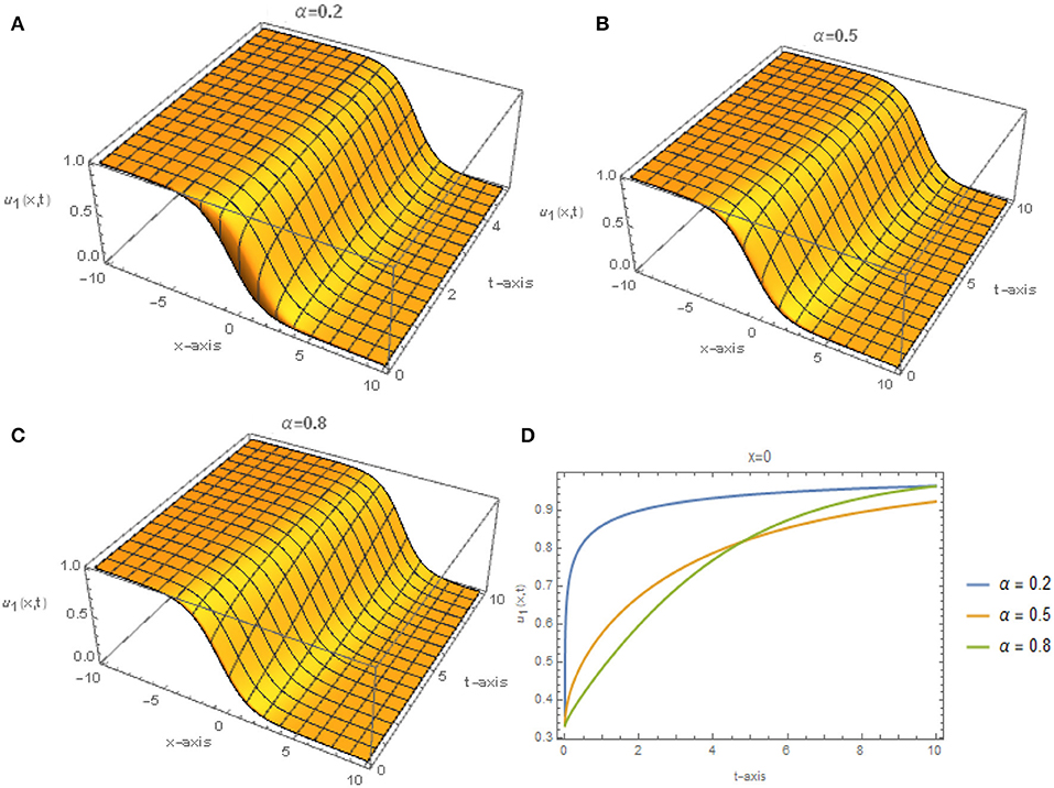
Figure 1. (A–D) The Solution u_1 (x,t) given by Eq. (23).

FIGURE 2

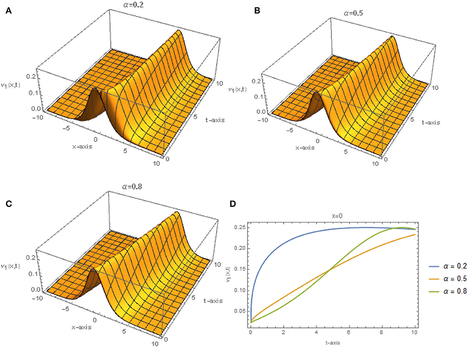
Figure 2. (A–D) The Solution v_1 (x,t) given by Eq. (23).

The Time-Fractional Variant-Boussinesq Equations

Let us consider the time-fractional variant-Boussinesq equations

$\begin{array}{ll}\begin{array}{c}{D}_t^{\alpha }u+u{u}_x+v_x=0\\ D_t^{\alpha }v+{(uv)}_x+u_{xxx}=0\end{array}\},t\ge 0,0<\alpha \le 1.& (45)\end{array}$

Now, applying under the traveling wave transformation of Eq. (6), Eq. (45) reduces to a non-linear ODE as

$\begin{array}{ll}\begin{array}{c}-c{U}^{\prime }+U{U}^{\prime }+V^{\prime }=0\\ -c{V}^{\prime }+{(UV)}^{\prime }+U^{‴}=0\\ \end{array}\}.& (46)\end{array}$

This integrates with respect to ξ of Eq. (46) and considers the integration constant to be zero. Eq. (46) then yields

$\begin{array}{ll}\begin{array}{c}-cU+\frac{1}{2}{U}^2+V=0\\ -cV+UV+U^{″}=0\\ \end{array}\}.& (47)\end{array}$

From the balancing condition in Eq. (47), we have m = 1 and n = 2. Now, the formal solution of (47) in the existence of (8) will be

$\begin{array}{ll}\begin{array}{c}U(\xi )=a_0+a_1\text{exp}(-\phi (\xi ))\\ V(\xi )=b_0+b_1\text{exp}(-\phi (\xi ))+b_2\text{exp}(-2\phi (\xi ))\end{array}\}& (48)\end{array}$

where a₁ ≠ 0 and b₂ ≠ 0.

By inserting Eq. (48) into Eq. (47) along with Eq. (9) and using the same techniques investigated in the previous section we get

Set-1: $a_0=-r\pm \sqrt{-4pq+r^2},a_1=-2p,b_0=-2pq,b_1=-2pr,b_2=-{2p}^2$

$\text{and }c=\pm \sqrt{-4pq+r^2},-4pq+r^2>0$.

Therefore, by substituting the values of Set-1 into Eq. (48), along with the Eq. (10) to Eq. (18), we generate the following traveling wave solutions for the time-fractional variant-Boussinesq equations.

For p = 1:

$\begin{array}{ll}\begin{array}{c}{u}_1(x,t)=-r\pm \sqrt{r^2-4q}\\ +\frac{4q}{\sqrt{\Delta }\text{ tan }h\left(\frac{1}{2}\sqrt{\Delta }(\xi +E)\right)+r}\\ v_1(x,t)=-2q+\frac{4rq}{\sqrt{\Delta }\text{ tan }h\left(\frac{1}{2}\sqrt{\Delta }(\xi +E)\right)+r}\\ -\frac{8q^2}{{\left(\sqrt{\Delta }\text{ tan }h\left(\frac{1}{2}\sqrt{\Delta }(\xi +E)\right)+r\right)}^2}\end{array}\},& (49)\end{array}$

$\begin{array}{ll}\begin{array}{c}{u}_2(x,t)=-r\pm \sqrt{r^2-4q}\\ +\frac{4q}{\sqrt{\Delta }\text{ cot }h\left(\frac{1}{2}\sqrt{\Delta }(\xi +E)\right)+r}\\ v_2(x,t)=-2q+\frac{4rq}{\sqrt{\Delta }\text{ cot }h\left(\frac{1}{2}\sqrt{}(\xi +E)\right)+r}\\ -\frac{8q^2}{{\left(\sqrt{\Delta }\text{ cot }h\left(\frac{1}{2}\sqrt{\Delta }(\xi +E)\right)+r\right)}^2}\end{array}\},& (50)\end{array}$

$\begin{array}{ll}\begin{array}{c}{u}_3(x,t)=-r\pm \sqrt{r^2-4q}\\ -\frac{4q}{\sqrt{-\Delta }\text{ tan}\left(\frac{1}{2}\sqrt{-}(\xi +E)\right)-r}\\ v_3(x,t)=-2q-\frac{4rq}{\sqrt{-\Delta }\text{ tan}\left(\frac{1}{2}\sqrt{-\Delta }(\xi +E)\right)-r}\\ -\frac{8q^2}{{(\sqrt{-\Delta }\text{ tan}\left(\frac{1}{2}\sqrt{-\Delta }(\xi +E)\right)-r)}^2}\end{array}\},& (51)\end{array}$

$\begin{array}{ll}\begin{array}{c}{u}_4(x,t)=-r\pm \sqrt{r^2-4q}\\ -\frac{4q}{\sqrt{-\Delta }\text{ cot}\left(\frac{1}{2}\sqrt{-\Delta }(\xi +E)\right)-r}\\ v_4(x,t)=-2q-\frac{4rq}{\sqrt{-\Delta }\text{ cot}\left(\frac{1}{2}\sqrt{-\Delta }(\xi +E)\right)-r}\\ -\frac{8q^2}{{(\sqrt{-\Delta }\text{ cot}\left(\frac{1}{2}\sqrt{-}(\xi +E)\right)-r)}^2}\end{array}\},& (52)\end{array}$

$\begin{array}{ll}\begin{array}{c}{u}_5(x,t)=-r\pm \sqrt{r^2-4q}-\frac{2r}{e^{r(\xi +E)}-1}\\ v_5(x,t)=-2q-\frac{2r^2}{e^{r(\xi +E)}-1}-\frac{2r^2}{{\left(e^{r(\xi +E)}-1\right)}^2}\end{array}\},& (53)\end{array}$

and

$\begin{array}{ll}\begin{array}{c}{u}_6(x,t)=-r\pm \sqrt{r^2-4q}+\frac{r^2(\xi +E)}{r(\xi +E)+2}\\ v_6(x,t)=-2q+\frac{r^3(\xi +E)}{r(\xi +E)+2}-\frac{1}{2}{\left(\frac{r^2(\xi +E)}{r(\xi +E)+2}\right)}^2\end{array}\}& (54)\end{array}$

where $\xi =x\mp \left(\sqrt{r^2-4q}\right)\frac{t^{\alpha }}{\alpha }$ and = r² − 4q > 0.

For r = 0:

$\begin{array}{ll}\begin{array}{c}{u}_7(x,t)=\pm \sqrt{-4pq}-\frac{2\sqrt{pq}}{\text{tan}\left(\sqrt{pq}(\xi +E)\right)}\\ v_7(x,t)=-2pq-{\left(\frac{\sqrt{2pq}}{\text{tan}\left(\sqrt{pq}(\xi +E)\right)}\right)}^2\end{array}\},& (55)\end{array}$

$\begin{array}{ll}\begin{array}{c}{u}_8(x,t)=\pm \sqrt{-4pq}+\frac{2\sqrt{pq}}{\text{cot}\left(\sqrt{pq}(\xi +E)\right)}\\ v_8(x,t)=-2pq-{\left(\frac{\sqrt{2pq}}{\text{cot}\left(\sqrt{pq}(\xi +E)\right)}\right)}^2\end{array}\},& (56)\end{array}$

$\begin{array}{ll}\begin{array}{c}{u}_9(x,t)=\pm \sqrt{-4pq}-\frac{2\sqrt{-pq}}{\text{tanh}\left(\sqrt{-pq}(\xi +E)\right)}\\ v_9(x,t)=-2pq+{\left(\frac{\sqrt{2pq}}{\text{tanh}\left(\sqrt{-pq}(\xi +E)\right)}\right)}^2\end{array}\},& (57)\end{array}$

$\begin{array}{ll}\begin{array}{c}{u}_{10}(x,t)=\pm \sqrt{-4pq}+\frac{2\sqrt{-pq}}{\text{coth}\left(\sqrt{-pq}(\xi +E)\right)}\\ v_{10}(x,t)=-2pq+{\left(\frac{\sqrt{2pq}}{\text{coth}(\sqrt{-pq}(\xi +E))}\right)}^2\end{array}\},& (58)\end{array}$

where, $\xi =x\mp \left(\sqrt{-4pq}\right)\frac{t^{\alpha }}{\alpha },pq<0$.

For q = 0 and r = 0:

$\begin{array}{ll}\begin{array}{c}{u}_{11}(x,t)=-\frac{2}{x+E}\\ v_{11}(x,t)=-{2\left(\frac{1}{x+E}\right)}^2\end{array}\},& (59)\end{array}$

Set-2: $a_0=r\pm \sqrt{-4pq+r^2},a_1=2p,b_0=-2pq,b_1=-2pr,b_2=-{2p}^2$

$\text{and }c=\pm \sqrt{-4pq+r^2},-4pq+r^2>0$.

Consequently, by substituting the values of Set-2 into Eq. (48) along with the Eq. (10) to Eq. (18), we generate the following traveling wave solutions for the time-fractional variant-Boussinesq equations:

For p = 1:

$\begin{array}{ll}\begin{array}{c}{u}_{12}(x,t)=r\pm \sqrt{r^2-4q}\\ -\frac{4q}{\sqrt{\Delta }\text{ tan }h\left(\frac{1}{2}\sqrt{\Delta }(\xi +E)\right)+r}\\ v_{12}(x,t)=-2q+\frac{4rq}{\sqrt{\Delta }\text{ tan }h\left(\frac{1}{2}\sqrt{\Delta }(\xi +E)\right)+r}\\ -\frac{8q^2}{{\left(\sqrt{\Delta }\text{ tan }h\left(\frac{1}{2}\sqrt{\Delta }(\xi +E)\right)+r\right)}^2}\end{array}\},& (60)\end{array}$

$\begin{array}{ll}\begin{array}{c}{u}_{13}(x,t)=r\pm \sqrt{r^2-4q}\\ -\frac{4q}{\sqrt{\Delta }\text{ cot }h\left(\frac{1}{2}\sqrt{\Delta }(\xi +E)\right)+r}\\ v_{13}(x,t)=-2q+\frac{4rq}{\sqrt{\Delta }\text{ cot }h\left(\frac{1}{2}\sqrt{}(\xi +E)\right)+r}\\ -\frac{8q^2}{{\left(\sqrt{\Delta }\text{ cot }h\left(\frac{1}{2}\sqrt{\Delta }(\xi +E)\right)+r\right)}^2}\end{array}\},& (61)\end{array}$

$\begin{array}{ll}\begin{array}{c}{u}_{14}(x,t)=r\pm \sqrt{r^2-4q}\\ +\frac{4q}{\sqrt{-\Delta }\text{ tan}\left(\frac{1}{2}\sqrt{-\Delta }(\xi +E)\right)-r}\\ v_{14}(x,t)=-2q-\frac{4rq}{\sqrt{-\Delta }\text{ tan}\left(\frac{1}{2}\sqrt{-\Delta }(\xi +E)\right)-r}\\ -\frac{8q^2}{{(\sqrt{-\Delta }\text{ tan}\left(\frac{1}{2}\sqrt{-\Delta }(\xi +E)\right)-r)}^2}\end{array}\},& (62)\end{array}$

$\begin{array}{ll}\begin{array}{c}{u}_{15}(x,t)=r\pm \sqrt{r^2-4q}\\ +\frac{4q}{\sqrt{-\Delta }\text{ cot}\left(\frac{1}{2}\sqrt{-\Delta }(\xi +E)\right)-r}\\ v_{15}(x,t)=-2q-\frac{4rq}{\sqrt{-\Delta }\text{ cot}\left(\frac{1}{2}\sqrt{-\Delta }(\xi +E)\right)-r}\\ -\frac{8q^2}{{(\sqrt{-\Delta }\text{ cot}\left(\frac{1}{2}\sqrt{-\Delta }(\xi +E)\right)-r)}^2}\end{array}\},& (63)\end{array}$

$\begin{array}{ll}\begin{array}{c}{u}_{16}(x,t)=r\pm \sqrt{r^2-4q}+\frac{2r}{e^{r(\xi +E)}-1}\\ v_{16}(x,t)=-2q-\frac{2r^2}{e^{r(\xi +E)}-1}-\frac{2r^2}{{(e^{r(\xi +E)}-1)}^2}\end{array}\},& (64)\end{array}$

$\begin{array}{l}\begin{array}{c}{u}_{17}(x,t)=r\pm \sqrt{r^2-4q}-\frac{r^2(\xi +E)}{r(\xi +E)+2}\\ \text{and}\hfill \\ v_{17}(x,t)=-2q+\frac{r^3(\xi +E)}{r(\xi +E)+2}-\frac{1}{2}{\left(\frac{r^2(\xi +E)}{r(\xi +E)+2}\right)}^2\end{array}\},\end{array}$

where, $\xi =x\mp \left(\sqrt{r^2-4q}\right)\frac{t^{\alpha }}{\alpha }$ and = r² − 4q > 0.

For r = 0:

$\begin{array}{ll}\begin{array}{c}{u}_{18}(x,t)=\pm \sqrt{-4pq}+\frac{2\sqrt{pq}}{\text{tan}((\xi +E))}\\ v_{18}(x,t)=-2pq-{\left(\frac{\sqrt{2pq}}{\text{tan}((\xi +E))}\right)}^2\end{array}\},& (65)\end{array}$

$\begin{array}{ll}\begin{array}{c}{u}_{19}(x,t)=\pm \sqrt{-4pq}-\frac{2\sqrt{pq}}{\text{cot}((\xi +E))}\\ v_{19}(x,t)=-2pq-{\left(\frac{\sqrt{2pq}}{\text{cot}((\xi +E))}\right)}^2\end{array}\},& (66)\end{array}$

$\begin{array}{ll}\begin{array}{c}{u}_{20}(x,t)=\pm \sqrt{-4pq}+\frac{2\sqrt{pq}}{\text{tanh}((\xi +E))}\\ v_{20}(x,t)=-2pq+{\left(\frac{\sqrt{2pq}}{\text{tanh}((\xi +E))}\right)}^2\end{array}\},& (67)\end{array}$

and

$\begin{array}{ll}\begin{array}{c}{u}_{21}(x,t)=\pm \sqrt{-4pq}-\frac{2\sqrt{pq}}{\text{coth}((\xi +E))}\\ v_{21}(x,t)=-2pq+{\left(\frac{\sqrt{2pq}}{\text{coth}((\xi +E))}\right)}^2\end{array}\},& (68)\end{array}$

where, $\xi =x\mp \left(\sqrt{-4pq}\right)\frac{t^{\alpha }}{\alpha },pq<0$.

For q = 0 and r = 0:

$\begin{array}{ll}\begin{array}{c}{u}_{22}(x,t)=\frac{2}{x+E}\\ v_{22}(x,t)=-{2\left(\frac{1}{x+E}\right)}^2\end{array}\}.& (69)\end{array}$

Figures 3, 4 represent the solutions given by Eq. (50) for different values of α when r = 3, q = 2 and E = 0.

FIGURE 3

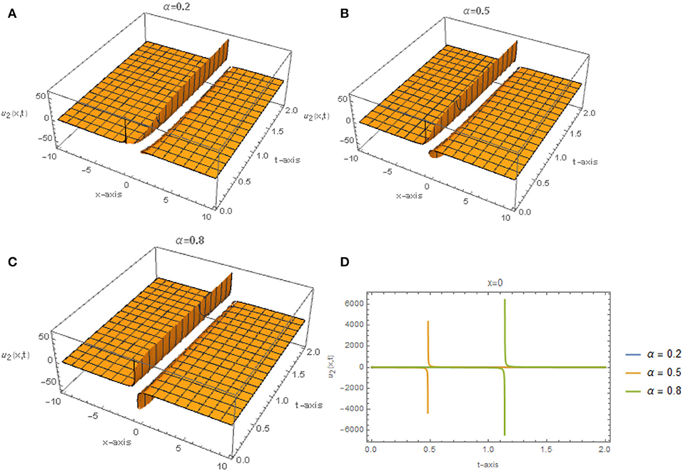
Figure 3. (A–D) The Solution u_2 (x,t) given by Eq. (50).

FIGURE 4

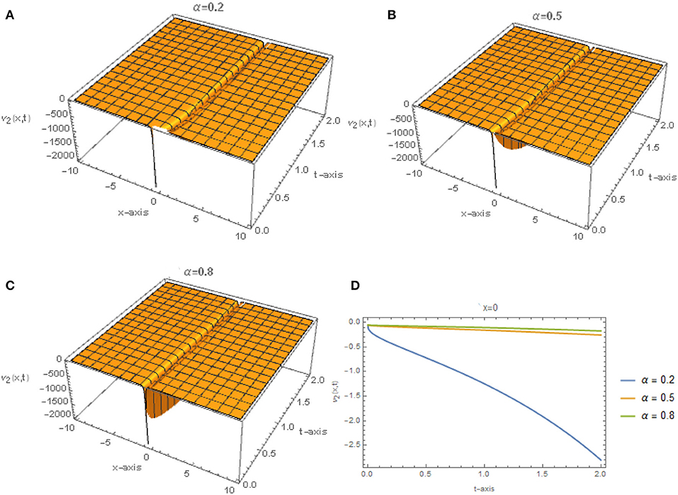
Figure 4. (A–D) The Solution v_2 (x,t) given by Eq. (50).

The Time-Fractional Wu-Zhang System of Equations

Let us consider the time-fractional Wu-Zhang system of equations

$\begin{array}{ll}\begin{array}{c}{D}_t^{\alpha }u+u{u}_x+v_x=0\\ D_t^{\alpha }v+{(uv)}_x+\frac{1}{3}{u}_{xxx}=0\end{array}\},t\ge 0,0<\alpha \le 1.& (70)\end{array}$

Now, applying under the traveling wave transformation of Eq. (6), Eq. (71) reduces to a non-linear ODE as

$\begin{array}{ll}\begin{array}{c}-c{U}^{\prime }+U{U}^{\prime }+V^{\prime }=0\\ -c{V}^{\prime }+{(UV)}^{\prime }+\frac{1}{3}{U}^{‴}=0\end{array}\}.& (71)\end{array}$

Integrating with respect to ξ of Eq. (71) and considering the integration constant is zero. Then Eq. (72) yields

$\begin{array}{ll}\begin{array}{c}-cU+\frac{1}{2}{U}^2+V=0\\ -cV+UV+\frac{1}{3}{U}^{″}=0\end{array}\},& (72)\end{array}$

Following the steps given in the last two sections we reach to m = 1 and n = 2. Consequently, the general solution will take the form

$\begin{array}{ll}\begin{array}{c}U(\xi )=a_0+a_{1}exp(-\phi (\xi ))\\ V(\xi )=b_0+b_{1}exp(-\phi (\xi ))+b_{2}exp(-2\phi (\xi ))\end{array}\},& (73)\end{array}$

where a₁ ≠ 0 and b₂ ≠ 0.

Put Eq. (74) into Eq. (73) along with Eq. (9), and we get a new system of algebraic equations that solve to

Set-1: $a_0=\frac{1}{3}\sqrt{3}r\pm \frac{1}{3}\sqrt{3(r^2-4pq)},a_1=\frac{2}{3}\sqrt{3}p,b_0=-\frac{2}{3}pq,b_1=-\frac{2}{3}pr,b_2=-{\frac{2}{3}p}^2$

$\text{and }c=\pm \frac{1}{3}\sqrt{3(r^2-4pq)},-4pq+r^2>0$.

Therefore, by substituting the values of Set-1 into Eq. (74) along with the Eq. (10) to Eq. (18), we generate the following traveling wave solutions for the time-fractional Wu-Zhang system of equations.

For p = 1:

$\begin{array}{ll}\begin{array}{c}{u}_1(x,t)=\frac{1}{3}\sqrt{3}r\pm \frac{1}{3}\sqrt{3(r^2-4q)}\\ -\frac{4}{3}\frac{\sqrt{3}q}{\sqrt{\Delta }tanh\left(\frac{1}{2}\sqrt{\Delta }(\xi +E)\right)+r}\\ v_1(x,t)=-\frac{2}{3}q+\frac{4}{3}\frac{rq}{\sqrt{\Delta }tanh\left(\frac{1}{2}\sqrt{\Delta }(\xi +E)\right)+r}\\ -\frac{8}{3}\frac{q^2}{{\left(\sqrt{\Delta }tanh\left(\frac{1}{2}\sqrt{\Delta }(\xi +E)\right)+r\right)}^2}\end{array}\},& (74)\end{array}$

$\begin{array}{ll}\begin{array}{c}{u}_2(x,t)=\frac{1}{3}\sqrt{3}r\pm \frac{1}{3}\sqrt{3\left(r^2-4q\right)}\\ -\frac{4}{3}\frac{\sqrt{3}q}{\sqrt{\Delta }coth\left(\frac{1}{2}\sqrt{\Delta }(\xi +E)\right)+r}\\ v_2(x,t)=-\frac{2}{3}q+\frac{4}{3}\frac{rq}{\sqrt{\Delta }coth\left(\frac{1}{2}\sqrt{\Delta }(\xi +E)\right)+r}\\ -\frac{8}{3}\frac{q^2}{{\left(coth\left(\frac{1}{2}\sqrt{\Delta }(\xi +E)\right)+r\right)}^2}\end{array}\},& (75)\end{array}$

$\begin{array}{ll}\begin{array}{c}{u}_3(x,t)=\frac{1}{3}\sqrt{3}r\pm \frac{1}{3}\sqrt{3\left(r^2-4q\right)}\\ +\frac{4}{3}\frac{\sqrt{3}q}{\sqrt{-\Delta }tan\left(\frac{1}{2}\sqrt{-\Delta }(\xi +E)\right)-r}\\ v_3(x,t)=-\frac{2}{3}q-\frac{4}{3}\frac{rq}{\sqrt{-\Delta }tan\left(\frac{1}{2}\sqrt{-\Delta }(\xi +E)\right)+r}\\ -\frac{8}{3}\frac{q^2}{{\left(\sqrt{-\Delta }tan\left(\frac{1}{2}\sqrt{-\Delta }(\xi +E)\right)-r\right)}^2}\end{array}\},& (76)\end{array}$

$\begin{array}{ll}\begin{array}{c}{u}_4(x,t)=\frac{1}{3}\sqrt{3}r\pm \frac{1}{3}\sqrt{3\left(r^2-4q\right)}\\ +\frac{4}{3}\frac{\sqrt{3}q}{\sqrt{-\Delta }cot\left(\frac{1}{2}\sqrt{-\Delta }(\xi +E)\right)-r}\\ v_4(x,t)=-\frac{2}{3}q-\frac{4}{3}\frac{rq}{\sqrt{-\Delta }cot\left(\frac{1}{2}\sqrt{-\Delta }(\xi +E)\right)+r}\\ -\frac{8}{3}\frac{q^2}{{\left(\sqrt{-\Delta }cot\left(\frac{1}{2}\sqrt{-\Delta }(\xi +E)\right)-r\right)}^2}\end{array}\},& (77)\end{array}$

$\begin{array}{ll}\begin{array}{c}{u}_5(x,t)=\frac{1}{3}\sqrt{3}r\pm \frac{1}{3}\sqrt{3\left(r^2-4q\right)}+\frac{2}{3}\frac{\sqrt{3}r}{e^{r(\xi +E)}-1}\\ v_5(x,t)=-\frac{2}{3}q-\frac{2}{3}\frac{r^2}{e^{r(\xi +E)}-1}-\frac{2}{3}\frac{r^2}{{(e^{r(\xi +E)}-1)}^2}\end{array}\},& (78)\end{array}$

and

$\begin{array}{ll}\begin{array}{c}{u}_6\left(x,t\right)=\frac{1}{3}\sqrt{3}r\pm \frac{1}{3}\sqrt{3(r^2-4q)}-\frac{1}{3}\frac{\sqrt{3}{r}^2(\xi +E)}{r(\xi +E)+2}\\ v_6(x,t)=-\frac{2}{3}q+\frac{1}{3}\frac{r^3(\xi +E)}{r(\xi +E)+2}-\frac{1}{6}{\left(\frac{r^2(\xi +E)}{r(\xi +E)+2}\right)}^2\end{array}\},& (79)\end{array}$

where, $\xi =x\mp \left(\frac{1}{3}\sqrt{3(r^2-4q)}\right)\frac{t^{\alpha }}{\alpha }$ and Δ = r² − 4q > 0.

For r = 0:

$\begin{array}{ll}\begin{array}{c}{u}_7\left(x,t\right)=\pm \frac{2}{3}\sqrt{-3pq}+\frac{2}{3}\frac{\sqrt{3pq}}{tan\left(\sqrt{pq}\left(\xi +E\right)\right)}\\ v_7\left(x,t\right)=-\frac{2}{3}pq-\frac{2}{3}{\left(\frac{\sqrt{pq}}{tan\left(\sqrt{pq}\left(\xi +E\right)\right)}\right)}^2\end{array}\},& (80)\end{array}$

$\begin{array}{ll}\begin{array}{c}{u}_8\left(x,t\right)=\pm \frac{2}{3}\sqrt{-3pq}-\frac{2}{3}\frac{\sqrt{3pq}}{cot\left(\sqrt{pq}\left(\xi +E\right)\right)}\\ v_8\left(x,t\right)=-\frac{2}{3}pq-\frac{2}{3}{\left(\frac{\sqrt{pq}}{cot\left(\sqrt{pq}\left(\xi +E\right)\right)}\right)}^2\end{array}\},& (81)\end{array}$

$\begin{array}{ll}\begin{array}{c}{u}_9\left(x,t\right)=\pm \frac{2}{3}\sqrt{-3pq}+\frac{2}{3}\frac{\sqrt{-3pq}}{tanh\left(\sqrt{-pq}\left(\xi +E\right)\right)}\\ v_9\left(x,t\right)=-\frac{2}{3}pq+\frac{2}{3}{\left(\frac{\sqrt{pq}}{tanh\left(\sqrt{-pq}\left(\xi +E\right)\right)}\right)}^2\end{array}\},& (82)\end{array}$

and

$\begin{array}{ll}\begin{array}{c}{u}_{10}\left(x,t\right)=\pm \frac{2}{3}\sqrt{-3pq}-\frac{2}{3}\frac{\sqrt{-3pq}}{coth\left(\sqrt{-pq}\left(\xi +E\right)\right)}\\ v_{10}\left(x,t\right)=-\frac{2}{3}pq+\frac{2}{3}{\left(\frac{\sqrt{pq}}{coth\left(\sqrt{-pq}\left(\xi +E\right)\right)}\right)}^2\end{array}\},& (83)\end{array}$

where, $\xi =x\mp \left(\frac{2}{3}\sqrt{-3pq}\right)\frac{t^{\alpha }}{\alpha },pq<0$.

For q = 0 and r = 0:

$\begin{array}{ll}\begin{array}{c}{u}_{11}(x,t)=\frac{2}{3}\frac{\sqrt{3}}{x+E}\\ v_{11}(x,t)=-{\frac{2}{3}\left(\frac{1}{x+E}\right)}^2\end{array}\}.& (84)\end{array}$

Set-2: $a_0=-\frac{1}{3}\sqrt{3}r\pm \frac{1}{3}\sqrt{3(r^2-4pq)},a_1=-\frac{2}{3}\sqrt{3}p,b_0=-\frac{2}{3}pq,b_1=-\frac{2}{3}pr,b_2=-{\frac{2}{3}p}^2$

$\text{and }c=\pm \frac{1}{3}\sqrt{3(r^2-4pq)},-4pq+r^2>0$.

Consequently, by substituting the values of Set-2 into Eq. (74) along with the Eq. (10) to Eq. (18), we generate the following traveling wave solutions for the time-fractional Wu-Zhang system of equations.

For p = 1:

$\begin{array}{ll}\begin{array}{c}{u}_{12}(x,t)=-\frac{1}{3}\sqrt{3}r\pm \frac{1}{3}\sqrt{3\left(r^2-4q\right)}\\ +\frac{4}{3}\frac{\sqrt{3}q}{\sqrt{\Delta }tanh\left(\frac{1}{2}\sqrt{\Delta }(\xi +E)\right)+r}\\ v_{12}(x,t)=-\frac{2}{3}q+\frac{4}{3}\frac{rq}{\sqrt{\Delta }tanh\left(\frac{1}{2}\sqrt{\Delta }(\xi +E)\right)+r}\\ -\frac{8}{3}\frac{q^2}{{\left(\sqrt{\Delta }tanh\left(\frac{1}{2}\sqrt{\Delta }(\xi +E)\right)+r\right)}^2}\end{array}\},& (85)\end{array}$

$\begin{array}{ll}\begin{array}{c}{u}_{13}(x,t)=-\frac{1}{3}\sqrt{3}r\pm \frac{1}{3}\sqrt{3\left(r^2-4q\right)}\\ +\frac{4}{3}\frac{\sqrt{3}q}{\sqrt{\Delta }coth\left(\frac{1}{2}\sqrt{\Delta }(\xi +E)\right)+r}\\ v_{13}(x,t)=-\frac{2}{3}q+\frac{4}{3}\frac{rq}{\sqrt{\Delta }coth\left(\frac{1}{2}\sqrt{\Delta }(\xi +E)\right)+r}\\ -\frac{8}{3}\frac{q^2}{{\left(\sqrt{\Delta }coth\left(\frac{1}{2}\sqrt{\Delta }(\xi +E)\right)+r\right)}^2}\end{array}\}& (86)\end{array}$

$\begin{array}{ll}\begin{array}{c}{u}_{14}(x,t)=-\frac{1}{3}\sqrt{3}r\pm \frac{1}{3}\sqrt{3\left(r^2-4q\right)}\\ -\frac{4}{3}\frac{\sqrt{3}q}{\sqrt{-\Delta }tan\left(\frac{1}{2}\sqrt{-\Delta }(\xi +E)\right)-r}\\ v_{14}(x,t)=-\frac{2}{3}q+\frac{4}{3}\frac{rq}{\sqrt{-\Delta }tan\left(\frac{1}{2}\sqrt{-\Delta }(\xi +E)\right)+r}\\ -\frac{8}{3}\frac{q^2}{{\left(\sqrt{-\Delta }tan\left(\frac{1}{2}\sqrt{-\Delta }(\xi +E)\right)-r\right)}^2}\end{array}\},& (87)\end{array}$

$\begin{array}{ll}\begin{array}{c}{u}_{15}(x,t)=-\frac{1}{3}\sqrt{3}r\pm \frac{1}{3}\sqrt{3\left(r^2-4q\right)}\\ -\frac{4}{3}\frac{\sqrt{3}q}{\sqrt{-\Delta }cot\left(\frac{1}{2}\sqrt{-\Delta }(\xi +E)\right)-r}\\ v_{15}(x,t)=-\frac{2}{3}q-\frac{4}{3}\frac{rq}{\sqrt{-\Delta }cot\left(\frac{1}{2}\sqrt{-\Delta }(\xi +E)\right)+r}\\ -\frac{8}{3}\frac{q^2}{{\left(\sqrt{-\Delta }cot\left(\frac{1}{2}\sqrt{-\Delta }(\xi +E)\right)-r\right)}^2}\end{array}\},& (88)\end{array}$

$\begin{array}{ll}\begin{array}{c}{u}_{16}(x,t)=-\frac{1}{3}\sqrt{3}r\pm \frac{1}{3}\sqrt{3\left(r^2-4q\right)}-\frac{2}{3}\frac{\sqrt{3}r}{e^{r(\xi +E)}-1}\\ v_{16}(x,t)=-\frac{2}{3}q-\frac{2}{3}\frac{r^2}{e^{r(\xi +E)}-1}-\frac{2}{3}\frac{r^2}{{(e^{r(\xi +E)}-1)}^2}\end{array}\},& (89)\end{array}$

and

$\begin{array}{ll}\begin{array}{c}{u}_{17}(x,t)=-\frac{1}{3}\sqrt{3}r\pm \frac{1}{3}\sqrt{3\left(r^2-4q\right)}+\frac{1}{3}\frac{\sqrt{3}{r}^2(\xi +E)}{r(\xi +E)+2}\\ v_{17}(x,t)=-\frac{2}{3}q+\frac{1}{3}\frac{r^3(\xi +E)}{r(\xi +E)+2}-\frac{1}{6}{\left(\frac{r^2(\xi +E)}{r(\xi +E)+2}\right)}^2\end{array}\},& (90)\end{array}$

where, $\xi =x\mp \left(\frac{1}{3}\sqrt{3(r^2-4q)}\right)\frac{t^{\alpha }}{\alpha }$ and Δ = r² − 4q > 0.

For r = 0:

$\begin{array}{ll}\begin{array}{c}{u}_{18}(x,t)=\pm \frac{2}{3}\sqrt{-3pq}-\frac{2}{3}\frac{\sqrt{3pq}}{\tan ((\xi +E))}\\ v_{18}(x,t)=-\frac{2}{3}pq-\frac{2}{3}{\left(\frac{\sqrt{pq}}{tan(\sqrt{pq}(\xi +E))}\right)}^2\end{array}\},& (91)\end{array}$

$\begin{array}{ll}\begin{array}{c}{u}_{19}(x,t)=\pm \frac{2}{3}\sqrt{-3pq}+\frac{2}{3}\frac{\sqrt{3pq}}{\cos \left(\sqrt{pq}(\xi +E)\right)}\\ v_{19}(x,t)=-\frac{2}{3}pq-\frac{2}{3}{\left(\frac{\sqrt{pq}}{cot(\sqrt{pq}(\xi +E))}\right)}^2\end{array}\},& (92)\end{array}$

$\begin{array}{ll}\begin{array}{c}{u}_{20}(x,t)=\pm \frac{2}{3}\sqrt{-3pq}-\frac{2}{3}\frac{\sqrt{-3pq}}{\tanh \left(\sqrt{-pq}(\xi +E)\right)}\\ v_{20}(x,t)=-\frac{2}{3}pq+\frac{2}{3}{\left(\frac{\sqrt{-pq}}{tanh(\sqrt{pq}(\xi +E))}\right)}^2\end{array}\},& (93)\end{array}$

and

$\begin{array}{ll}\begin{array}{c}{u}_{21}(x,t)=\pm \frac{2}{3}\sqrt{-3pq}+\frac{2}{3}\frac{\sqrt{-3pq}}{\coth \left(\sqrt{-pq}(\xi +E)\right)}\\ v_{21}(x,t)=-\frac{2}{3}pq+\frac{2}{3}{\left(\frac{\sqrt{pq}}{coth(\sqrt{-pq}(\xi +E))}\right)}^2\end{array}\},& (94)\end{array}$

where, $\xi =x\mp \left(\frac{2}{3}\sqrt{-3pq}\right)\frac{t^{\alpha }}{\alpha },pq<0$.

For q = 0 and r = 0:

$\begin{array}{ll}\begin{array}{c}{u}_{22}(x,t)=\frac{2}{3}\frac{\sqrt{3}}{x+E}\\ v_{22}(x,t)=-{\frac{2}{3}\left(\frac{1}{x+E}\right)}^2\end{array}\}.& (95)\end{array}$

Figures 5, 6 represent the solutions given by Eq. (79) for different values of α when r = 3, q = 2 and E = 0.

FIGURE 5

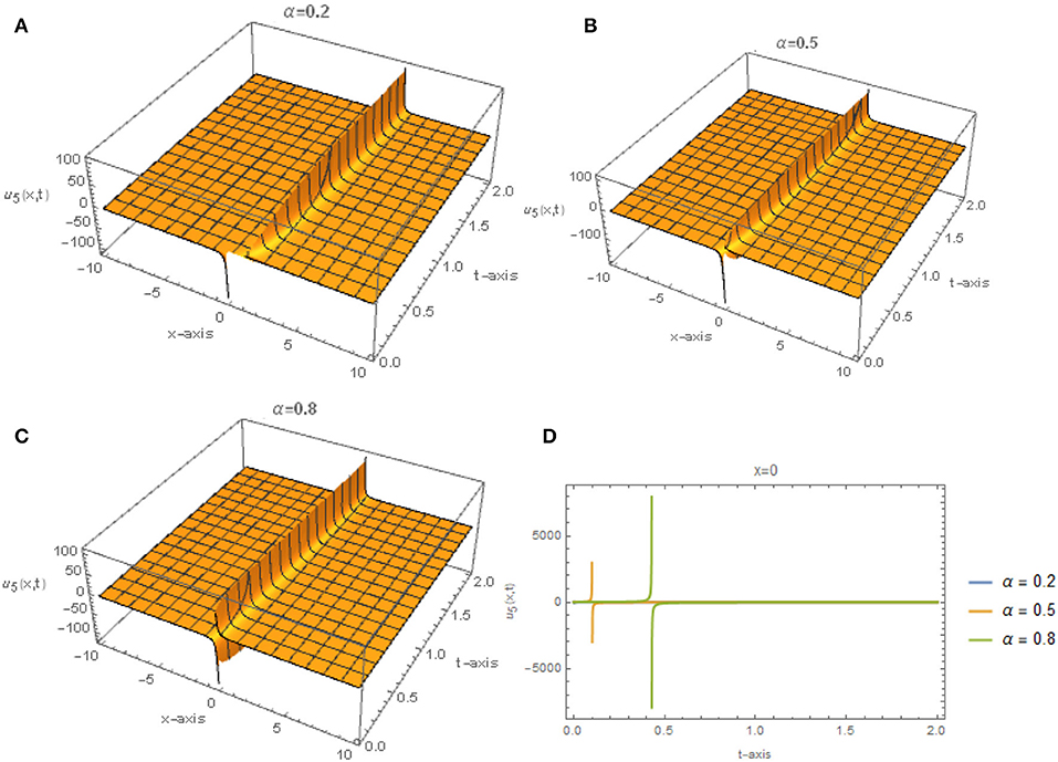
Figure 5. (A–D) The Solution u_5 (x,t) given by Eq. (79).

FIGURE 6

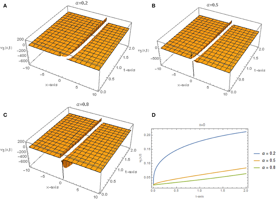
Figure 6. (A–D) The Solution v_5 (x,t) given by Eq. (79).

Conclusion

This research successfully applied the generalized exp(−φ(ξ))-expansion method combined with the complex fractional transformation and conformable derivative to exactly solve a special class of time-fractional WBK equations in shallow water, such as the time-fractional ALW equations, the time-fractional variant-Boussinesq equations, and the time fractional Wu-Zhang system of equations. Afterwards, a sequence of new analytical wave solutions for these models were established. Finally, some 3D and 2D plots were added for some of the gained solutions for every model to illustrate the effect of the parameter α on the behaviors of these solutions. In conclusion, we found that the method mentioned here—with the aid of symbolic computations—is aspiring and efficient, and it is a superior mathematical construction with which to deal with the NPDEs.

Data Availability Statement

The original contributions presented in the study are included in the article/supplementary materials, further inquiries can be directed to the corresponding author/s.

Author Contributions

All authors listed have made a substantial, direct and intellectual contribution to the work, and approved it for publication.

Conflict of Interest

The authors declare that the research was conducted in the absence of any commercial or financial relationships that could be construed as a potential conflict of interest.

The reviewer MB declared a past co-authorship with one of the authors DB to the handling editor.

References

1. Guo S, Mei LQ, Li Y, Sun YF. The improved fractional sub-equation method and its applications to the space–time-fractional differential equations in fluid mechanics. Phys Lett A. (2012) 376:407–11. doi: 10.1016/j.physleta.2011.10.056

CrossRef Full Text | Google Scholar

2. El-Borai MM, El-Sayed WG, Al-Masroub RM. Exact solution for time-fractional coupled Whitham-Broer-Kaup equations via exp-function method. Int Res J Eng Tech. (2015) 2:307–15. doi: 10.1016/j.chaos.2004.09.017

CrossRef Full Text | Google Scholar

3. Ghanbari B, Osman MS, Baleanu D. Generalized exponential rational function method for extended Zakharov–Kuzetsov equation with conformable derivative. Modern Phys Lett A. (2019) 34:1950155. doi: 10.1142/S0217732319501554

CrossRef Full Text | Google Scholar

4. Guner O, Atik H, Kayyrzhanovich AA. New exact solution for space–time-fractional differential equations via G′/G-expansion method. Optik. (2017) 130:696–701. doi: 10.1016/j.ijleo.2016.10.116

CrossRef Full Text | Google Scholar

5. Liu JG, Osman MS, Zhu WH, Zhou L, Ai GP. Different complex wave structures described by the hirota equation with variable coefficients in inhomogeneous optical fibers. Appl Phys B. (2019) 125:175. doi: 10.1007/s00340-019-7287-8

PubMed Abstract | CrossRef Full Text | Google Scholar

6. Ding Y, Osman MS, Wazwaz AM. Abundant complex wave solutions for the nonautonomous Fokas–Lenells equation in presence of perturbation terms. Optik. (2019) 181:503–13. doi: 10.1016/j.ijleo.2018.12.064

CrossRef Full Text | Google Scholar

7. Liu JG, Osman MS, Wazwaz AM. A variety of nonautonomous complex wave solutions for the (2+ 1)-dimensional nonlinear Schrödinger equation with variable coefficients in nonlinear optical fibers. Optik. (2019) 180:917–23. doi: 10.1016/j.ijleo.2018.12.002

CrossRef Full Text | Google Scholar

8. Manafian J, Lakestani M. Abundant soliton solutions for the Kundu–Eckhaus equation via tan(Φ(ξ)/2)-expansion method. Optik. (2016) 127:5543–51. doi: 10.1016/j.ijleo.2016.03.041

CrossRef Full Text | Google Scholar

9. Ray SS. New analytical exact solutions of time-fractional KdV–KZK equation by Kudryashov methods. Chinese Phys B. (2016) 25:040204. doi: 10.1088/1674-1056/25/4/040204

CrossRef Full Text | Google Scholar

10. Hosseini K, Mayeli P, Kumar D. New exact solutions of the coupled sine-Gordon equation in nonlinear optics using the modified Kudryashov method. J Modern Optics. (2018) 65:361–4. doi: 10.1080/09500340.2017.1380857

CrossRef Full Text | Google Scholar

11. Rezazadeh H, Mirhosseini-Alizamini SM, Eslami M, Rezazadeh M, Mirzazadeh Abbagari MS. New optical solitons of conformable fractional Schrödinger-Hirota equation. Optik. (2018) 172:545–53. doi: 10.1016/j.ijleo.2018.06.111

CrossRef Full Text | Google Scholar

12. Kumar D, Kaplan M. New analytical solutions of (2+1)-dimensional conformable time-fractional Zoomeron equation via two distinct techniques. Chinese J Phys. (2018) 56:2173–85. doi: 10.1016/j.cjph.2018.09.013

CrossRef Full Text | Google Scholar

13. Inc M, Yusuf A, Aliyu AI, Baleanu D. Soliton structures to some time-fractional nonlinear differential equations with conformable derivative. Opt Quant Elect. (2018) 50:20. doi: 10.1007/s11082-018-1459-3

CrossRef Full Text | Google Scholar

14. Kumar D, Hosseini K, Samadani F. The sine-Gordon expansion method to look for the traveling wave solutions of the Tzitzeica type equations in nonlinear optics. Optik. (2017) 149:439–46. doi: 10.1016/j.ijleo.2017.09.066

CrossRef Full Text | Google Scholar

15. Ali KK, Wazwaz AM, Osman MS. Optical soliton solutions to the generalized nonautonomous nonlinear Schrödinger equations in optical fibers via the sine-Gordon expansion method. Optik. (2019) 208:164132. doi: 10.1016/j.ijleo.2019.164132

CrossRef Full Text | Google Scholar

16. Ali KK, Osman MS, Abdel-Aty M. New optical solitary wave solutions of Fokas-Lenells equation in optical fiber via Sine-Gordon expansion method. Alexand Eng J. (2020). doi: 10.1016/j.aej.2020.01.037

CrossRef Full Text | Google Scholar

17. Osman MS, Lu D, Khater MM. A study of optical wave propagation in the nonautonomous Schrödinger-Hirota equation with power-law nonlinearity. Res Phys. (2019) 13:102157. doi: 10.1016/j.rinp.2019.102157

CrossRef Full Text | Google Scholar

18. Osman MS. New analytical study of water waves described by coupled fractional variant Boussinesq equation in fluid dynamics. Pramana. (2019) 93:26. doi: 10.1007/s12043-019-1785-4

CrossRef Full Text | Google Scholar

19. Javid A, Raza N, Osman MS. Multi-solitons of thermophoretic motion equation depicting the wrinkle propagation in substrate-supported graphene sheets. Commun Theor Phys. (2019) 71:362. doi: 10.1088/0253-6102/71/4/362

CrossRef Full Text | Google Scholar

20. Osman MS. Nonlinear interaction of solitary waves described by multi-rational wave solutions of the (2+1)-dimensional Kadomtsev–Petviashvili equation with variable coefficients. Nonlinear Dynamics. (2017) 87:1209–16. doi: 10.1007/s11071-016-3110-9

CrossRef Full Text | Google Scholar

21. Ray SS. A novel method for travelling wave solutions of fractional Whitham-Broer-Kaup, fractional modified Boussinesq and fractional approximate long wave equations in shallow water. Math Methods Appl Sci. (2015) 38:1352–68. doi: 10.1002/mma.3151

CrossRef Full Text | Google Scholar

22. Ping Z. New exact solutions to breaking solution equations and Whitham–Broer–Kaup equation. Appl. Math. Comput. (2010) 217:1688–96. doi: 10.1016/j.amc.2009.09.062

CrossRef Full Text | Google Scholar

23. Kupershmidt BA. Mathematics of dispersive water waves. Commun Math Phys. (1985) 99:51–73. doi: 10.1007/BF01466593

CrossRef Full Text | Google Scholar

24. Guo S, Liquan M. Exact solutions of space–time-fractional variant Boussinesq equations. Adv Sci Lett. (2012) 10:700–2. doi: 10.1166/asl.2012.3388

CrossRef Full Text | Google Scholar

25. El-Borai MM, El-Sayed WG, Al-Masroub RM. Exact solution for time-fractional coupled Whitham-Broer-Kaup equations via exp-function method. Int. Res. J. Eng. Tech. (2015) 2:307–15.

Google Scholar

26. Yan L. New travelling wave solutions for coupled fractional variant Boussinesq equation and approximate long water wave equation. Int. J. Numer. Methods Heat Fluid Flow. (2015) 25:33–40. doi: 10.1108/HFF-04-2013-0126

CrossRef Full Text | Google Scholar

27. Eslami M, Rezazadeh H. The first integral method for Wu-Zhang system with conformable time-fractional derivative. Calcolo. (2016) 53:475–85. doi: 10.1007/s10092-015-0158-8

CrossRef Full Text | Google Scholar

28. Whitham GB. Variational methods and applications to water waves. Proc R Soc Lond Series A. (1967) 299:6–25. doi: 10.1098/rspa.1967.0119

CrossRef Full Text | Google Scholar

29. Broer LJF. Approximate equations for long water waves. Appl Sci Res. (1975) 31:377–95. doi: 10.1007/BF00418048

CrossRef Full Text | Google Scholar

30. Kaup DJ. A higher-order water-wave equation and the method for solving it. Prog Theor Phys. (1975) 54:396–408. doi: 10.1143/PTP.54.396

CrossRef Full Text | Google Scholar

31. Gao H, Tianzhou X, Shaojie Y, Gangwei W. Analytical study of solitons for the variant Boussinesq equations. Nonlinear Dyn. (2017) 88:1139–46. doi: 10.1007/s11071-016-3300-5

CrossRef Full Text | Google Scholar

32. Hosseini K, Ansari R, Gholamin P. Exact solutions of some nonlinear systems of partial differential equations by using the first integral method. J Math Anal App. (2012) 387:807–14. doi: 10.1016/j.jmaa.2011.09.044

CrossRef Full Text | Google Scholar

33. Zheng X, Yong C, Hongqing Z. Generalized extended tanh-function method and its application to (1+1)-dimensional dispersive long wave equation. Phys Lett A. (2003) 311:145–57. doi: 10.1016/S0375-9601(03)00451-1

CrossRef Full Text | Google Scholar

34. Chen Y, Qi W. A new general algebraic method with symbolic computation to construct new travelling wave solution for the (1+1)-dimensional dispersive long wave equation. Appl Math Comput. (2005) 168:1189–204. doi: 10.1016/j.amc.2004.10.012

CrossRef Full Text | Google Scholar

35. Elgarayhi A. New solitons and periodic wave solutions for the dispersive long wave equations. Phys A. (2006) 361:416–28. doi: 10.1016/j.physa.2005.05.103

CrossRef Full Text | Google Scholar

36. Lu D, Chen Y, Muhammad A. Traveling wave solutions of space–time-fractional generalized fifth-order KdV equation. Adv Math Phys. (2017) 12:1–6. doi: 10.1155/2017/6743276

CrossRef Full Text | Google Scholar

37. Khalil R, Al Horani M, Yousef A, Sababheh M. A new definition of fractional derivative. J Comput Appl Math. (2014) 264:65–70. doi: 10.1016/j.cam.2014.01.002

CrossRef Full Text | Google Scholar

38. Abdeljawad T. On conformable fractional calculus. J Comput Appl Math. (2015) 279:57–66. doi: 10.1016/j.cam.2014.10.016

CrossRef Full Text | Google Scholar

39. Atangana A, Baleanu D, Alsaedi A. New properties of conformable derivative. Open Math. (2015) 13:889–98. doi: 10.1515/math-2015-0081

CrossRef Full Text | Google Scholar

40. Çenesiz Y, Baleanu D, Kurt A, Tasbozan O. New exact solutions of Burgers' type equations with conformable derivative. Waves Rand Compl Media. (2017) 27:103–16. doi: 10.1080/17455030.2016.1205237

CrossRef Full Text | Google Scholar

41. Zhou HW, Yang S, Zhang SQ. Conformable derivative approach to anomalous diffusion. Physica A. (2018) 491:1001–13. doi: 10.1016/j.physa.2017.09.101

CrossRef Full Text | Google Scholar