 Zhiyong Huang1
95% of researchers rate our articles as excellent or good
Learn more about the work of our research integrity team to safeguard the quality of each article we publish.
Find out more
ORIGINAL RESEARCH article
Front. Mater. , 30 March 2022
Sec. Structural Materials
Volume 9 - 2022 | https://doi.org/10.3389/fmats.2022.850694
This article is part of the Research Topic 2022 Retrospective: Structural Materials View all 5 articles
The three-dimensional ground-penetrating radar system is an effective method to detect road void disease. Ground penetrating radar image interpretation has the characteristics of multi-solution, long interpretation period, and high professional requirements of processors. In recent years, researchers have put forward solutions for automatic interpretation of ground-penetrating radar images, including automatic detection algorithm for subgrade diseases based on support vector machines, etc., but there are still some shortcomings such as training models with a large amount of data or setting parameters. In this article, a three-dimensional ground-penetrating radar void signal recognition algorithm based on the digital image is proposed, and the algorithm uses digital images to characterize radar signals. With the help of digital image processing methods, the images are processed by binarization, corrosion, expansion, connected area inspection, fine length index inspection, and three-dimensional matching inspection, so as to identify and determine the void signals and extract the void area volume index. The algorithm has been verified by laboratory tests and engineering projects, and the results show that the void identification algorithm can accurately identify the void area position; the error level between the measured values and the measured values of length, width, buried depth, and area is between 2.2 and 17.3%, and the error is generally within the engineering acceptance range. The volume index calculated by the algorithm has a certain engineering application value; compared with the support vector machine, the regressive convolution neural network, and other recognition methods, it has the advantage of not needing a large amount of data to train or modify parameters.
Internal void of the road structure refers to the void formed in the structural layer due to erosion of subgrade backfill soil or base course and sinking of the substructure layer. Under the continuous action of formation conditions, voids that are not detected and treated in time may develop and expand further, causing pavement subsidence or collapse accidents and threatening driving safety (Syaifuddin, 2014; Liu et al., 2021; Zou et al., 2021). For roads or areas with void risk, it is necessary to carry out void investigation and detection, give early warning, and treat void diseases. Ground-penetrating radar (GPR) detection technology is one of the representative technologies of road nondestructive testing technology. It mainly obtains the relevant information of the detected objects by analyzing the propagation of electromagnetic waves inside the detected objects, including the information of road internal diseases such as voids. Compared with the traditional core drilling technology, it has the advantages of rapidity and nondestructiveness (Yan et al., 2011; Liu et al., 2014; Klotzsche et al., 2019; Wang et al., 2020a).
Among the ground-penetrating radars with various mechanisms, the two-dimensional ground-penetrating radar can only collect one vertical section data at a time when detecting pavement engineering diseases, which can only make qualitative analysis of diseases and is easy to misjudge and miss diseases. Three-dimensional ground-penetrating radar adopts multi-antenna setting and multi-section data combination judgment, which has the advantages of full coverage, high accuracy of disease judgment, and quantitative analysis of diseases (Allroggen and Tronicke, 2020; Domenzain et al., 2020; Tosti and Ferrante, 2020). In this article, 3D GPR images are used to carry out automatic recognition of void images.
Because GPR image interpretation has multiple solutions, it is impossible to infer the internal conditions of the road structure only according to radar images, and it is necessary to exclude some interpretations by combining radar theoretical basis, engineering experience, and other related knowledge and experience, so as to obtain correct interpretation of radar images (Fenning et al., 2003; Leng and Al-Qadi, 2014; Huai et al., 2019; Kumlu, 2021). The manual interpretation process has long-period, low-efficiency, and high-professional requirements of processing personnel. At present, radar image interpretation is a difficult point in the application of GPR disease detection, and it is also one of the reasons that limit the development of GPR application (Song and Larkin, 2016; Cha et al., 2017).
In recent years, with the rapid development of automatic signal-processing algorithms, researchers have proposed many radar signal-processing algorithms to reduce the difficulty of image interpretation, and even achieve the purpose of automatic recognition. Zhou et al. (2013) proposed an automatic detection algorithm for subgrade diseases based on support vector machine (SVM). The algorithm uses objective information such as the thickness of expressway subgrade, and the amplitude of the reflected signal at the layer interface will change. Combined with GPR clutter suppression, layer interface detection and smoothing, region of interest (ROI) extraction, feature extraction, and pattern recognition technology, the detection results of this algorithm are compared with the ground truth database constructed by combining expert experience and drilling coring samples, and the coincidence degree is as high as 92.7%.
Sha A used the ground-penetrating radar profile to train the neural network based on cascade convolution (Sha et al., 2018),. The cascade convolution neural network system is composed of two convolution neural networks, which are used to identify low-resolution and high-resolution GPR images. After training the model with 46,080 images, the author uses the model to process 3,840 test data and detects vertical cracks, uneven settlement, and interlayer voids, with an accuracy rate of 94.5%.
A vision measurement system was developed to track the full field deformation of the specimen, and a four eye vision system was constructed to determine the deformation of the concrete column. The deformation was compared with the deformation measured by laser using image and point cloud stitching algorithm. The results showed that the hysteretic curves of all specimens were non-extrusion hysteretic curves, the ductility coefficient was large, and the equivalent viscous damping coefficient was between 0.462 and 0.975 (Tang et al., 2022). In order to obtain the target information of bud cutting robot operation, an improved deep learning algorithm was adopted to quickly and accurately identify banana fruit, inflorescence axis, and flower bud. Therefore, the edge detection algorithm and geometric calculation were used to determine the cutting point on the inflorescence axis. A modified YOLOv3 model based on clustering optimization was proposed, and the model illustrated the influence of the headlamp and backlight on the model (Wu et al., 2021). A noncontact 3D deformation measurement method based on binocular vision was proposed. The method was applied to the deformation and strain test of a concrete-filled steel tubular column. Based on the proposed image processing algorithm and the principle of three-dimensional deformation measurement, a circle-fitting algorithm based on the least square method was proposed and applied to the binocular vision system for static and dynamic acquisition of three-dimensional deformation data of concrete-filled steel tubular columns (Tang et al., 2018).
At present, the accuracy of radar signal-processing algorithms is over 90%; however, the deficiency is that the support vector machine (SVM) algorithm needs a lot of data to calculate and set up the SVM mapping, and the algorithm based on the cascade convolution neural network needs a lot of data to train the model under the same working condition. The generalization ability of the two algorithms is insufficient, so it is necessary to re-carry out relevant experiments to correct the model when solving the problems under different working conditions. In this article, a void recognition algorithm based on digital image processing method is proposed. The algorithm uses digital images to characterize radar signals. With the help of digital image processing methods, the images are processed by binarization, corrosion, expansion, connected area inspection, thin length index inspection, and three-dimensional matching inspection, so as to identify void diseases and determine void area volume index. The model does not need a lot of data training or parameter correction.
The basic detection principle of three-dimensional ground-penetrating radar is to send high-frequency electromagnetic waves in the form of pulses to the ground. During the propagation of electromagnetic waves in underground media, when they encounter underground targets with electrical differences, the electromagnetic waves will be reflected (Saarenketo et al., 2014; Solla et al., 2014; Tong et al., 2017).
The reflection coefficient and the reflected signal level can generally be calculated by the following formula:
where
There are obvious differences in relative dielectric constants between void fillers and road building materials. The interior of the void is generally air with a relative dielectric constant of 1, and the relative dielectric constant of road materials was generally between 3 and 10. The electromagnetic wave emitted by 3D GPR will be reflected at the interface between the void and road material (Sarkar et al., 2019; Wang et al., 2020b).
After receiving the reflected electromagnetic wave signal, GPR draws a radar gray image according to the propagation time and amplitude of the signal. Manual identification of void signals is mainly based on the existence of a strong solid line signal with black sides (side lobe) and white middle (main lobe) on the radar longitudinal section map, and the existence of the white highlight area block signal differs from the surrounding area on the radar plan map at the corresponding position (Giertzuch et al., 2020).
The steps of void recognition algorithm based on the digital image processing method are shown in the following Figure 1.
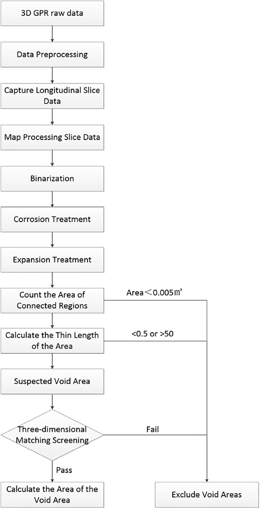
FIGURE 1. Steps of void recognition algorithm based on the digital image processing method.
In this article, a three-dimensional ground-penetrating radar system consisting of GeoScope™ MKIV radar host and DXG series multichannel ground-coupled antenna array is used. The antenna emits electromagnetic waves in a stepped frequency mode, with a frequency range of 200MHz–3 GHz and a width of 1.5 m. There are 11 transmitting antennas and 10 receiving antennas, and 20 pairs of antennas are formed by pairing and combining.
Sampling parameters are set as follows: the sampling interval is 2.5 cm, the time window is set to 50ns, and the standing wave time is set to 3 µs Under these parameters, the lateral spacing of the collected data matrix is 0.071 m, the driving direction spacing is 0.025 m, and the vertical spacing is about 0.0055 m (related to the dielectric characteristics, the time interval is 0.122 ns). Radar raw data are processed by 3dr-Examiner software, and the original data are frequency-domain data. The processing software converts frequency domain data into time domain data
where
Conventional data processing steps such as noise suppression, background removal, and automatic gain are needed for the data. The principle and detailed analysis of each step can be consulted in the article by Tang (2020). After the data are processed, a regular three-dimensional data lattice is formed.
In the process of data processing, three-dimensional data lattice can intercept two-dimensional lattice data by horizontal section, longitudinal section, and cross section and map radar signal data into 256 (0–255) intervals by using the image data method and assign an integer value to each interval, which corresponds to 256 Gy levels from white to black and draw a radar gray image. At the same time, in order to avoid the amplitude of individual radar signals being too large or too small, which leads to the overall black or white image representation and unrepresentativeness, 5% quantile value and 95% quantile value are selected as the upper and lower limits of mapping, and the conversion formula is shown in the following formula.
where
The radar longitudinal section obtained by data mapping is shown in Figure 2.
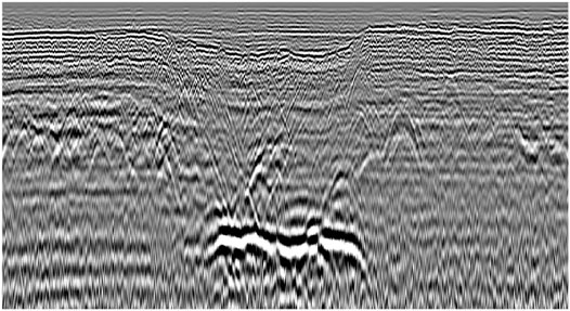
FIGURE 2. Longitudinal section of three-dimensional ground-penetrating radar.
The longitudinal section gray image drawn by radar signal amplitude is processed by the digital image processing method to determine the suspected void area. The processing steps are as follows:
The first step is to binary the longitudinal section diagram. The binarization method is to set the fifth% quantile of radar signal amplitude
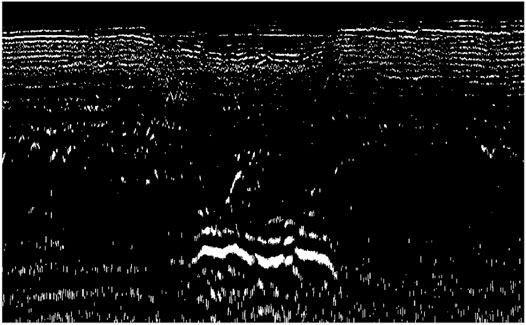
FIGURE 3. Binarization image (black corresponds to "0," and white corresponds to "1").
Step 2. : Etching the binary image. The etching treatment method is to etch the binary image A by using set B and a "1" matrix of 3 × 3. The corrosion process is made on A, and the process is as follows:
1) scanning each pixel of an image A with a structural element B;
2) make "AND" operation with structural elements and binary images covered by them;
3) if both are 1, the pixel of the resulting image is 1. Otherwise, it is 0.
Corrosion processing is a binary numerical image processing method, which can eliminate noise and weak connections in digital images, segment independent image elements, and find out obvious maximum areas in images. The main function of the binary longitudinal section diagram of corrosion treatment is to connect the whole area based on the empty internal air. Its reflection is strong, which can generally form a connected high-intensity reflected signal area and is not easy to be eliminated by corrosion treatment. The random noise, which is easy to be eliminated, and the interference signal with weak reflection intensity in the corrosion treatment image are adopted, and the processed image is shown in the following Figure 4.
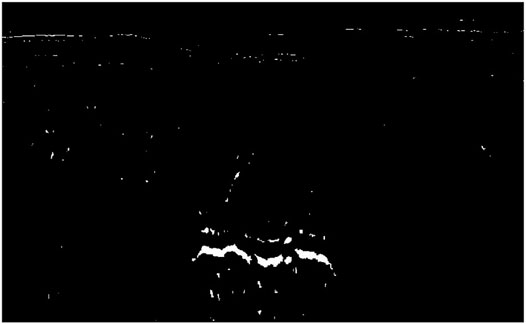
FIGURE 4. Binary image after etching treatment.
Step 3. : Dilate the binary image. Expansion treatment is the inverse process of corrosion treatment. Similar to corrosion treatment, expansion treatment uses set B and a "1″ matrix of 3 × 3 to process the binary image A after corrosion treatment. The process is as follows:
1) scanning each pixel of an image A with a structural element B;
2) using structural elements and their binary images to do "OR" operation;
3) if both are "0″, the pixel of the resulting image is "0". Otherwise, it is "1".
The main function of the binary longitudinal section image of expansion processing is to restore the corroded part of the image, so that the subsequent area statistics are accurate. The expansion processing also adopts the “1″ matrix of 3 × 3, and the processed image is shown in Figure 5.
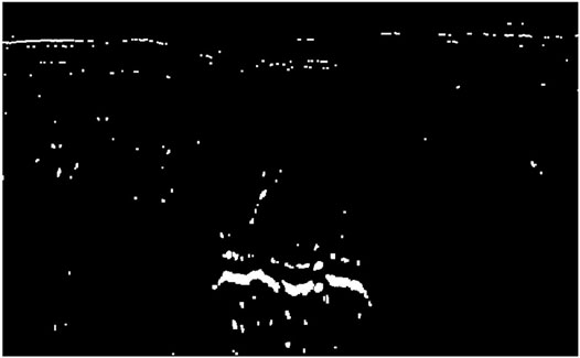
FIGURE 5. Binary image after dilation processing.
Step 4: Check and process the connected area.Region connectivity is an extended concept based on the concept of pixel adjacency. There are two criteria for judging pixel adjacency, one is 4-adjacency, and the other is 8-adjacency. A collection of pixels adjacent to each other is called a region. Connectivity means that there is at least one sequence of points
where

FIGURE 6. Binary image after connected region area check processing.
Step 5: Calculate the thin length of the area and screen the suspected void area. The slender length is calculated using the distance ratio represented by the largest pixel of the horizontal projection and vertical projection of the region, as shown in .
where
where
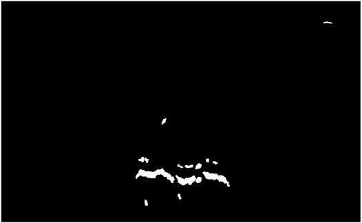
FIGURE 7. Binary image after fine length check processing of the connected region.
The lateral distance between adjacent channels of the 3D GPR antenna is 0.075 m. Considering the structural stability, the road structure changes slowly in a natural state. Under the distance of 0.075 m, the change range of adjacent longitudinal sections in the void area is small, and there is a certain overlapping area in the image. In the three-dimensional matching test of the void region, it is required that there is a certain proportion of suspected void region signals at the same position of adjacent longitudinal sections before judging the region as void signal. The inspection steps are as follows:
1) separate independently connected suspected void areas;
2) extract the same coordinate areas of adjacent longitudinal sections and check the proportion of suspected void areas in the extracted areas;
3) if the proportion of void areas in adjacent longitudinal section extraction areas is greater than 50%, it will pass the inspection; otherwise, it will not pass the inspection.
Check the void area of the adjacent longitudinal section map of 3D ground-penetrating radar data, and the test results are shown in Figure 8.
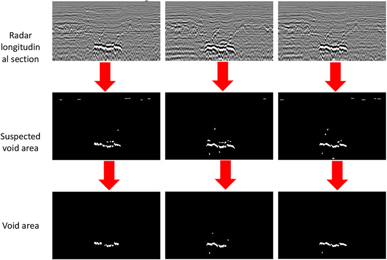
FIGURE 8. Determination of the suspected void area in the adjacent longitudinal section diagram.
After the three-dimensional matching test, it is confirmed that the main void area in the detection area is a large flat void at a depth of 2 m, with a length of 7 m, a width of 0.225 m, a height of 0.12 m, and a volume of about 0.189 m. Sporadic voids with small volume are distributed around the void area.
In order to verify the accuracy of the feasibility of the void recognition algorithm, a test site was selected, and a polystyrene void module was placed inside the test site to simulate the void environment inside the road. The three-dimensional ground-penetrating radar was used to scan the test field area, and the void recognition algorithm was used to process the scanned data and identify the void modules. According to the recognition results and the actual conditions inside the test area, the detection accuracy was compared. The embedding position and depth measurement site of the emptied module were shown in Figure 9.
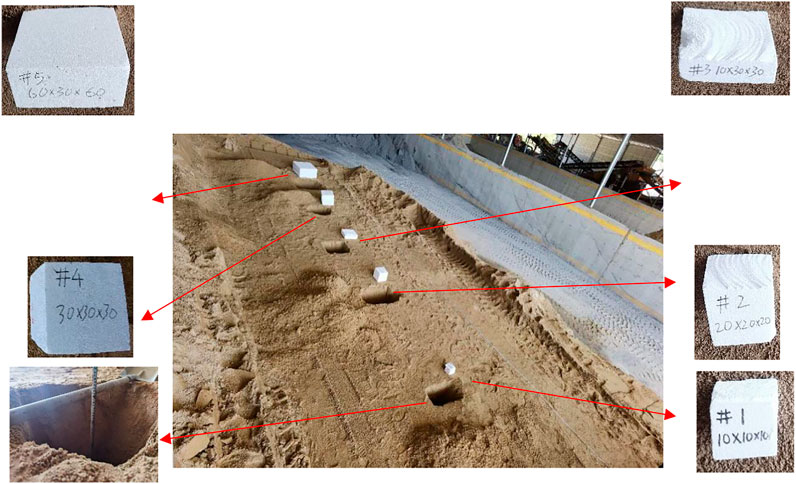
FIGURE 9. Embedding and scanning of polystyrene cubes in the test section.
In this test, river sand with a certain humidity was used as the filling material, and three parts of the 1 kg river sand in the excavated pit were taken. The water content of the river sand was determined to be 9.5% by the drying method test.
Polystyrene foam was a material that simulated the void area inside the roadbed. The empirical formula for the density and dielectric constant of polystyrene materials is shown in the following formula (Nag, 1994):
where
The density of the polystyrene material is 0.025, and the calculated dielectric constant is 1.026, which is very close to the dielectric constant 1 of the air inside the void. Therefore, polystyrene is an ideal material for simulating the void inside the road. The dielectric constant of the wet sand that simulates the propagation medium is calibrated according to its height and the double-layer travel time of the radar signal. The calibration formula is shown as follows:
where
The thickness of the straight track, the propagation time of the electromagnetic wave reflected at the air–surface interface, and the propagation time of the electromagnetic wave reflected at the bottom interface of the straight track measured at pits one to five are summarized as shown in Table 1.
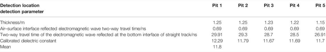
TABLE 1. Calibrated dielectric constant calculation table.
The dielectric constant of fine sand was calibrated by the layer thickness method, and the dielectric constant of fine sand was between 11.7–12.29, with an average value of 11.8, which was comparable to ordinary road construction materials (cement concrete, cement stabilized gravel, sand, etc.). Similarly, the constant was between 5 and 20.
In order to simulate the internal voids of roads of different sizes, five polystyrene cubes of different sizes were buried underground, numbered 1–5, and the side lengths were 10 cm*10 cm*10 cm (#1), 20 cm*20 cm *20 cm (#2), 30 cm*30 cm*10 cm (#3), 30 cm*30 cm*30 cm (#4), and 60 cm*60 cm*30 cm (#5). In order to avoid overlapping and mutual interference of the reflected signals between the cubes, the spacing between the polystyrene cubes was set to 200 cm, and the top surface of the polyvinyl chloride was covered with 50 cm of clay.
A three-dimensional radar antenna was used to scan the polystyrene block along the center line of the scanning area. The effective scanning width was 150 cm, and one scan could cover all the polystyrene blocks. The collected radar images were preprocessed according to the method in Section 3, the suspected void area was determined, and the three-dimensional matching was checked. The recognition result of the longitudinal section of the polystyrene cube with the largest area is shown in Figure 10.
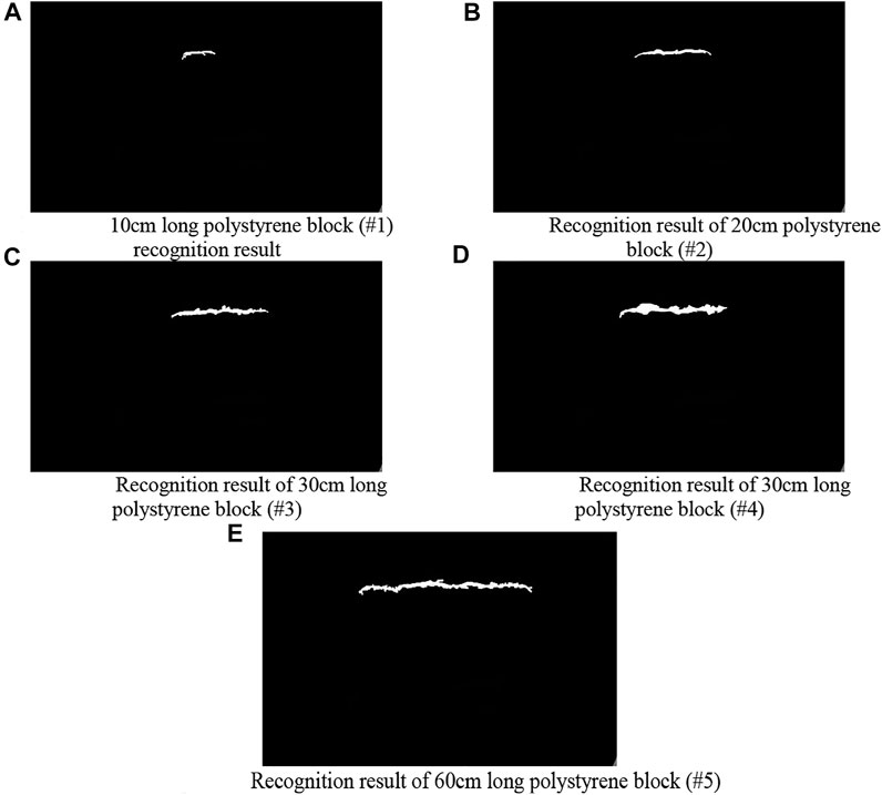
FIGURE 10. Void area recognition algorithm to identify the maximum area signal profile of the polystyrene block. (A) 10-cm-long polystyrene block (#1) recognition result. (B) Recognition result of the 20-cm polystyrene block (#2). (C) Recognition result of the 30-cm-long polystyrene block (#3). (D) Recognition result of the 30-cm-long polystyrene block. (#4) (E) Recognition result of the 60-cm-long polystyrene block (#5).
The area determined by the void area recognition algorithm was compared with the polystyrene cube site embedding position to confirm that the position was the same, and there was no false alarm area. In order to further verify the recognition accuracy of the algorithm on the volume index, the volume index recognition results of cubes with different side lengths were compared with the actual index, and the recognition error was analyzed. The result is shown in Figure 11.
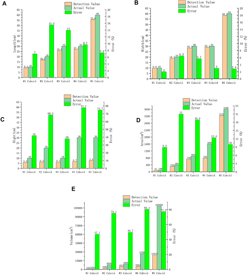
FIGURE 11. Comparison and analysis of polystyrene block volume index test results and actual values. (A) Comparison of the length of the polystyrene block with the actual value. (B) Comparison of the detection result of polystyrene block width with the actual value. (C) Comparison of the detection result of the height of the polystyrene block with the actual value. (D) Comparison of the detection result of the polystyrene block area with the actual value. (E) Comparison of the detection result of the polystyrene block volume with the actual value.
The results of error analysis between the detected volume of the polystyrene block and the actual value showed that:
1) The length detection value was generally smaller than the actual value. The detection value was on average 10.7% smaller than the actual value, and the error was between 7 and 15.5%. The weaker part of the main signal area link was cleared, causing the edge area to be cleared as a non-empty area. According to the test results, since there was no obvious correlation between the size of the error and the size of the actual value, in the subsequent algorithm application, the detection value was linearly corrected, and the correction coefficient was 1.12 (1/0.893).
2) The width detection value was also generally smaller than the actual value. The detection value was 4.0% smaller than the actual value on average, and the error was between 2 and 6.5%. The analysis reason was that the edge area signal was relatively weak, which was cleared as a non-vacant area. In the subsequent algorithm application, the detection value was corrected, and the correction coefficient was 1.04 (1/0.96).
3) The height detection value was between 5.8 and 7.6 cm, which had a large deviation from the actual value, and the error was between 42 and 77.7%. The error increases with the increase of the height of the cuboid. The reason for the analysis was that the signal reflected from the bottom of the cuboid needed to be reflected by multiple interfaces such as the vacant top interface and the air–road interface to be received by the radar receiver. After reaching the receiver, the intensity was weak, and it was interfered by signals such as multiple reflection waves. It was difficult to identify, and the original signal of #5 cuboid is shown in the following figure. Therefore, the height detection value was actually the height of the reflected signal from the top surface and could not reflect the actual height of the cube.
4) The area detection value was calculated based on the length and width. The law of deviation between the detected value and the actual value was consistent with the law of length and width, which needed to be corrected in the subsequent algorithm application, and the correction coefficient was 1.17.
5) The volume detection value was calculated based on the length, width, and height. Since the height index could not reflect the actual height of the cube, the volume detection value could not reflect the actual volume index of the cube.
In order to verify the application effect of void recognition algorithm in solid engineering, based on the test and verification of the test section, it was applied to the void collapse detection project of Huanshi Road (Nan’an Road)–Zhongshan Avenue (to Keyun Road), the main road in Guangzhou. In this project, three-dimensional ground-penetrating radar full-section coverage scanning is used to collect radar data, and void identification algorithm is used to identify void signals of radar data, and the detection results of void disease distribution in roads are obtained. According to the test results, the borehole verification work is carried out, and the identification results are compared with the actual situation inside the road obtained by borehole verification, so as to verify the application effect of void identification algorithm in solid engineering.
The detection area of the physical engineering project starts from Huanshi West Road (Xichang Interchange intersection) and ends at Zhongshan Avenue West (Keyun Road intersection), with a total length of about 15.35 km and six to fourteen lanes in both directions. The geographical location and structural layer combination are shown in Figure 12.
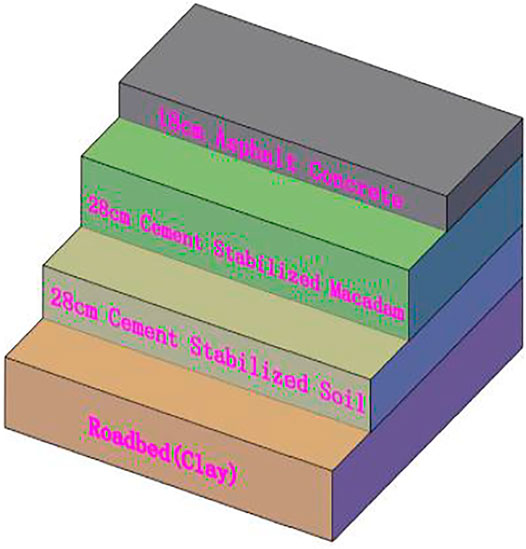
FIGURE 12. Pavement structure layer combination in the physical engineering inspection area.
The three-dimensional ground-penetrating radar system used for detection has a single detection width of 1.5 m per detection. The three-dimensional ground-penetrating radar field detection method is to divide the field road surface into several 1.5-m-wide detection lanes, which are detected in turn, and the detection sequence was recorded. After the detection is completed, the radar images of each lane are spliced according to the detection sequence to form a complete radar plan of the whole road surface. The void identification algorithm was used to process radar data, and four void diseases were identified. The field detection of physical engineering and the detection trajectory and radar image of void disease of physical engineering are shown in Figure 13.
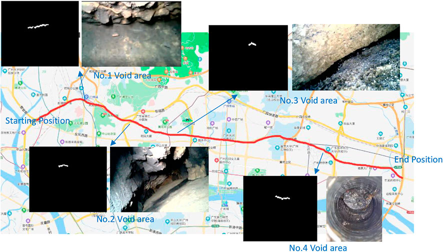
FIGURE 13. Identification and verification results of the physical engineering detection trajectory and void area.
According to the identification results, No.1 void disease is located in the soil foundation (depth is greater than 74 cm), No.2 ∼ No.3 void disease is located at the bottom of the cement concrete slab (depth is about 46 cm), and No.4 void is located at the bottom of the asphalt layer. In order to verify the accuracy of the detection results, according to the identification results and disease location, core drilling is carried out in the center of the disease point, and the field operation diagram is shown in Figure 13. At the same time, in order to confirm the internal condition of the void cavity, after drilling the hole, the internal condition map of the hole is photographed by endoscope.
After drilling verification and endoscope confirmation, all the four positions identified by the algorithm have voids, which shows that the void recognition algorithm can accurately identify the void points in radar data. The laser rangefinder is used to measure the length and width of the inner cavity of the void, and the ruler is used to measure the buried depth of the top surface of the void, which is compared with the length, width, and area of the identified void signal. The results are arranged as shown in Table 2.
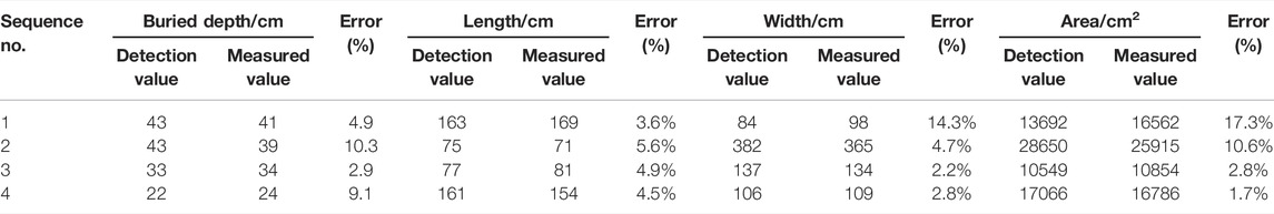
TABLE 2. Comparison between the detected volume index and measured value of the voided internal cavity.
As can be seen from the aforementioned table, the maximum error between the measured values and the measured values of the indexes such as length, width, buried depth, and area is 17.3%, and the error of most indexes is within 10%. There are still some errors in the length and width of the void area after linear correction. The reason is that the reflected signal at the link between the edge of the void area and the main area is unstable, and it is eliminated as a non-void area and retained as a void area, and the proportion of the eliminated part in the total is not a stable value, which leads to a certain deviation between the detected value and the measured value after the correction coefficient is adjusted. However, the deviation is less than 10% in general and larger in some cases, but it is still within the acceptable range of the engineering error, which shows that the volume index calculated by using void identification algorithm to process radar data has certain engineering value.
The void recognition algorithm can identify void areas by processing radar data according to a specific process and obtain radar gray images by data preprocessing; binary processing, corrosion processing, expansion processing, connected area inspection, and fine length inspection can get the suspected void area with radar image characteristics of void area; the three-dimensional matching test starts from the matching between adjacent tracks and current tracks and rechecks and confirms the identification results of void areas.
Polystyrene foam material, which is very close to the air, is used to simulate the air in the void area and the void environment of subgrade. The void recognition algorithm is used to identify the foam signal, and the recognition result is compared with the actual position and size of the buried cube. The void identification algorithm was applied to engineering projects, and four void diseases were found. The core was drilled in the center of the identified disease points, the internal conditions of the holes were photographed using an endoscope, and the length, width, and buried depth of the void internal cavity were measured. The measured results were compared with the algorithm identification results, and the results showed that:
1. Verified by the test section, the recognition result of void recognition algorithm is consistent with the buried position of polystyrene cube, and there is no error in the area. The recognition error of length is between 7 and 15%, the recognition error of width is between 2 and 6.5%, and the recognition error of area is between 8.9 and 21%;
2. Verified by the engineering project, the void identification algorithm can accurately identify the void points in radar data. The maximum error between the detected values of length, width, buried depth, and area and the measured values is 17.3%, and the error of most indexes is within 10%. The error is generally within the scope of engineering acceptance, which shows that the volume index obtained by void identification algorithm has an engineering application value.
3. In the process of project verification and test section verification, void recognition algorithm does not adjust the algorithm structure and related parameters, and the recognition results of the algorithm are consistent with the void position, which shows that the algorithm has good generalization performance. Compared with SVM, regression convolution neural network, and other recognition methods, it has the advantage of realizing void data recognition without a large amount of data training or parameter correction.
Because the reflected signal from the bottom of the void needs to be reflected by multiple interfaces such as the top interface of the void and the air–road interface to be received by the radar receiver, the intensity is weak after reaching the receiver, and it is difficult to identify because of the interference of multiple reflected waves and other signals. At present, the void recognition algorithm cannot complete the task of void bottom interface recognition. In the next stage, we can improve the quality of the radar image by optimizing radar signal processing and further summarize the image characteristics of the void bottom signal and express it by the digital image processing method to realize automatic recognition.
The raw data supporting the conclusion of this article will be made available by the authors, without undue reservation.
ZH and DW: conceptualization; GX: methodology; GX: software; GX and ZH: validation; JT: formal analysis; JT: investigation; ZH: resources; HY: data curation; HY: writing–original draft preparation; HY: writing–review and editing; DW: project administration; DW: funding acquisition. All authors have read and agreed to the published version of the manuscript.
This study is funded by the “China Postdoctoral Science Foundation” (2020M672639), the China Natural Science Foundation of Guangdong Province-PhD start (No. 2018A030310684), and the Dongguan Social Science and Technology Development (General) Project (No. 2019507140574). All help and support are greatly appreciated.
The authors declare that the research was conducted in the absence of any commercial or financial relationships that could be construed as a potential conflict of interest.
All claims expressed in this article are solely those of the authors and do not necessarily represent those of their affiliated organizations, or those of the publisher, the editors, and the reviewers. Any product that may be evaluated in this article, or claim that may be made by its manufacturer, is not guaranteed or endorsed by the publisher.
Allroggen, N., and Tronicke, J. (2020). “Ground-penetrating Radar Surveying Using Antennas with Different Dominant Frequencies,” in 18th International Conference on Ground Penetrating Radar, Golden, CO, June 14–19, 2020.
Cha, Y.-J., Choi, W., and Büyüköztürk, O. (2017). Deep Learning-Based Crack Damage Detection Using Convolutional Neural Networks. Comput. Aided Civil Infrastruct. Eng. 32 (5), 361–378. doi:10.1111/mice.12263
Domenzain, D., Bradford, J., and Mead, J. (2020). Joint Inversion of Full-Waveform GPR and ER Data Enhanced by the Envelope Transform and Cross-Gradients. Geophysics 85 (6), 1–74. doi:10.1190/gpr2020-087.1
Fenning, P. J., Jack, A. G., and Veness, J. K. (2003). “Ground Probing Radar Applications in Site Investigation,” in Proceedings of the British Institute of Non-Destructive Testing International Conference, NDT in Civil Engineering, Northampton, United Kingdom, 14-16 April, 1993 (Liverpool University).
Giertzuch, P.-L., Doetsch, J., Jalali, M., Shakas, A., and Maurer, H. (2020). Time-lapse Reflection and Transmission Borehole GPR for saline Tracer Monitoring in Fractured Rock. Geophysics 85 (3), 1–47. doi:10.1190/gpr2020-078.1
Huai, N., Zeng, Z., Li, J., Yan, Y., and Lu, Q. (2019). Model-based Layer Stripping FWI with a Stepped Inversion Sequence for GPR Data. Geophys. J. Int. 218 (2), 1032–1043. doi:10.1093/gji/ggz210
Klotzsche, A., Vereecken, H., and Kruk, J. (2019). Review of Crosshole GPR Full-Waveform Inversion of Experimental Data: Recent Developments, Challenges and Pitfalls[J]. Geophysics 84 (6), 1–66. doi:10.1190/geo2018-0597.1
Kumlu, D. (2021). Ground Penetrating Radar Data Reconstruction via Matrix Completion. Int. J. Remote Sensing 42 (12), 4607–4624. doi:10.1080/01431161.2021.1897188
Leng, Z., and Al-Qadi, I. L. (2014). An Innovative Method for Measuring Pavement Dielectric Constant Using the Extended CMP Method with Two Air-Coupled GPR Systems. NDT E Int. 66 (sep), 90–98. doi:10.1016/j.ndteint.2014.05.002
Liu, T., Zhang, X. N., Li, Z., and Chen, Z. Q. (2014). Research on the Homogeneity of Asphalt Pavement Quality Using X-ray Computed Tomography (CT) and Fractal Theory. Constr. Build. Mater. 68, 587–598. doi:10.1016/j.conbuildmat.2014.06.046
Liu, H., Shi, Z., Li, J., Liu, C., Meng, X., Du, Y., et al. (2021). Detection of Cavities in Urban Cities by 3D Ground Penetrating Radar[J]. Geophysics, 1–44. doi:10.1190/geo2020-0384.1
McGraw, D. (2020). The Measurement of the Dielectric Constant of Underground Clay Pipes[J]. Eur. J. Mater. Sci. Eng. 5 (2), 74–93. doi:10.36868/ejmse.2020.05.02.074
Nag, B. R. (1994). Empirical Formula for the Dielectric Constant of Cubic Semiconductors. Appl. Phys. Lett. 65 (15), 1938–1939. doi:10.1063/1.112823
Saarenketo, T., Nikkinen, T., and Lotvonen, S. (2014). The Use of Ground Penetrating Radar for Monitoring Water Movement in Road Structures [J]. Lett. Math. Phys. 105 (1), 1–15. doi:10.3997/2214-4609-pdb.300.88
Sarkar, R., Paul, K. B., and Higgins, T. R. (2019). Impacts of Soil Physicochemical Properties and Temporal-Seasonal Soil-Environmental Status on Ground-Penetrating Radar Response. Soil Sci. Soc. Am. J. 83 (3), 542–554. doi:10.2136/sssaj2018.10.0388
Sha, A., Tong, Z., and Gao, J. (2018). Road Surface Disease Recognition and Measurement Based on Convolutional Neural Network[J]. China J. Highw. Transport 31 (01), 1–10.
Solla, M., Lagüela, S., González-Jorge, H., and Arias, P. (2014). Approach to Identify Cracking in Asphalt Pavement Using GPR and Infrared Thermographic Methods: Preliminary Findings. NDT E Int. 62, 55–65. doi:10.1016/j.ndteint.2013.11.006
Song, I., and Larkin, A. (2016). Use of Ground Penetrating Radar at the Faa’s National Airport Pavement Test Facility (NAPTF). EGU General Assembly Conference Abstracts. doi:10.1007/978-3-319-42797-3_36
Syaifuddin, F. (2014). “Cavities Detection with Ground Penetrating Radar in limestone Dominated Rock Formation,” in PIT HAGI 39, Solo, Indonesia, October 2014.
Tang, Y.-C., Li, L.-J., Feng, W.-X., Liu, F., Zou, X.-J., and Chen, M.-Y. (2018). Binocular Vision Measurement and its Application in Full-Field Convex Deformation of concrete-filled Steel Tubular Columns. Measurement 130, 372–383. doi:10.1016/j.measurement.2018.08.026
Tang, Y., Zhu, M., Chen, Z., Wu, C., Chen, B., Li, C., et al. (2022). Seismic Performance Evaluation of Recycled Aggregate concrete-filled Steel Tubular Columns with Field Strain Detected via a Novel Mark-free Vision Method. Structures 37, 426–441. doi:10.1016/j.istruc.2021.12.055
Tang, J. (2020). Research on Asphalt Pavement Construction Quality Evaluation and Control Based on 3D Ground Penetrating Radar. South China University of Technology.
Tong, Z., Sha, A-M., and Gao, J. (2017). Innovation for Recognition of Pavement Distresses by Using Convolutional Neural Network. Beijing, China: World Transport Convention.
Tosti, F., and Ferrante, C. (2020). Using Ground Penetrating Radar Methods to Investigate Reinforced Concrete Structures. Surv. Geophys. 41 (3), 485–530. doi:10.1007/s10712-019-09565-5
Wang, S., Zhao, S., and Al-Qadi, I. L. (2020). Real-Time Density and Thickness Estimation of Thin Asphalt Pavement Overlay during Compaction Using Ground Penetrating Radar Data[J]. Surv. Geophys. 41 (6), 431. doi:10.1007/s10712-019-09556-6
Wang, S., Al-Qadi, I. L., and Cao, Q. (2020). Factors Impacting Monitoring Asphalt Pavement Density by Ground Penetrating Radar. NDT E Int. 115, 102296. doi:10.1016/j.ndteint.2020.102296
Wu, F., Duan, J., Chen, S., Ye, Y., Ai, P., and Yang, Z. (2021). Multi-Target Recognition of Bananas and Automatic Positioning for the Inflorescence Axis Cutting Point. Front. Plant Sci. 12, 705021. doi:10.3389/fpls.2021.705021
Yan, P., Capus, C., Brown, K., and Petillot, Y. (2011). “Biosonar: a Bio-Mimetic Approach to Sonar Systems Concepts and Applications,” in On Biomimetics (InTech).
Zhou, H., Jiang, Y., Xu, L., and Liang, G. (2013). Automatic Detection Algorithm of Highway Subgrade Diseases Based on SVM[J]. China J. Highw. Transport 26 (02), 42–47.
Keywords: 3D radar, image, void, identification, nondestructive test
Citation: Huang Z, Xu G, Tang J, Yu H and Wang D (2022) Research on Void Signal Recognition Algorithm of 3D Ground-Penetrating Radar Based on the Digital Image. Front. Mater. 9:850694. doi: 10.3389/fmats.2022.850694
Received: 08 January 2022; Accepted: 21 February 2022;
Published: 30 March 2022.
Edited by:
Hui Yao, Beijing University of Technology, ChinaReviewed by:
Hasimah Ali, Universiti Malaysia Perlis, MalaysiaCopyright © 2022 Huang, Xu, Tang, Yu and Wang. This is an open-access article distributed under the terms of the Creative Commons Attribution License (CC BY). The use, distribution or reproduction in other forums is permitted, provided the original author(s) and the copyright owner(s) are credited and that the original publication in this journal is cited, in accordance with accepted academic practice. No use, distribution or reproduction is permitted which does not comply with these terms.
*Correspondence: Jiaming Tang, 136225548@qq.com
Disclaimer: All claims expressed in this article are solely those of the authors and do not necessarily represent those of their affiliated organizations, or those of the publisher, the editors and the reviewers. Any product that may be evaluated in this article or claim that may be made by its manufacturer is not guaranteed or endorsed by the publisher.
Research integrity at Frontiers
Learn more about the work of our research integrity team to safeguard the quality of each article we publish.