Seasonal and interannual variabilities of the thermal front east of Gulf of Thailand

Based on satellite-observed and reanalysis data, this study investigates a thermal front east of the Gulf of Thailand (TFEGT) during the winter from 1982 to 2021. TFEGT exhibits distinct seasonal and interannual variation, emerging in December, peaking in February, gradually diminishing in March, and completely dissipating in April. Notably, the occurrence probability, area, and intensity of the thermal front are significantly higher in January and February compared with December and March. Through the application of a mixed temperature equation, we identify that geostrophic advection, driven by wind-induced western boundary current in the South China Sea (SCS), plays a crucial role in the formation of the TFEGT. In winter, the prevailing northeast monsoon propels the western boundary current through wind stress curl, causing the southward transport of cold water from north to south. This cold water encountered warm water within the Gulf of Thailand (GoT), leading to the formation of TFEGT. Furthermore, the interannual variation of TFEGT is closely associated with the El Niño-Southern Oscillation (ENSO). In El Niño (La Niña) years, the northeast monsoon weakens (enhances), resulting in a weaker (stronger) western boundary current, ultimately influencing the weakening (enhancement) of TFEGT.

1 Introduction

The ocean thermal front is a relatively narrow transitional zone between two or more adjacent water masses with significant temperature differences (Ullman and Cornillon, 1999). As an essential physical feature in the ocean, the thermal front plays a pivotal role in marine ecosystems, heat transport, and fishery production (Belkin et al., 2009; Woodson and Litvin, 2015). The mechanism governing its occurrence and spatiotemporal variations often unveil insights into ocean circulation development and atmospheric signals. Furthermore, it sheds light on interaction between the ocean and the atmosphere, involving frequent exchanges of momentum, heat, and water vapor (Chelton et al., 2007). In the sea–air interaction system, the ocean primarily influences weather by transporting heat to the atmosphere, whereas the atmosphere predominantly alters the direction of ocean currents and the heat content of seawater through wind stress. The thermal front is significantly influenced by weather and climate changes, and it can reciprocally impact the atmospheric system, interfering with the operation of weather systems at sea and on land. Propelled by the dynamic mechanism, the regions where the front occurs accumulate abundant plankton and nutrients, attracting the aggregation of diverse fish species.

The SCS is the largest semi-enclosed marginal sea in the northwest Pacific Ocean, enveloped by the Asian mainland and numerous islands and interconnected with the Pacific Ocean through the Luzon Strait (Hu et al., 2000). Situated within the Asian monsoon region, the transition of monsoons serves as the decisive factor in determining the upper ocean circulation of the SCS (Xue et al., 2004; Liu et al., 2008). During the summer, the prevailing southwest monsoon induces cyclonic circulation in the north and anticyclone circulation in the south. Conversely, in winter, the northeast monsoon dominates the air over the SCS, with the strongest wind stress observed during this season (Qu et al., 2007). The intensified wind results in severe wave agitation, causing uplift of bottom seawater and deepening of the mixed layer (Gao and Wang, 2008). Additionally, it triggers cyclonic circulation throughout the entire SCS basin. These distinctive sea–land structures and climatic characteristics contribute to the richness of thermal fronts in the SCS. The thermal fronts predominantly manifest along the northern coast, with the northern shelf serving as their primary aggregation zone. Other notable locations include the eastern coast of Vietnam, surrounding areas of Hainan Island, Taiwan Strait, and Luzon Strait. Along the Guangdong coast, the downward flow driven by the northeast monsoon in winter converges with coastal seawaters, leading to the formation of abundant thermal fronts. In the eastern part of Vietnam and Hainan Island, wind stress emerges as a key determinant for thermal front occurrence, whereas the upwelling caused by the southwest monsoon in summer leads to front formation. Various dynamic processes, including wind stress curl, mesoscale eddies, and Kuroshio intrusion, contribute to the emergence of thermal fronts in the northwest of Luzon Island (Wang et al., 2020). The thermal fronts in the Taiwan Strait and adjacent regions exhibit strength during winter, with tidal mixing, hydrological characteristics, and monsoon-induced seawater transport identified as crucial factors for their appearance (Li et al., 2006; Pi and Hu, 2010). In summary, a robust feedback mechanism exists between the generation and disappearance of thermal fronts in the SCS and the Asian monsoon (Wang et al., 2012), with significant seasonal disparities and complex frontal structures (Zhu et al., 2014). Furthermore, this interaction is also influenced by wind stress and ENSO, resulting in fluctuating interannual variations (Yu et al., 2019; Wang et al., 2020). Belkin and Cornillon (2003) determined thermal fronts along the Pacific coast and marginal sea areas, noting the occurrence of a narrow thermal front in the eastern part of the GoT southwest of the SCS during the winter.

The GoT is situated to the southwest of the SCS (Figure 1), between the Indo-China Peninsula and the Malay Peninsula. Numerous inland streams and rivers converge here and discharge water directly into the gulf (Snidvongs, 1998). Its southeast is connected to the main region of the SCS; therefore, the circulation in the GoT is mainly controlled by the Asian monsoon and the SCS circulation. During the southwest monsoon, a clockwise circulation prevails near the gulf top. The central part of the gulf experiences a robust anticyclonic circulation, with the current flowing northward from the SCS along the Malay Peninsula into the GoT before exiting to the northeast (Aschariyaphotha et al., 2008). The mouth of the gulf exhibits a semi-counterclockwise circulation. In contrast, during the northeast monsoon, the SCS current enters the GoT along the southern Vietnam coast from the northeast to the southwest. The circulation inside the gulf remains predominantly clockwise, whereas the eastern part of the gulf demonstrates counterclockwise circulation (Penyapol, 1957; Wyrtki, 1961; Yanagi and Takao, 1998; Buranapratheprat et al., 2002). In winter, the northeast monsoon in the northern hemisphere drives the low-temperature and high-salinity seawater from the northern SCS to the southwest (Aschariyaphotha et al., 2008), leading to accumulation of seawater in the GoT (Chu et al., 1999). Simultaneously, warm water with low salinity converges around the upstream of the GoT, inducing a gradual cooling of seawater in the gulf from the interior to the exterior (Tang et al., 2006; Li et al., 2014). Based on the previous experience and research, it is evident that the formation and variation of the TFEGT in winter are closely linked to the monsoon and the circulation of the SCS (Belkin and Cornillon, 2003). However, the spatiotemporal variation characteristics and dynamic mechanisms of its formation are still unclear, prompting a detailed study in this paper. Winter in this paper is defined as the period from December to March of the following year. The rest of this paper is organized as follows. Section 2 provides a brief introduction to the research data and methods. Section 3 presents the seasonal and interannual variation characteristics of the front, along with discussions on the dynamic mechanisms of TFEGT’s formation and variability. Section 4 summarizes all the results obtained from this study.

Figure 1

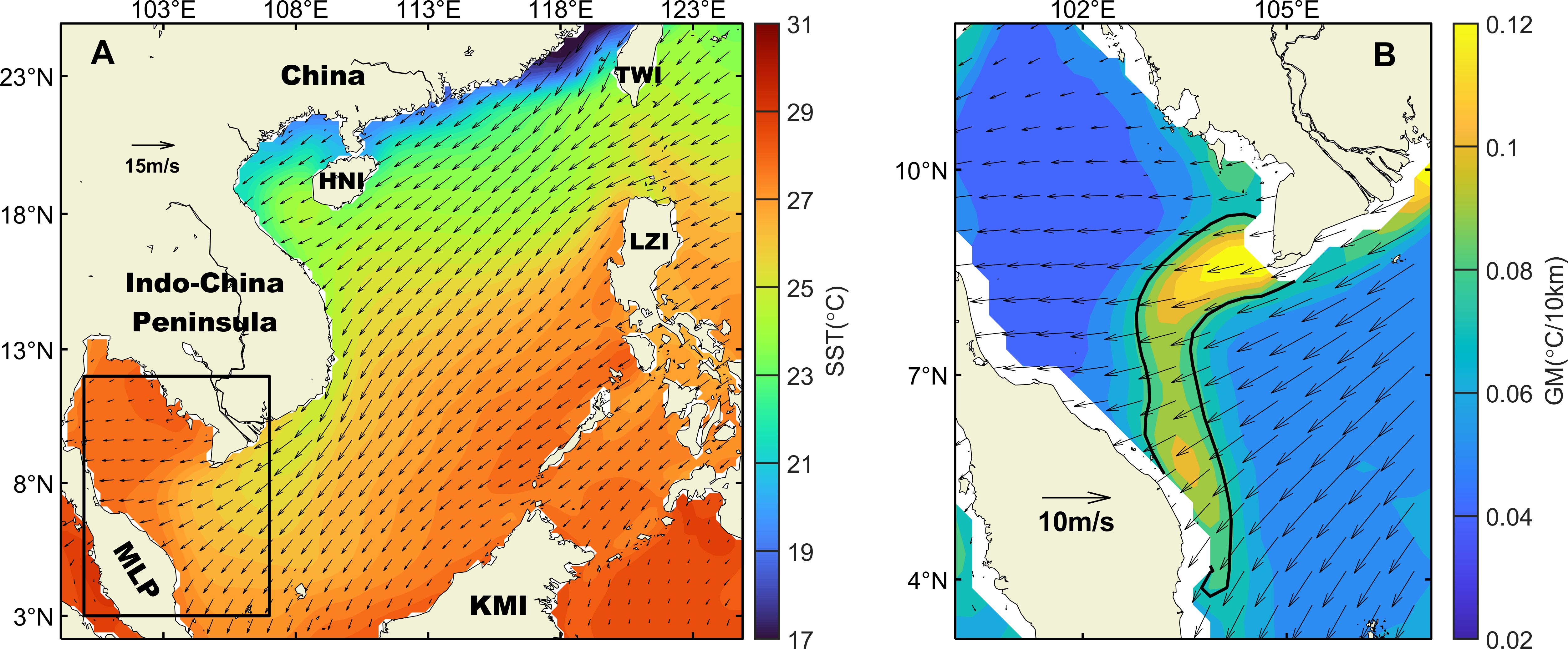
Figure 1 (A) Topographic distribution of the SCS and climatological distribution of sea surface temperature (SST) (°C, in color) and wind vectors (m/s, in vector) in winter from 1982 to 2021. The black box is the study area of TFEGT. TWI, Taiwan Island; HNI, Hainan Island; MLP, Malay Peninsula; KMI, Kalimantan Island; LZI, Luzon Island. The black box is the study area of the TFEGT. (B) Winter climatological mean distribution of gradient magnitude (GM) (°C/10 km, shading) and wind vectors (m/s, in vector) in GoT. The black solid lines represent the contour line with GM of 0.08°C/10 km.

2 Data and methods

2.1 Data

The daily sea surface temperature data were from the Optimal Interpolation Sea Surface Temperature (OISST) dataset provided by the National Oceanic and Atmospheric Administration (NOAA) (Reynolds et al., 2007). OISST is a long-time climate data record, which incorporates the observation results of SST from different platforms including satellites, ships, buoys, and Argo floats into a regular global grid, and then fills the gaps on the grid with the interpolation method to create a complete global SST map. Satellite and ship observations are referenced to buoys to compensate for platform differences and sensor biases. The OISST dataset provides global SST from 01/01/1982 to present, with a spatial resolution of 0.25° × 0.25° and a temporal sampling frequency of 1 day (Huang et al., 2021).

Surface ocean net heating flux data and sea water potential temperature data came from the Simple Ocean Data Assimilation (SODA) dataset generated by the Global Simple Ocean Data Assimilation Analysis System. SODA was developed by the University of Maryland in the early 1990s to provide a set of ocean reanalysis data that matches atmospheric reanalysis data for climate research (Carton and Giese, 2008). It contains variables temperature, salinity, current vector, sea surface wind stress, sea surface heat content, sea level height, etc. With the continuous development and upgrading of assimilation systems, there are multiple versions of the dataset, and version 3.15.2 was downloaded in this paper. This version uses the ERA5 meteorological forcing set and includes assimilation reanalysis with CORE2, DFS5.2, JRA-55DO, and flux bias correction applying the COARE4 bulk formula. It provides every 5-day global ocean data from 03/01/1980 to the present with a horizontal resolution of approximately 1/4° × 1/4° and a temporal resolution of 5 days, and 50 standard depths from the surface to nearly 5,500 m with a vertical resolution varying from 5 m at the surface to 200 m below 2,000 m (Carton and Giese, 2005; Jackett et al., 2006; Carton et al., 2018).

The monthly climatological mean mixed layer depth data were from World Ocean Atlas 2018 (WOA2018). It is generated by situ profile data from 1981 to 2017 and calculated for each profile by estimating the depth for which the potential density at 10 m (reference depth) increases by 0.125 kg/m³ (Locarnini et al., 2018). The dataset has a global product with a horizontal resolution of 0.25° × 0.25°.

Surface geostrophic velocity data were obtained from Copernicus Marine Environment Monitoring Service (CMEMS). The dataset is produced from the processing system, whose data are measured by multi-satellite altimetry observations over global ocean including Topex/Poseidon, Jason-1, OSTM/Jason-2, Jason-3, and ERS-1. It provides data from 1993 to the present with a spatial resolution of 0.25° × 0.25° and a temporal sampling frequency of 1 day. The CMEMS generates a near real-time component and a delayed-time component. This paper chooses the delayed-time component, which contains all altimeter data with homogeneous, inter-calibrated, and highly accurate long time series (Pujol, 2022).

Geostrophic velocity data came from the Cross-Calibrated Multi-Platform (CCMP) version 2.0 ocean vector wind dataset provided by Remote Sensing Systems (RSS). It combines inter-calibrated satellite remote sensing observation data from numerous radiometers and scatterometers, in situ observation data from moored buoys, and model wind data by using multiple analysis methods. The dataset provides near-global gridded dataset of surface wind vectors spanning August 1987–present, with a spatial resolution of 0.25° × 0.25° and a temporal sampling frequency of 6 h (Atlas et al., 2011; Mears et al., 2019). All wind observations (satellite and buoy) and model analysis fields are referenced to a height of 10 m (Wentz et al., 2015).

2.2 Methods

2.2.1 Definition of thermal fronts

The identification of thermal fronts in marine environments conventionally involves computing the gradient magnitude (GM) of the horizontal temperature gradient at the sea surface. When the GM of an area surpasses or equals a specific threshold, it is inferred that a thermal front is present within the designated region (Chang et al., 2010). The formulation employed for GM calculation in this study is as follows:

$\begin{array}{ll}\begin{array}{c}GM=\sqrt{{\left(-\frac{\partial T}{\partial x}\right)}^2+{\left(-\frac{\partial T}{\partial y}\right)}^2},\end{array}& (1)\end{array}$

where $GM$ is the value of gradient magnitude, T is SST, $x$ and $y$ axes are directed toward the east and north, respectively. By calculating the winter climatology GM value of the GoT and adjacent waters, we found that there is a clear boundary between the area with GM ≥0.08°C/10 km and the other area. Therefore, 0.08°C/10 km is selected as the threshold of the TFEGT according to the previous experience and the specific situation of the thermal front on account of maximizing the manifestation of its distinctive features. The thermal front in this paper was calculated using OISST with a spatial resolution of 0.25° × 0.25° as described in Section 2.1, and we also calculated the thermal front with MODIS SST with a spatial resolution of 4 km × 4 km. The spatial distribution of the thermal front calculated by both is consistent.

The front area is defined as the total area where GM calculated by Equation 1 surpasses or equals the threshold within the framed region. The front intensity is defined as the arithmetic mean of all GM values in the framed region. The probability of front occurrence is defined as the ratio of the days when a front is observed to the total observation days at a certain grid point in the framed region, and then multiplied by 100%. These statistical indicators find widespread application in diverse studies of ocean fronts, providing a lucid and intuitive portrayal of front variations across different dimensions (Chang et al., 2010; Sun et al., 2015).

2.2.2 Mixed-layer temperature equation

The distribution and evolution of thermal fronts are intricately related to SST. Therefore, an investigation into the mechanisms governing front occurrence can be initiated by scrutinizing the factors that influence SST changes. In order to quantitatively evaluate the impact of various marine dynamic factors on SST, the following mixed-layer temperature equation is applied in this paper (Qu, 2000):

$\begin{array}{ll}\begin{array}{c}\frac{\partial T}{\partial t}=\frac{Q}{\rho C_p{h}_m}-u_e·\nabla T_m-u_g·\nabla T_m-\frac{W_{ent}(T-T_d)}{h_m},\end{array}& (2)\end{array}$

where $T$ is the SST, which is very similar to the temperature of the mixed layer, $t$ is the time, $Q$ is the surface net heat flux, $\rho$ is the reference density of seawater, $\rho C_p$ is the specific heat capacity per unit volume, $h_m$ is the depth of mixed layer, $u_e$ is Ekman velocity, $u_g$ is the geostrophic velocity, $W_{ent}$ is the vertical entrainment velocity, and $T_d$ is the water temperature at 5 m below the mixed layer. Equation 2 is divided into five terms from left to right, which are the temperature tendency term, net surface heat flux term, Ekman heat advection term, geostrophic heat advection term, and vertical heat entrainment term.

3 Results

3.1 Seasonal variation of the TFEGT

Figure 2 shows the presence of a thermal front in the southeast of the GoT from December to March, defined as TFEGT. The front begins to form in December, reaches peak prominence in February of the following year, decays in March gradually, and completely dissipates in other months. There are two GM peaks positioned at both extremities of the front, approaching the shores and decreasing toward the surrounding areas gradually. For quantitatively describing the variation characteristics and development trends of the front, we demarcated a specific front area using the coasts at both ends and black full lines based on the winter climate state GM of 0.08°C/10 km (Figure 1B). The enclosed region almost covers all the areas where the front occurs, so the characteristics of the TFEGT variation this article will statistically analyze next specifically refer to the thermal front within this region.

Figure 2

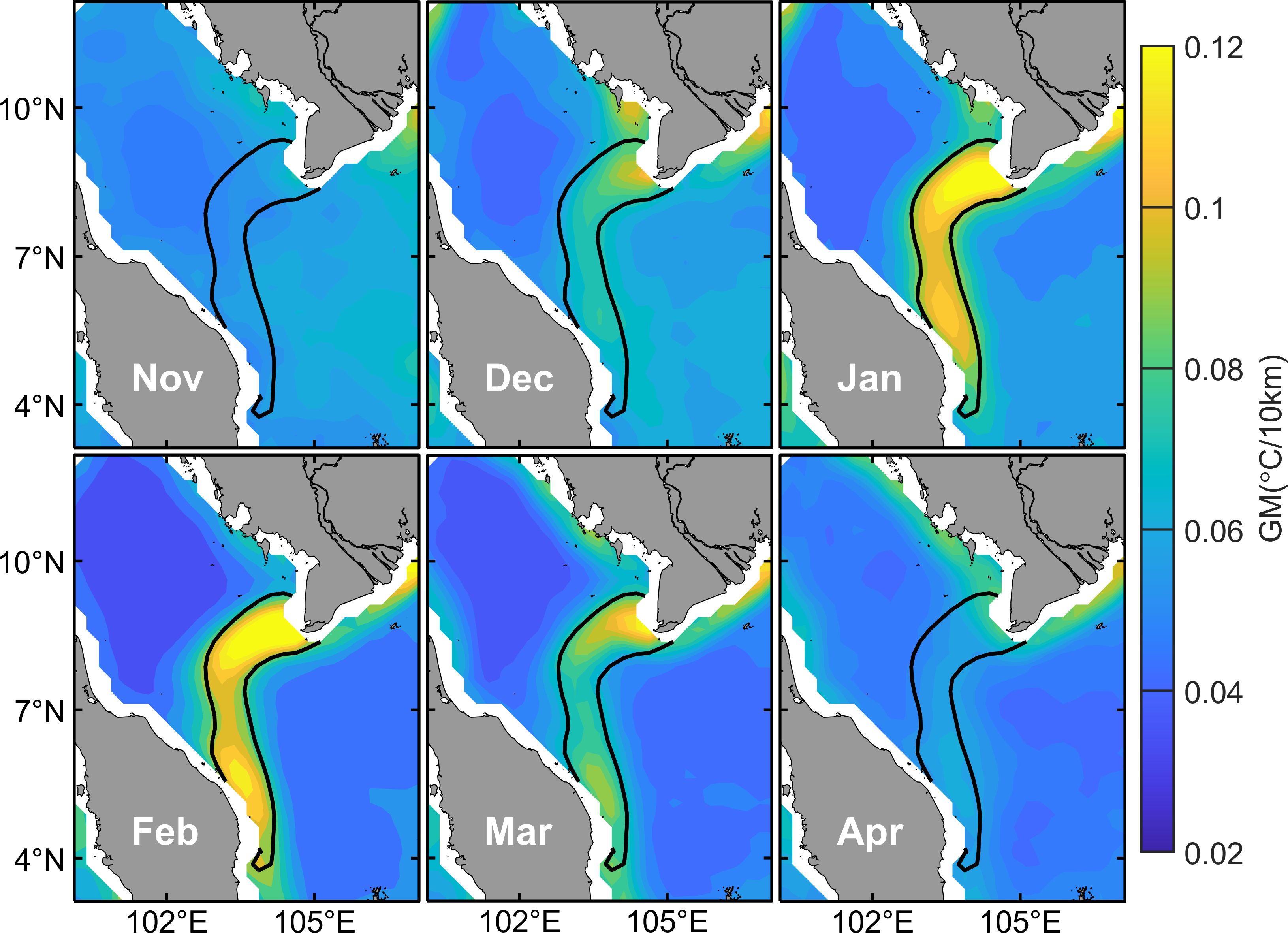
Figure 2 Monthly variation from November to April of GM (°C/10 km, shading). The definition of the black solid lines is consistent with that in Figure 1B.

To clarify the seasonal variabilities of the TFEGT, this paper cites three indicators: probability, area, and intensity of the front. Figure 3 displays the probability variation of the front from December to March. It can be seen that the probabilities of TFEGT are consistently above 30%. On the temporal scale, the front arises most frequently in January and February. The probability of occurrence mostly exceeds 60%, and the high value can reach around 80%. That is notably greater than the probabilities in other 2 months. The probability of occurrence in December and March is relatively lower, mainly fluctuating between 40% and 50%. On the spatial scale, the likelihood of the front occurring near the coast at both ends is highest and gradually diminishes toward the middle.

Figure 3

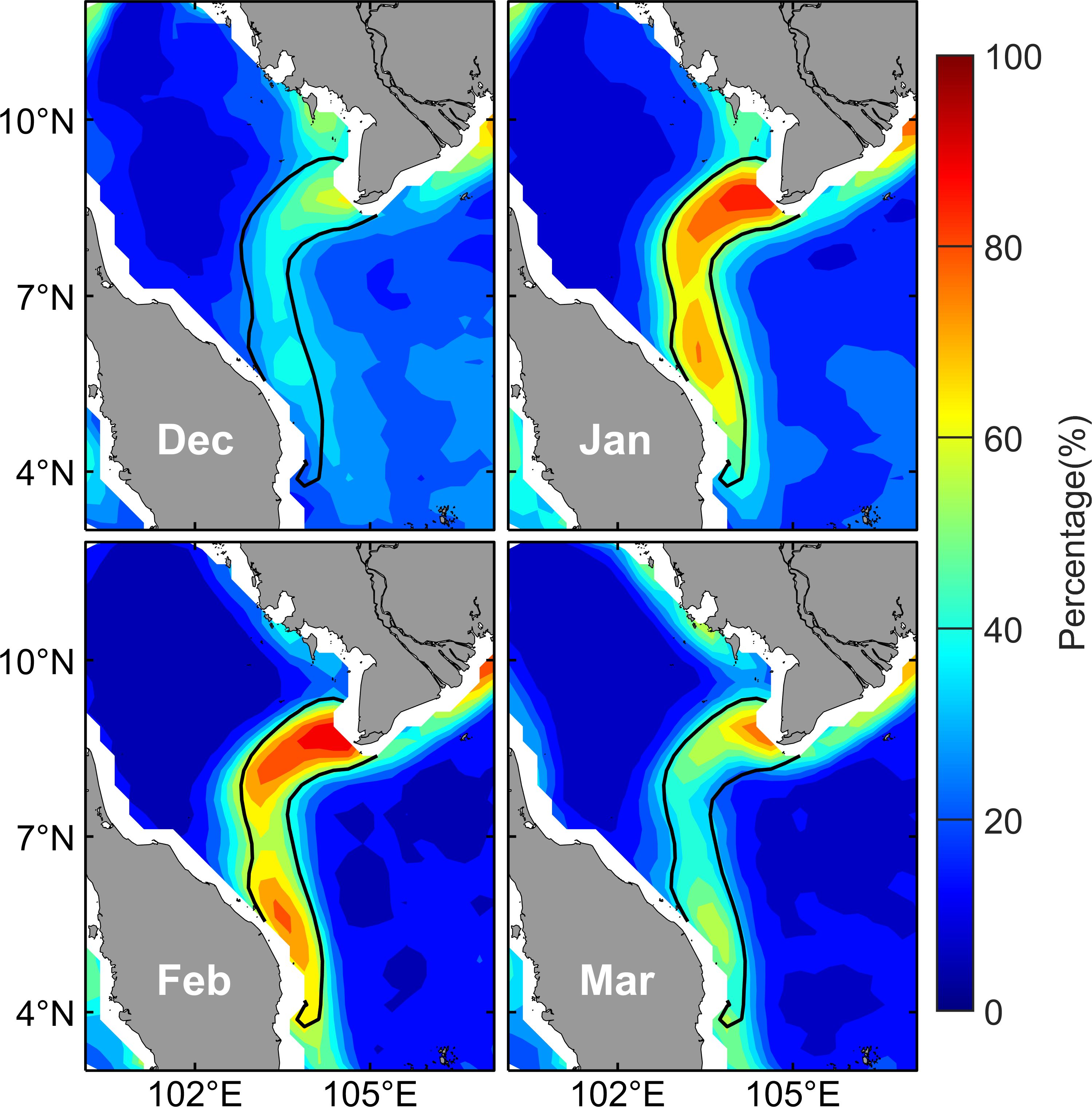
Figure 3 Mean front occurrence probability of the TFEGT from December to March during 1982–2021 (%, color shading). The definition of the black solid lines is consistent with that in Figure 1B.

Figure 4 shows the monthly average area and intensity of TFEGT from December to March, with the areas ranging from 2.2 × 10⁴ km to 4.2 × 10⁴ km² and the intensities ranging from 0.07°C to 0.12°C/10 km. A notably high positive correlation is evident between the variation of the area and intensity. The larger the front area in a given month, the stronger the intensity. Consistent with the pattern presented by occurrence probability, both the area and intensity of the TFEGT exhibit significant increases in January and February compared with December and March. They are rapidly increasing from December to January, relatively stable from January to February, and subsequently decreasing from February to March.

Figure 4

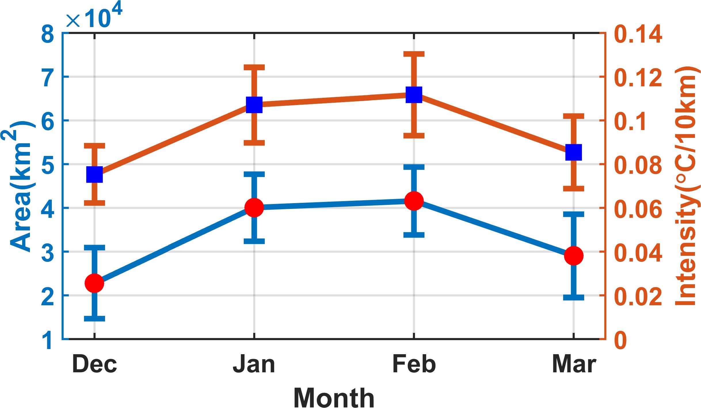
Figure 4 Monthly variation of area (km², in blue) and intensity (°C/10 km, in orange) of the thermal front with their standard deviations from December to March.

3.2 Interannual variation of the TFEGT

The interannual variation of the TFEGT is very pronounced (Figure 5). Figure 6A presents the area of TFEGT in winter from 1982 to 2021. From the trend perspective, before 2006, the interannual fluctuation of front area in winter is relatively flat except for 1996–1998 and then becomes very intense after 2010. The fronts in 1995, 2007, 2017 and 2019 (1997, 2009, 2012, 2015, and 2018) are selected, where the front area is larger (smaller) than the sum (difference) of the one-time standard deviation and the average value of the area in winter from 1982 to 2021 to composite into a strong (weak) front area type (Figures 6B, C). The area of the strong front area type can reach 4.08 × 10⁴ km², whereas the area of the weak front area type is 2.31 × 10⁴ km², less than two-thirds of the strong front area type. Figure 7A presents the intensity of TFEGT in winter from 1982 to 2021; its interannual variation is very analogous to the area. The fronts in 1983, 1984, 1995, 2007, 2010, 2011, and 2019 (1997, 2009, 2015, and 2018) are selected, where front intensity is greater (less) than the sum (difference) of the one-time standard deviation and the average value of intensity in winter from 1982 to 2021 to composite into a strong (weak) front intensity type (Figures 7B, C). The intensity of the strong front intensity type is 0.11°C/10 km, and the intensity of the weak front intensity type is merely 0.07°C/10 km, approximately two-thirds of the strong front intensity type. The correlation coefficient between front area and intensity is 0.97, which has passed the 95% confidence level. This signifies a highly consistent trend in the variations of front area and intensity, with greater intensity corresponding to a larger front area.

Figure 5

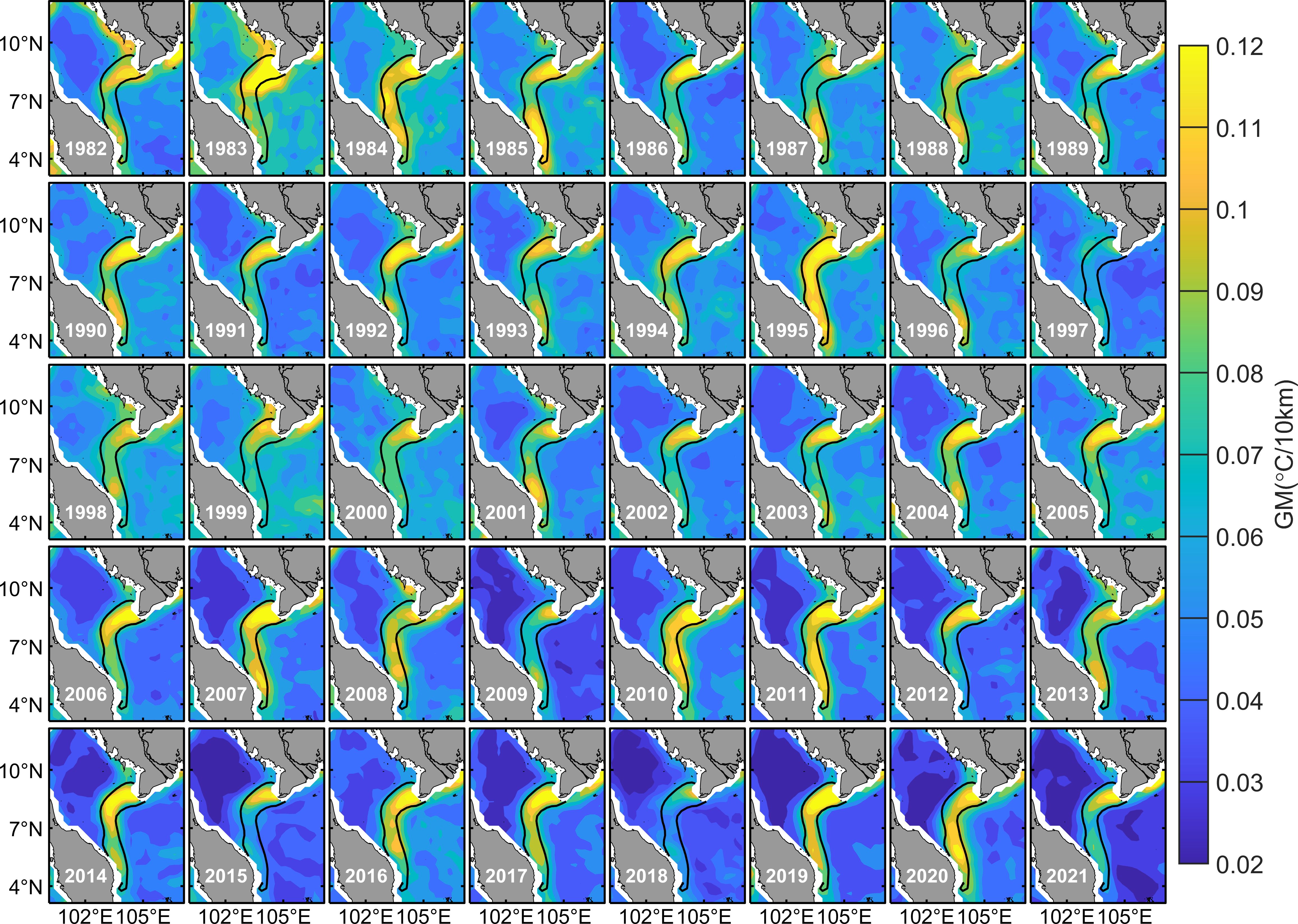
Figure 5 Mean annual GM of the TFEGT from 1982 to 2021 (°C/10 km, color shading). The definition of the black solid lines is consistent with that in Figure 1B.

Figure 6

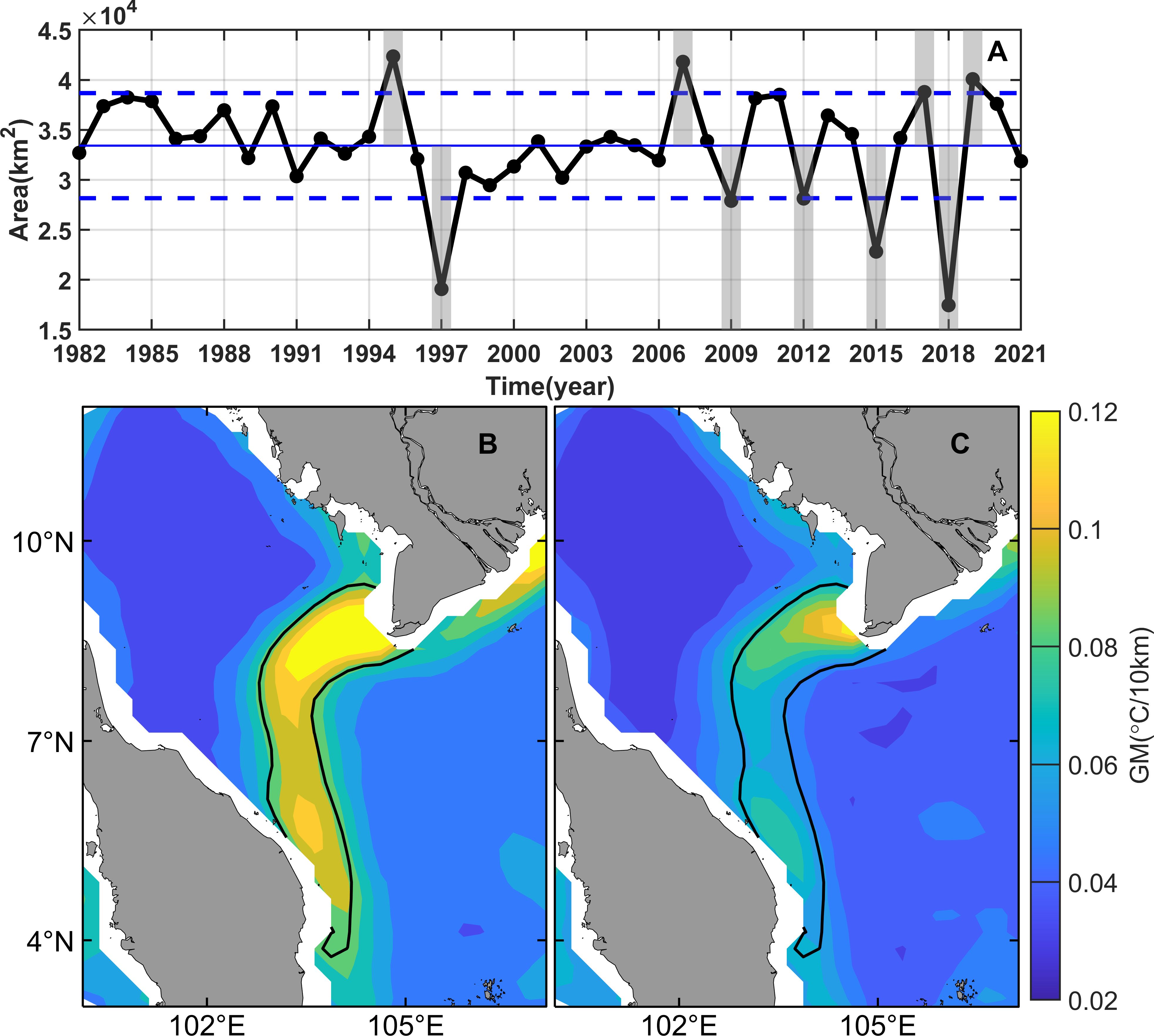
Figure 6 (A) The time series of annual thermal front area in winter from 1982 to 2021. The upper (lower) dashed blue line represents the sum (difference) of the one-time standard deviation and the average value of the time series, and the years when the time series is bigger (smaller) than the upper (lower) dashed blue line are defined as greater (weaker) area years. (B) Spatial distribution of the thermal front in greater area years. (C) is the same as (B), but for weaker area years. The definition of the black solid lines is consistent with that in Figure 1B.

Figure 7

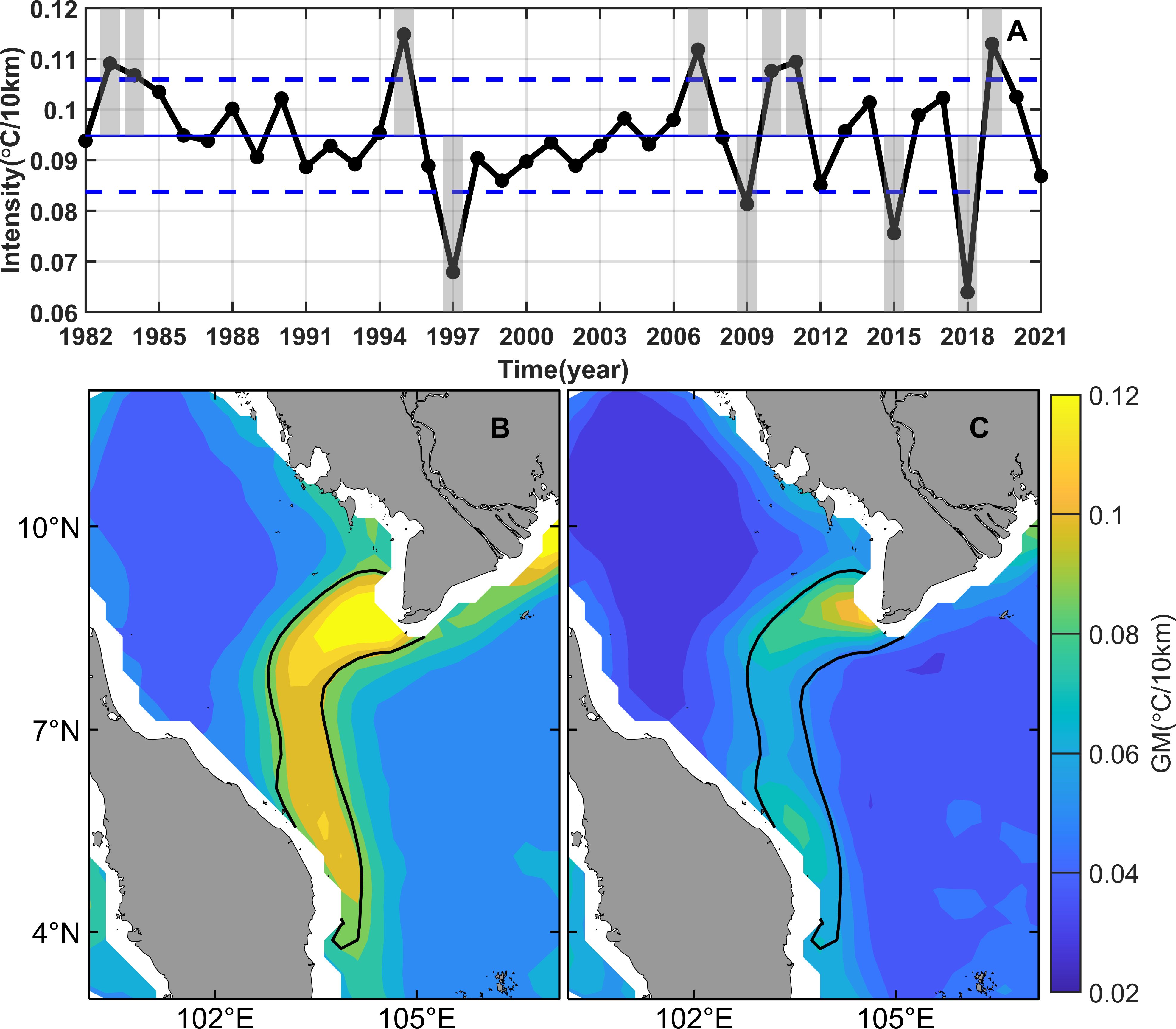
Figure 7 (A) The time series of annual thermal front intensity in winter from 1982 to 2021. The upper (lower) dashed blue line represents the sum (difference) of the one-time standard deviation and the average value of the time series, and the years when the time series is bigger (smaller) than the upper (lower) dashed blue line are defined as greater (weaker) intensity years. (B) Spatial distribution of the thermal front in greater intensity years. (C) is the same as (B), but for weaker intensity years. The definition of the black solid lines is consistent with that in Figure 1B.

The climate in the entire SCS has always been strongly influenced by ENSO (Fang et al., 2006; Wang et al., 2006). As shown in Figure 8A, there exists a notable correspondence between the intensity of TFEGT and the Niño3 index. Figure 9 is the correlation coefficient curve between the Niño3 index and the intensity of the TFEGT for leading and lagging 1–12 months. The maximum negative correlation coefficient is −0.58 when the Niño3 index leads the intensity by 2 months, implying that the thermal front has a delayed response to ENSO. Figures 8B, C represent an El Niño (a La Niña) front type composited by the TFEGTs in strong El Niño (La Niña) years with Niño 3 index greater (less) than 1 (−1), including 1982, 1987, 1997, and 2015 (1988, 1998, 2007, 2010, and 2020), The intensity of TFEGT in the El Niño type is markedly less than in the La Niña type, that means El Niño (La Niña) acts as an inhibiting (promoting) factor in the formation of the thermal front. The specific dynamic mechanism between them will be further studied in Section 3.3.

Figure 8

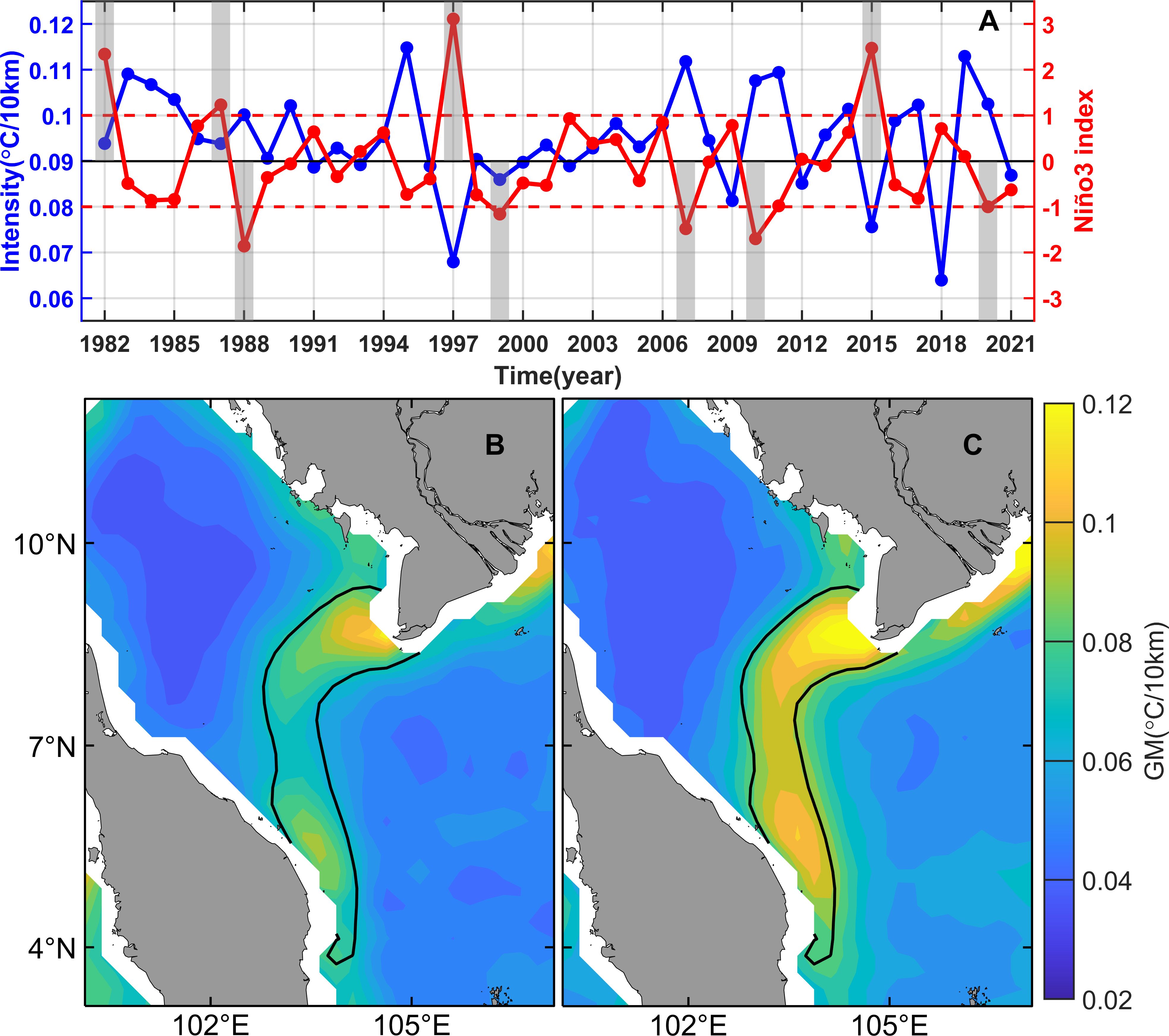
Figure 8 (A) The time series of annual thermal front intensity (in blue) and Niño3 index (in red) from 1982 to 2021. The upper (lower) dashed red line represents is where the Niño 3 index is 1(−1). The upward (downward) gray bar shadows represent years with the Niño 3 index greater than 1 (less than −1). (B) A composite El Niño front type of TFEGT (°C/(10 km), color shading). (C) is the same as (B), but for the La Niña front type. The definition of the black solid lines is consistent with that in Figure 1B.

Figure 9

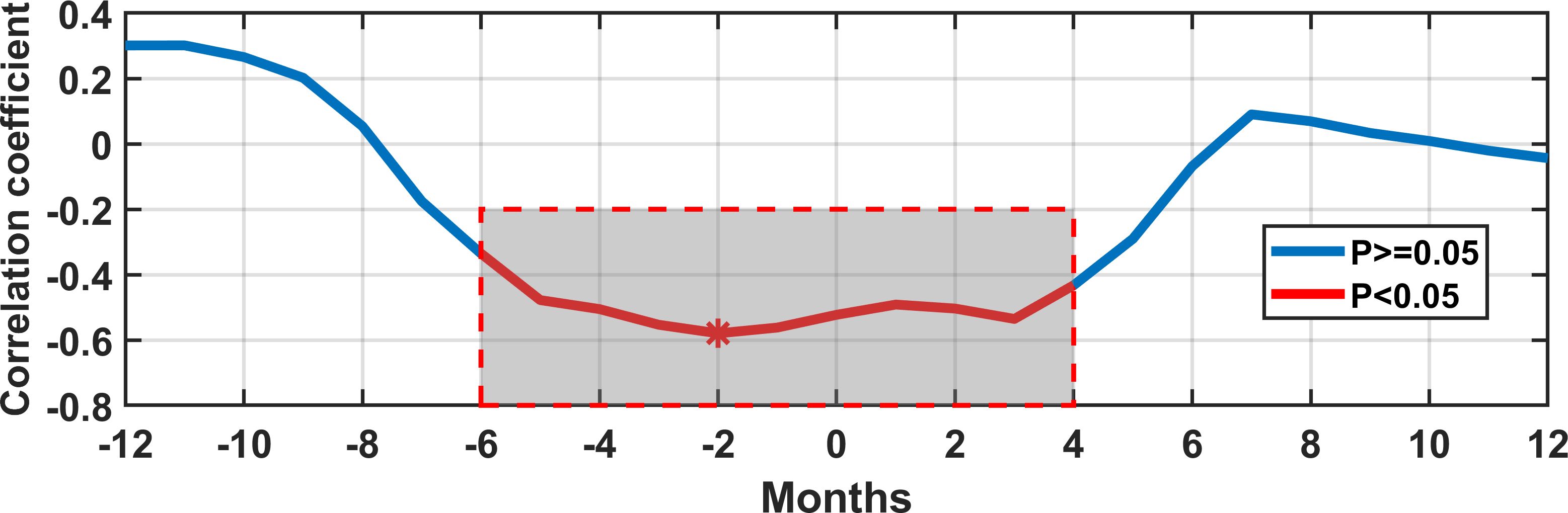
Figure 9 The correlation coefficient of the Niño3 index leading (months<0) and lagging (months >0) the front intensity for 1–12 months. The red line in the shadow represents the part that has passed the 95% confidence level. The ''*" means the position with the highest correlation coefficient in the shadow area.

3.3 Formation mechanism of the TFEGT

In order to explore the drivers of the TFEGT, this paper selects a square region on each side of the front zone based on terrain and frontal morphology. The red box A (B) in Figure 10 represents the sea area on the west (east) of the TFEGT, approximately located in the middle of the current water area. Figure 11 shows the climatological SST difference between the east and west sides of the thermal front from December to March. Comparing the SST difference with the intensity of TFEGT, the two indexes emerge a meaningful corresponding relationship: In December and March (January and February), when the front intensity is relatively small (large), the SST difference is also relatively small (large). Figure 12 displays the annual variation of the average SST difference and the front intensity in winter from 1982 to 2021. Both variables exhibit a consistent trend with a correlation coefficient of 0.83 and have passed the 95% confidence level, meaning that the SST difference between the two sides of the TFEGT can effectively characterize the intensity of TFEGT. Therefore, the investigation into the formation mechanism of TFEGT can commence by explaining the dynamic mechanism governing the spatial distribution of SST around the GoT.

Figure 10

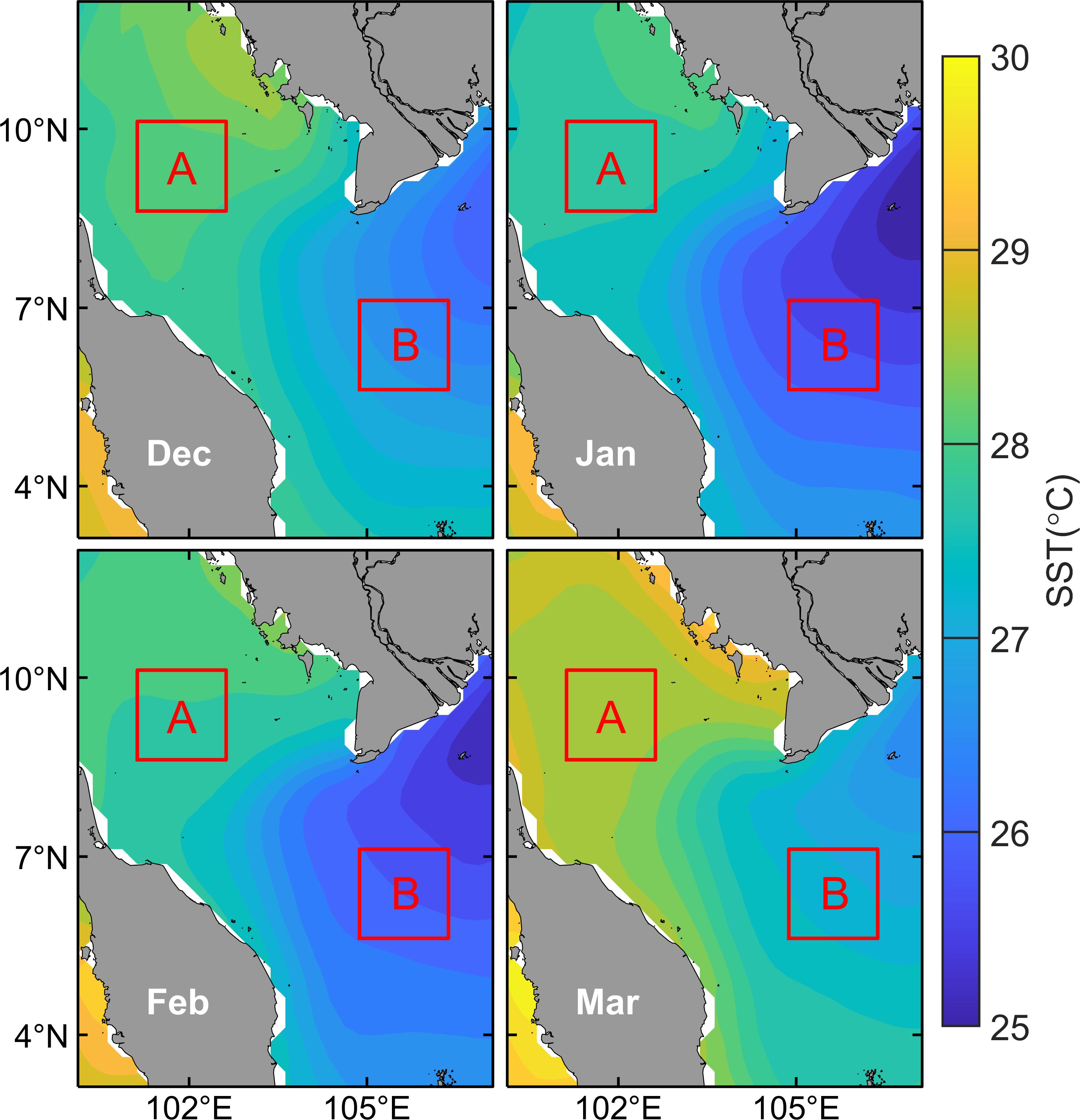
Figure 10 Monthly variation of SST from December to March (°C, shading). The box A and box B with red bold contour line represent the west and east sea area of the TFEGT, respectively.

Figure 11

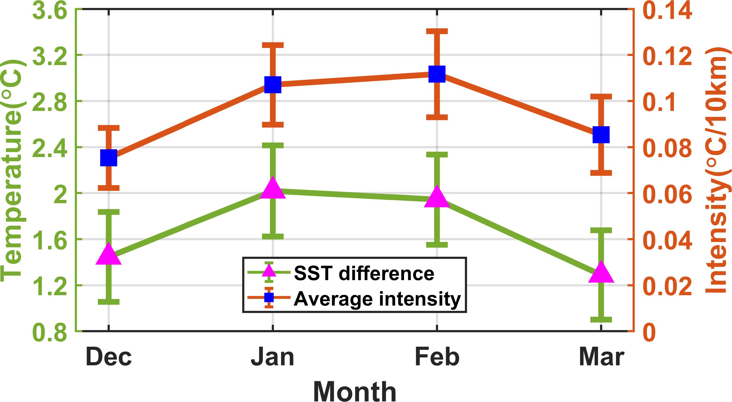
Figure 11 Monthly variation of SST difference (°C, in blue) between two sides of the TFEGT and intensity (°C/10 km, in orange) of the thermal front with their standard deviations from December to March.

Figure 12

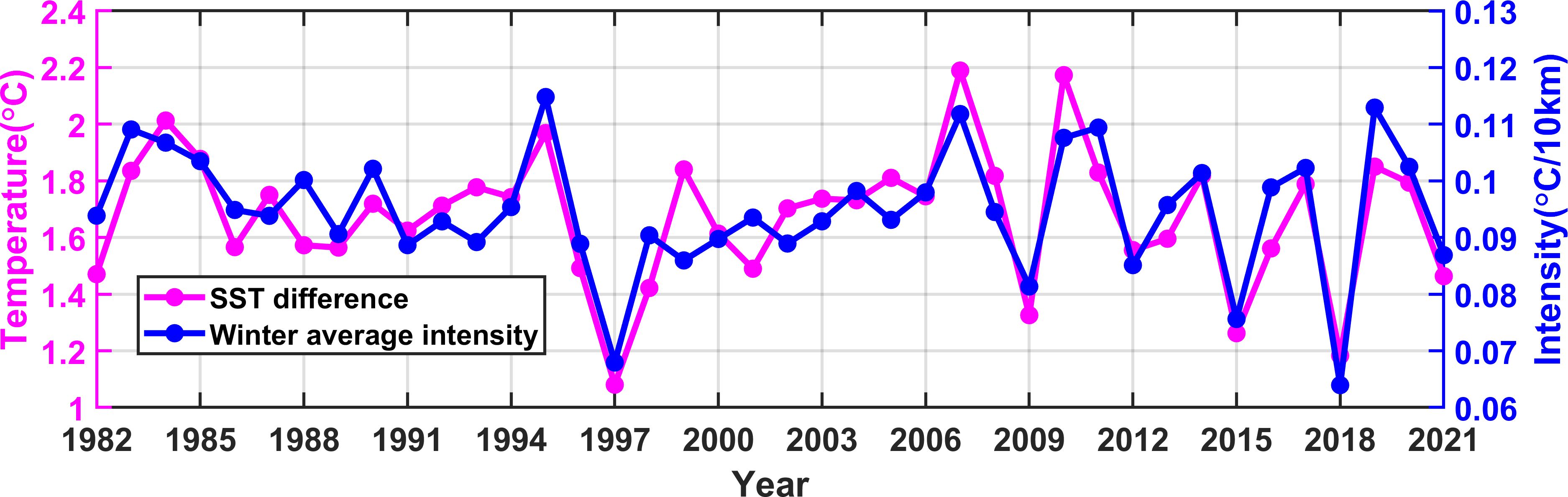
Figure 12 The time series of annual SST difference (°C, in blue) between two sides of the TFEGT and intensity (°C/10 km, in orange) of the thermal front in winter from 1982 to 2021.

The SST variation can be assessed by the mixed layer temperature equation (Qu, 2001; Wang and Wang, 2006; Qiu et al., 2015). The contributions of the net surface heat flux term, Ekman heat advection term, geostrophic heat advection term, and vertical heat entrainment term are shown in Figure 13. The vertical heat entrainment term exhibits a minimal impact, whereas net surface heat flux term and geostrophic heat advection term play significant roles. Figure 14 provides the contributions difference of the five terms in the temperature equation between the two sides of the TFEGT. The Ekman heat advection term and vertical heat entrainment term are generally small; thus, they exert little influence on spatial distribution of SST around the GoT. The other two terms play opposite roles and their impact primarily concentrated on the surface of the sea outside GoT. The net surface heat flux (geostrophic heat advection) induces a positive (negative) SST change about 0.5°C–1.5°C/month (0.5°C–2°C/month). In contrast to the SST trend term, the spatial distribution of SST in the GoT, featuring lower temperatures in the east and higher temperature in the west, is consistent with the pattern of geostrophic heat advection term and opposite to the pattern of the net surface heat flux term. Hence, the geostrophic flow is the primary factor leading to the spatial distribution pattern of SST in the GoT. Figure 13C shows that the geostrophic current flows along the east coast of Vietnam into GoT, proceeds southward at the mouth of the gulf, and then continues its southward flow along the Malay Peninsula. It suggests that the southward transport of cold water from the northern SCS is the key contributing to the formation of the TFEGT.

Figure 13

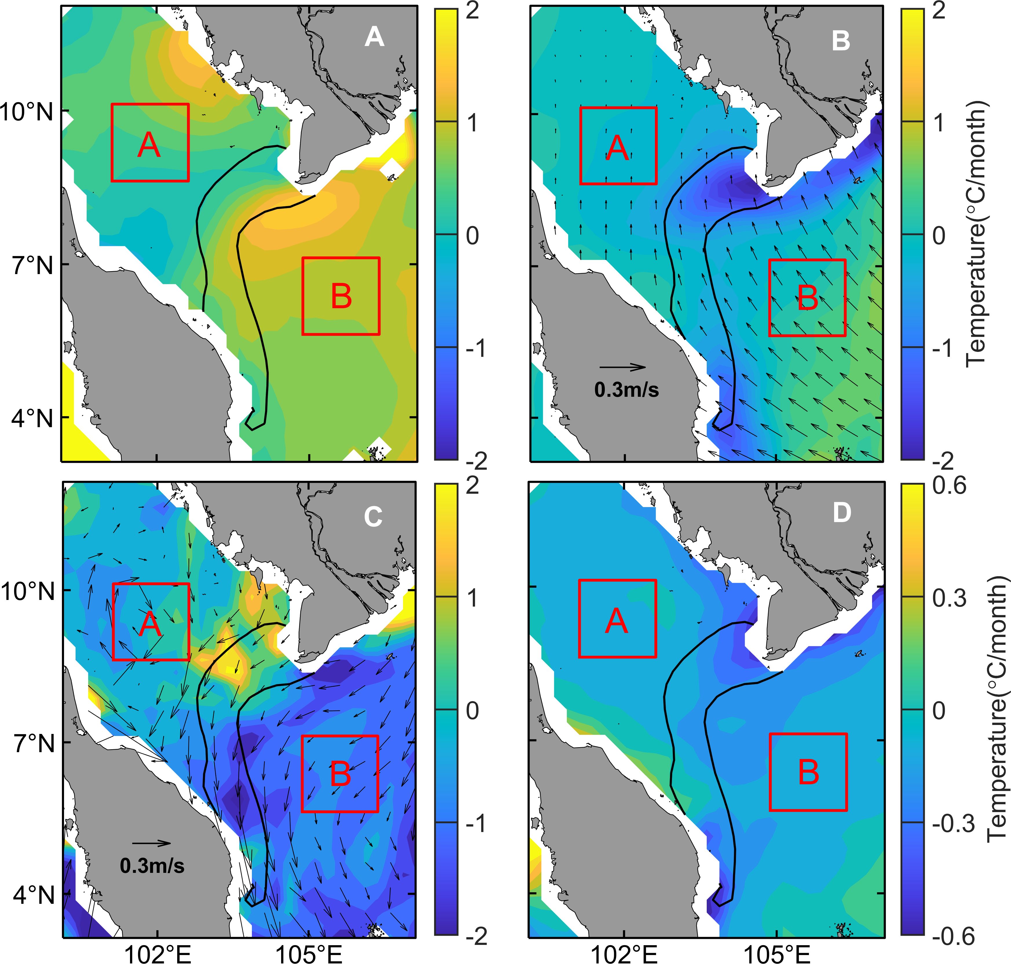
Figure 13 (A) Net surface heat flux term. (B) Ekman thermal advection term with surface Ekman velocity. (C) Geostrophic heat advection term with surface geostrophic velocity. (D) Vertical entrainment term. Unit: °C/month. Each item is the average of the climate state. The definitions of the box A and box B are consistent with that in Figure 10. The definition of the black solid lines is consistent with that in Figure 1B.

Figure 14

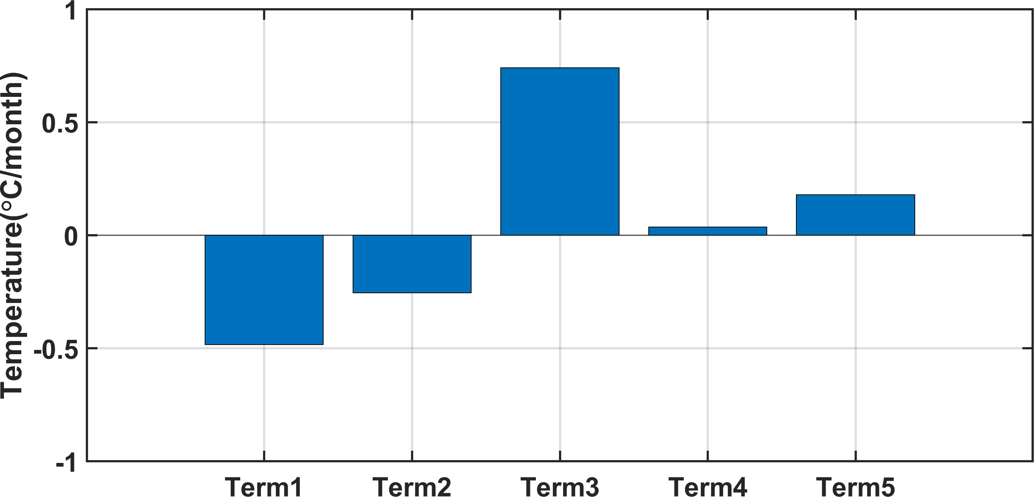
Figure 14 Terms 1–5 represent the SST difference (°C/month) of the net surface heat flux term, Ekman thermal advection term, geostrophic heat advection term, vertical entrainment term, and SST tendency term, respectively.

The ocean circulation pattern of the SCS is mainly controlled by wind stress curl (Wu et al., 1998; Shaw et al., 1999). In winter, the sustained negative wind stress curl in the northern SCS and northeast monsoon jointly modulate the intensity of the western boundary current from northern Vietnam to the southern coast (Amedo and Villanoy, 2003; Lian et al., 2015; Kuo and Tseng, 2020).

According to the analysis in Section 3.2, the interannual variation of TFEGT is related with the ENSO. We respectively composite the SST, geostrophic current, and wind of winter climatology in the Figures 15A, D, strong El Niño years in the Figures 15B, E and in strong La Niña years in the Figures 15C, F. In strong El Niño years, the northeast monsoon wind speed across the entire SCS is comparatively low, leading to a decrease in the velocity of the western boundary current and a reduction in the southward transport of cold water from the north. The temperature of the seawater reaching the GoT is higher than the climatology, so the temperature difference with the seawater inside the gulf is smaller, resulting in a weaker thermal front. Conversely, in strong La Niña years, the northeast monsoon over the SCS is strong and the wind speed is high, strengthening the flow velocity of the western boundary current. The cold water in the north is transported in large quantities to the south, and the temperature of the seawater reaching the GoT is lower compared with the climatology. The temperature difference between the seawater at the mouth of GoT and the seawater inside the gulf is relatively large, contributing to the intensification of the thermal front.

Figure 15

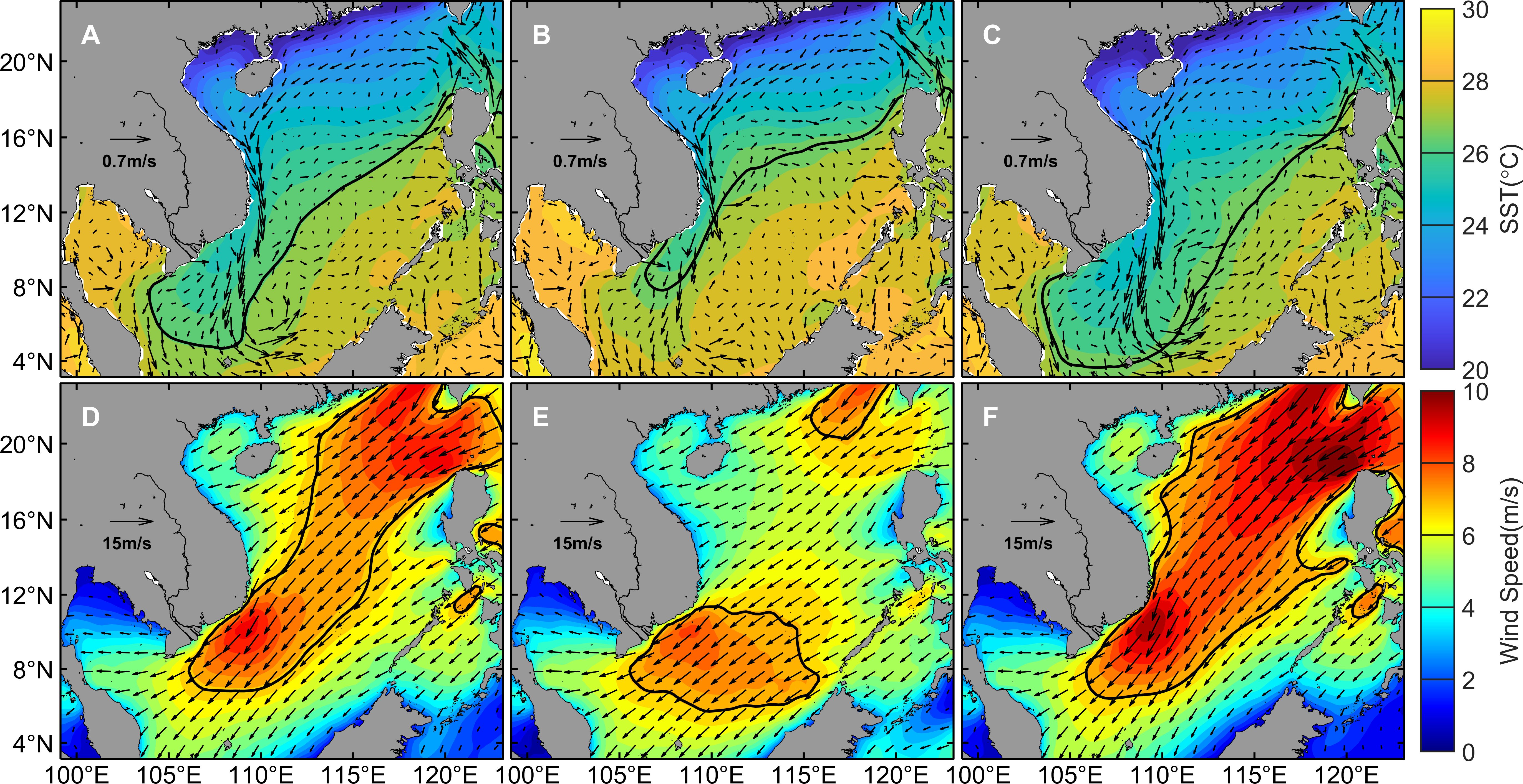
Figure 15 (A) Winter climatology SST (°C, in color, the black line is 26.8°C contour line) with geostrophic current (m/s, in vector). (B) Winter SST with geostrophic current in strong El Niño year. (C) Winter SST with geostrophic current in strong La Niña year. (D) Winter climatology wind speed (m/s, in color, the black line is 7 m/s contour line) with wind vector (m/s, in vector). (E) Winter wind speed with wind vector in strong El Niño years. (F) Winter wind speed with wind vector in strong La Niña year.

4 Conclusion

Based on a series of satellite observation data and reanalysis data, we studied the TFEGT during the winter from 1982 to 2021. The TFEGT has notable seasonal variation. In December, the probability of the front occurrence stands at approximately 40%, accompanied by smaller intensity and area. The area and intensity of the thermal front attain their maximum values and most pronounced in January and February, with the probability of the front occurrence reaching 70%–80%. In March, all the three indicators experience a substantial decrease. The interannual variability of the TFEGT is also evident, characterized by being strong in 1983, 1984, 1995, 2007, 2010, 2011, and 2019 and being weak in 1997, 2009, 2015, and 2018, which is related with ENSO. The greatest impact of ENSO on the TFEGT occurs 2 months prior to the front’s formation, with the correlation coefficient between the Niño3 index and the intensity of the TFEGT of −0.58. The specific adjustment process is as follows. In the strong El Niño (La Niña) year, the northeast monsoon weakens (strengthens), causing a weakening (strengthening) of the western boundary current in the SCS. Then, the cold water flow entering the GoT exhibits a higher (lower) temperature, inducing a weaker (stronger) thermal front.

Then, we use the mixed layer temperature equation to delve into the formation mechanism of the TFEGT. The geostrophic heat advection emerges as a pivotal factor in the formation of TFEGT. In winter, the prevailing northeast monsoon drives a southward movement of the western boundary current along the coast of Vietnam, which transports cold water from the north to the south. This further propels the decline of SST east of GoT and expands the SST difference in the mouth of GoT, ultimately resulting in the formation of the TFEGT.

Although this paper found a robust connection between the interannual variation of the TFEGT and ENSO, the abnormal enhancements or weakening of the thermal fronts have been observed in certain years when El Niño or La Niña phenomena have not occurred. This prompts the need for more exploration and research on climate. In addition, the Mekong River water mass may have some impact on the formation of TFEGT, we will collect the relevant hydrological data for further analysis.

Data availability statement

The original contributions presented in the study are included in the article/supplementary material. Further inquiries can be directed to the corresponding author.

Author contributions

LZ: Formal analysis, Validation, Visualization, Writing – original draft. RS: Data curation, Investigation, Writing – review & editing. PL: Resources, Supervision, Writing – review & editing. GY: Writing – review & editing.

Funding

The author(s) declare financial support was received for the research, authorship, and/or publication of this article. This study was supported by the Hainan Provincial Joint Project of Sanya Yazhou Bay Science and Technology City under contract no. 2021CXLH0020, the Project of Sanya Yazhou Bay Science and Technology City under contract no. SCKJ-JYRC-2022–47, and the Natural Science Foundation of Hainan Province under contract no. 121MS062.

Conflict of interest

The authors declare that the research was conducted in the absence of any commercial or financial relationships that could be construed as a potential conflict of interest.

Publisher’s note

All claims expressed in this article are solely those of the authors and do not necessarily represent those of their affiliated organizations, or those of the publisher, the editors and the reviewers. Any product that may be evaluated in this article, or claim that may be made by its manufacturer, is not guaranteed or endorsed by the publisher.

References

Amedo C. L., Villanoy C. (2003). Wind stress curl and surface circulation in the south China sea and the philippine sea. Sci. Diliman 15, (2).

Google Scholar

Aschariyaphotha N., Wongwises P., Wongwises S., Humphries U. W., You X. (2008). Simulation of seasonal circulations and thermohaline variabilities in the Gulf of Thailand. Adv. Atmospheric Sci. 25, 489–506. doi: 10.1007/s00376-008-0489-3

CrossRef Full Text | Google Scholar

Atlas R., Hoffman R. N., Ardizzone J., Leidner S. M., Jusem J. C., Smith D. K., et al. (2011). A cross-calibrated, multiplatform ocean surface wind velocity product for meteorological and oceanographic applications. Bull. Am. Meteorological Soc. 92, 157–15+. doi: 10.1175/2010BAMS2946.1

CrossRef Full Text | Google Scholar

Belkin I., Cornillon P. (2003). SST fronts of the Pacific coastal and marginal seas. Pacific Oceanography 1, 90–113.

Google Scholar

Belkin I. M., Cornillon P. C., Sherman K. (2009). Fronts in large marine ecosystems. Prog. Oceanography 81, 223–236. doi: 10.1016/j.pocean.2009.04.015

CrossRef Full Text | Google Scholar

Buranapratheprat A., Yanagi T., Sawangwong P. (2002). Seasonal variations in circulation and salinity distributions in the upper Gulf of Thailand: Modeling approach. Mer (Tokyo) 40, 147–155.

Google Scholar

Carton J. A., Chepurin G. A., Chen L. (2018). SODA3: A new ocean climate reanalysis. J. Climate 31, 6967–6983. doi: 10.1175/JCLI-D-18-0149.1

CrossRef Full Text | Google Scholar

Carton J. A., Giese B. S. (2005). SODA: A reanalysis of ocean climate. J. Geophysical Research-Oceans. Available at: https://www2.atmos.umd.edu/~carton/pdfs/carton&giese05.pdf.

Google Scholar

Carton J. A., Giese B. S. (2008). A reanalysis of ocean climate using Simple Ocean Data Assimilation (SODA). Monthly Weather Rev. 136, 2999–3017. doi: 10.1175/2007MWR1978.1

CrossRef Full Text | Google Scholar

Chang Y., Shieh W. J., Lee M. A., Chan J. W., Lan K. W., Weng J. S. (2010). Fine-scale sea surface temperature fronts in wintertime in the northern South China Sea. Int. J. Remote Sens. 31, 4807–4818. doi: 10.1080/01431161.2010.485146

CrossRef Full Text | Google Scholar

Chelton D. B., Schlax M. G., Samelson R. M. (2007). Summertime coupling between sea surface temperature and wind stress in the California Current System. J. Phys. Oceanography 37, 495–517. doi: 10.1175/JPO3025.1

CrossRef Full Text | Google Scholar

Chu P. C., Edmons N. L., Fan C. W. (1999). Dynamical mechanisms for the South China Sea seasonal circulation and thermohaline variabilities. J. Phys. Oceanography 29, 2971–2989. doi: 10.1175/1520-0485(1999)029<2971:DMFTSC>2.0.CO;2

CrossRef Full Text | Google Scholar

Fang G., Chen H., Wei Z., Wang Y., Wang X., Li C. (2006). Trends and interannual variability of the SCS surface winds, surface height, and surface temperature in the recent decade. J. Geophysical Research-Oceans 111, C11S16. doi: 10.1029/2005JC003276

CrossRef Full Text | Google Scholar

Gao S., Wang H. (2008). Seasonal and spatial distributions of phytoplankton biomass associated with monsoon and oceanic environments in the South China Sea. Acta Oceanol. Sin. 27, 17–32.

Google Scholar

Hu J., Kawamura H., Hong H., Qi Y. (2000). A review on the currents in the south China sea: seasonal circulation, south China sea warm current and kuroshio intrusion. J. Oceanography 56, 607–624. doi: 10.1023/A:1011117531252

CrossRef Full Text | Google Scholar

Huang B., Liu C., Banzon V., Freeman E., Graham G., Hankins B., et al. (2021). Improvements of the daily optimum interpolation sea surface temperature (DOISST) version 2.1. J. Climate 34, 2923–2939. doi: 10.1175/JCLI-D-20-0166.1

CrossRef Full Text | Google Scholar

Jackett D. R., McDougall T. J., Feistel R., Wright D. G., Griffies S. M. (2006). Algorithms for density, potential temperature, conservative temperature, and the freezing temperature of seawater. J. Atmospheric Oceanic Technol. 23, 1709–1728. doi: 10.1175/JTECH1946.1

CrossRef Full Text | Google Scholar

Kuo Y.-C., Tseng Y.-H. (2020). Impact of ENSO on the South China Sea during ENSO decaying winter–spring modeled by a regional coupled model (a new mesoscale perspective). Ocean Model. 152, 101655. doi: 10.1016/j.ocemod.2020.101655

CrossRef Full Text | Google Scholar

Li C. Y., Hu J. Y., Jan S., Wei Z. X., Fang G. H., Zheng Q. N. (2006). Winter-spring fronts in Taiwan strait. J. Geophysical Research-Oceans 111, C11S13. doi: 10.1029/2005JC003203

CrossRef Full Text | Google Scholar

Li J., Zhang R., Ling Z., Bo W., Liu Y. (2014). Effects of Cardamom Mountains on the formation of the winter warm pool in the gulf of Thailand. Continental Shelf Res. 91, 211–219. doi: 10.1016/j.csr.2014.10.001

CrossRef Full Text | Google Scholar

Lian Z., Fang G., Wei Z., Wang G., Sun B., Zhu Y. (2015). A comparison of wind stress datasets for the South China Sea. Ocean Dynamics 65, 721–734. doi: 10.1007/s10236-015-0832-z

CrossRef Full Text | Google Scholar

Liu Q., Kaneko A., Su J. (2008). Recent progress in studies of the South China Sea circulation. J. Oceanography 64, 753–762. doi: 10.1007/s10872-008-0063-8

CrossRef Full Text | Google Scholar

Locarnini R. A., Mishonov A. V., Baranova O. K., Boyer T. P., Zweng M. M., Garcia H. E., et al. (2018). World ocean atlas 2018, volume 1: temperature (A. Mishonov Technical Ed. NOAA Atlas NESDIS), 81, 52pp.

Google Scholar

Mears C. A., Scott J., Wentz F. J., Ricciardulli L., Leidner S. M., Hoffman R., et al. (2019). A near-real-time version of the cross-calibrated multiplatform (CCMP) ocean surface wind velocity data set. J. Geophysical Research-Oceans 124, 6997–7010. doi: 10.1029/2019JC015367

CrossRef Full Text | Google Scholar

Penyapol A. (1957). Report on oceanographic surveys carried out in the Gulf of Thailand during the years 1956–1957. Bangkok: Hydrography Depth Royal, Thai Navy, 12.

Google Scholar

Pi Q. L., Hu J. Y. (2010). Analysis of sea surface temperature fronts in the Taiwan Strait and its adjacent area using an advanced edge detection method. Sci. China-Earth Sci. 53, 1008–1016. doi: 10.1007/s11430-010-3060-x

CrossRef Full Text | Google Scholar

Pujol M. (2022). Product user manual for sea level SLA products (Copernicus Monitoring Environment Marine Service (CMEMS). Available at: https://catalogue.marine.copernicus.eu/documents/PUM/CMEMS-SL-PUM-008–032-068.pdf.

Google Scholar

Qiu C. H., Mao H. B., Yu J. C., Xie Q., Wu J. X., Lian S. M., et al. (2015). Sea surface cooling in the Northern South China Sea observed using Chinese sea-wing underwater glider measurements. Deep-Sea Res. Part I-Oceanographic Res. Papers 105, 111–118. doi: 10.1016/j.dsr.2015.08.009

CrossRef Full Text | Google Scholar

Qu T. D. (2000). Upper-layer circulation in the south China sea. J. Phys. Oceanography 30, 1450–1460. doi: 10.1175/1520-0485(2000)030<1450:ULCITS>2.0.CO;2

CrossRef Full Text | Google Scholar

Qu T. D. (2001). Role of ocean dynamics in determining the mean seasonal cycle of the South China Sea surface temperature. J. Geophysical Research-Oceans 106, 6943–6955. doi: 10.1029/2000JC000479

CrossRef Full Text | Google Scholar

Qu T., Du Y., Gan J., Wang D. (2007). Mean seasonal cycle of isothermal depth in the South China Sea. J. Geophysical Research-Oceans 112, C02020. doi: 10.1029/2006JC003583

CrossRef Full Text | Google Scholar

Reynolds R. W., Smith T. M., Liu C., Chelton D. B., Casey K. S., Schlax M. G. (2007). Daily high-resolution-blended analyses for sea surface temperature. J. Climate 20, 5473–5496. doi: 10.1175/2007JCLI1824.1

CrossRef Full Text | Google Scholar

Shaw P.-T., Chao S.-Y., Fu L.-L. (1999). Sea surface height variations in the South China Sea from satellite altimetry. Oceanologica Acta 22, 1–17. doi: 10.1016/S0399-1784(99)80028-0

CrossRef Full Text | Google Scholar

Snidvongs A. (1998). The oceanography of the Gulf of Thailand: Research and management policy. SEAPOL integrated Stud. Gulf Thailand 1, 1–68.

Google Scholar

Sun R., Ling Z., Chen C., Yan Y. (2015). Interannual variability of thermal front west of Luzon Island in boreal winter. Acta Oceanol. Sin. 34, 102–108. doi: 10.1007/s13131-015-0753-1

CrossRef Full Text | Google Scholar

Tang D. L., Kawamura H., Shi P., Takahashi W., Guan L., Shimada T., et al. (2006). Seasonal phytoplankton blooms associated with monsoonal influences and coastal environments in the sea areas either side of the IndoChina Peninsula. J. Geophysical Research-Biogeosciences 111, G01010. doi: 10.1029/2005JG000050

CrossRef Full Text | Google Scholar

Ullman D. S., Cornillon P. C. (1999). Satellite-derived sea surface temperature fronts on the continental shelf off the northeast US coast. J. Geophysical Research-Oceans 104, 23459–23478. doi: 10.1029/1999JC900133

CrossRef Full Text | Google Scholar

Wang G., Li J., Wang C., Yan Y. (2012). Interactions among the winter monsoon, ocean eddy and ocean thermal front in the South China Sea. J. Geophysical Research-Oceans 117, C08002. doi: 10.1029/2012JC008007

CrossRef Full Text | Google Scholar

Wang W. Q., Wang C. Z. (2006). Formation and decay of the spring warm pool in the South China Sea. Geophysical Res. Lett. 33, L02615. doi: 10.1029/2005GL025097

CrossRef Full Text | Google Scholar

Wang C. Z., Wang W. Q., Wang D. X., Wang Q. (2006). Interannual variability of the SCS associated with El Nino. J. Geophysical Research-Oceans 111, C03023. doi: 10.1029/2005jc003333

CrossRef Full Text | Google Scholar

Wang Y., Yu Y., Zhang Y., Zhang H. R., Chai F. (2020). Distribution and variability of sea surface temperature fronts in the south China sea. Estuar. Coast. Shelf Sci. 240, 106793. doi: 10.1016/j.ecss.2020.106793

CrossRef Full Text | Google Scholar

Wentz F. J., Scott J., Hoffman R., Leidner M., Atlas R., Ardizzone J. (2015). Remote Sensing Systems Cross-Calibrated Multi-Platform (CCMP) 6-hourly ocean vector wind analysis product on 0.25 deg grid, Version 2.0 (Santa Rosa, CA: Remote Sensing Systems). Available at: www.remss.com/measurements/ccmp.

Google Scholar

Woodson C. B., Litvin S. Y. (2015). Ocean fronts drive marine fishery production and biogeochemical cycling. Proc. Natl. Acad. Sci. United States America 112, 1710–1715. doi: 10.1073/pnas.1417143112

CrossRef Full Text | Google Scholar

Wu C. R., Shaw P. T., Chao S. Y. (1998). Seasonal and interannual variations in the velocity field of the South China Sea. J. Oceanogr 54, 361–372. doi: 10.1007/BF02742620

CrossRef Full Text | Google Scholar

Wyrtki K. (1961). Scientific results of marine investigations of the South China Sea and the Gulf of Thailand 1959–1961. NAGA Rep. 2, 195.

Google Scholar

Xue H. J., Chai F., Pettigrew N., Xu D. Y., Shi M., Xu J. P. (2004). Kuroshio intrusion and the circulation in the South China Sea. J. Geophysical Research-Oceans 109, C02017. doi: 10.1029/2002JC001724

CrossRef Full Text | Google Scholar

Yanagi T., Takao T. (1998). Seasonal variation of three-dimensional circulations in the Gulf of Thailand. La mer 36, 43–55.

Google Scholar

Yu Y., Zhang H.-R., Jin J., Wang Y. (2019). Trends of sea surface temperature and sea surface temperature fronts in the South China Sea during 2003–2017. Acta Oceanol. Sin. 38, 106–115. doi: 10.1007/s13131-019-1416-4

CrossRef Full Text | Google Scholar

Zhu F., Xie L., Cheng Y. (2014). Distribution and seasonal variation of temperature fronts in the South China Sea. Oceanologia Limnologia Sin. 45, 695–702. doi: 10.11693/hyhz20130600075

CrossRef Full Text | Google Scholar