The Black Sea near-past wave climate and its variability: a hindcast study

This study analyzed the past wave climate of the Black Sea region for the period from 1988 to 2021. The wave field has been simulated using the state-of-the-art, third-generation wave model WAVEWATCH III forced by the ECMWF reanalysis ERA5 winds, with the model resolution being the highest ever applied to the region in a basin-scale climate study. The surface currents provided by the Copernicus Marine Service have been included in the wave model to evaluate wave–current interactions. The wave model results have been validated with respect to satellite and buoy observations, showing that the simulation accurately reproduces the past evolution of the wave field, exceeding 0.9 correlation with respect to satellite data. The inclusion of wave–current interaction has been positively evaluated. Four statistics (significant wave height 5th and 95th percentiles, mean, and maxima) have been used to describe the wave field at seasonal timescale, showing a clear distinction between the Western (rougher sea conditions) and Eastern (calmer sea conditions) sub-basins. Furthermore, the intra-annual wave climate variability has been investigated using a Principal Component Analysis (PCA) and the Mann–Kendall test on significant wave height (SWH). This study represents the first time the PCA is applied to the region, identifying two main modes that highlight distinct features and seasonal trends in the Western and Eastern sub-basins. Throughout most seasons, the SWH trend is positive for the Eastern basin and negative for the Western basin. The PCA shows a regime shift with increasing eastward waves and decreasing north and north-eastward waves. Finally, SWH correlation (ρ) with four Teleconnection indexes (East Atlantic Pattern, Scandinavian Pattern, North Atlantic Oscillation, and East Atlantic/West Russia Pattern) revealed that the strongest ρ is observed with the Eastern–Atlantic–Western Russia teleconnection, with a peculiar spatial pattern of correlation, and is positive for the northwestern and negative for the southeastern sub-basin.

1 Introduction

Studying the wave climate of a region is crucial for various socio-economic activities such as shipping, coastal infrastructure planning, and environmental conservation efforts. In recent years, advancements in numerical modeling techniques coupled with high-resolution atmospheric data have provided valuable insights into the complex dynamics of ocean waves.

It is well known that the performance of wave models depends heavily on the quality and resolution of the driving wind fields (Holthuijsen et al., 1996; Cavaleri and Bertotti, 2006; Ardhuin et al., 2007). According to Cavaleri and Bertotti (2006) and Cavaleri et al. (2024), modeling wind and waves is less precise in enclosed basins compared to open-ocean conditions, primarily because the presence of land significantly affects the marine surface wind fields. For this reason, climate studies are revised when computational capabilities permit enhancements in spatial resolution for both atmospheric and wave models, as well as longer temporal integration.

The Black Sea (hereinafter referred to as BS) is an inland sea, situated as the easternmost extension of the Atlantic Ocean basin, spanning latitudes between 41 and 46°N and longitudes 27 and 42°E. It is linked to the Mediterranean Sea via the Sea of Marmara and the Bosphorus and Dardanelles straits in the southwest and connects to the Sea of Azov through the Kerch Strait in the northeast. A peculiarity of the BS is the steep continental slope and the exceptionally narrow continental shelf—except in the northwestern and western regions. The majority of the sea comprises a basin with a relatively flat bottom relief and depths exceeding 2,000 m (Arkhipkin et al., 2014). A significant portion of the BS’s coastline is bordered by mountains such as the Balkans, Pontic Mountains, Caucasus, and Crimean Mountains. This geographical feature contributes to distinct wind patterns in the coastal regions of the sea. Further details about the entire BS system can be found in Özsoy and Ünlüata (1997) and Kostianoy (2008).

Wind waves in the BS have been studied by several authors in the last decades. Most of the work aimed to describe temporal mid-term wave field, generally less than 15 years (Divinsky and Kos’ yan, 2015; Divinsky and Kosyan, 2018) or the sub-regional part of the basin, as in Rusu (2019) and Akcay et al. (2022). Recently, there is a growing interest in the investigation of future projections, as in the studies of Islek et al. (2022) and Çakmak et al. (2023), which presented wave climate projections for the mid and the end of the century.

From a modeling perspective, the most used numerical models for the BS region are the SWAN model (Booij et al., 1999; Ris et al., 1999; Holthuijsen et al., 2001; Rusu et al., 2014; Rusu, 2019; Islek et al., 2022; Rybalko and Myslenkov, 2022) and MIKE 21 (Warren and Bach, 1992; Divinsky and Kos’ yan, 2015; Divinsky and Kosyan, 2017, 2018; Divinsky et al., 2020). Only recently (Causio et al., 2021; Soran et al., 2022) has the state-of the-art WAVEWATCHIII wave model (hereafter WW3) been adopted in the Black Sea and still very few studies exploited the last atmospheric reanalysis ERA5 from ECMWF (Çalışır et al., 2023; Acar et al., 2023).

The aim of the present study is to comprehensively describe the BS wave climate and its variability during the time period 1988–2021. The WW3 wave model used in this study has been forced by the ECMWF-ERA5 reanalysis and implemented at a high horizontal resolution (~3 km), marking the highest resolution adopted in a comprehensive climatology study within the BS regional domain. Therefore, from a modeling perspective, this work represents the first instance of simulating the BS wave climate with WW3 and ERA5, introducing an unprecedented horizontal resolution for a climate study of the basin as a whole. It is noteworthy to mention that while other studies have utilized higher resolutions, these were typically applied for shorter time scales or confined to sub-regional domains (Akpınar et al., 2012; Rusu, 2019). Furthermore, the work represented the opportunity to assess and include the wave–current interaction in the model physics.

The description of the wave climate includes a thorough examination ranging from fundamental statistical description to the investigation of intra-annual and inter-annual variability. Four statistical descriptors have been used for characterizing the seasonal and geographic distribution of significant wave height (SWH): mean, maximum, and 5th and 95th percentiles, and we proposed a methodology in associating wave direction to each statistic. Furthermore, the climate variability has been analyzed by applying the Mann–Kendall test and, for the first time in the BS region, by employing the Principal Component Analysis. In conclusion, the study aims to establish the correlation between the wave climate and the main atmospheric teleconnections. The correlation between Teleconnection indices (TLC) and BS waves has been investigated by Saprykina et al. (2019), but for a different time period 1955–2007 and different wave data [visual wave observations (Voluntary Observing Ship) and WAM wave modeling (Günther et al., 1992) forced by NCEP wind reanalysis (Kalnay, 1996)].

By addressing all these various aspects, our goal is to present a holistic and detailed understanding of the Black Sea wave climate, capturing its features and relationships.

The article is organized as follows: Section 2, Material and methods, describes the wave model and the modeling setup, the forcing datasets, the observing datasets, and the numerical experiments. Section 3, Results and discussion, details the model validation and the description of the wave climate from 1988 to 2021, distinguishing intra-annual variability from inter-annual variability, trends, and correlations between SWH and TLC patterns. The last section, 4, Conclusion, summarizes the main outcomes of the work.

2 Materials and methods

2.1 Wave modeling setup

The wave numerical core adopted in the Black Sea simulations is the third-generation spectral WAVEWATCH III model version 6.07 (Tolman, 2009; WW3DG, 2019). The model solves the random phase action density balance equation for wavenumber-direction spectra.

In this study, the WW3 configuration at approximately 3 km of horizontal resolution was based on previous studies. The horizontal domain discretization and related bathymetric dataset are derived from Ciliberti et al. (Ciliberti et al., 2021, 2022) and represent a consolidated benchmark used also in Causio et al. (2021).

The final configuration of the model was obtained by calibration through multiple sensitivity tests. The methodological approach we adopted in its definition is summarized in Figure 1. The objective of the calibration aimed to improve the model accuracy and to reduce the observed underestimation of the wave height emerged during the sensitivity tests, when ECMWF-ERA5 winds were used. The ERA5 underestimation, particularly for high wind, has been even recently documented by Çalışır et al. (2023). The first step of the implementation, the definition of spectral and horizontal discretization, time stepping, and propagation scheme, was based on the previous study by Causio et al. (2021). Afterwards, considering that this study employed a different atmospheric forcing with respect to the previous study (with lower spatial resolution and higher temporal frequency), sensitivity experiments were performed aiming to tune the input and dissipation source term. We assessed all the model physics available in WW3, finding that ST4 physics based on Ardhuin et al. (2010) provided the best skills. The Discrete Interaction Approximation for non-linear wave–wave interaction, bottom friction based on JONSWAP (Hasselmann et al., 1973), and depth-induced breaking based on the work of Battjes and Janssen (1978) contributed in improving the model performance. Furthermore, we found that a specific calibration of the wind-wave coupling parameter (BETAMAX), wind-gustiness parameter (ZALP), and the cumulative breaking term (SDSCUM) helped in enhancing the model results limiting the underestimation of the wave height. According to previous studies (Alday et al., 2021; Mentaschi et al., 2023) conducted on a global scale, the parameter BETAMAX should be set to a higher value compared to ours when utilizing ERA5 atmospheric forcings. However, our calibration experiments revealed an overestimation of high waves with this setting. Conversely, employing ZALP aided in reducing negative bias without causing an overshoot in high waves. This varying sensitivity of the model to BETAMAX could reasonably be attributed to the smaller size of the domain, which, in our case, pertains to a small regional area.

Figure 1

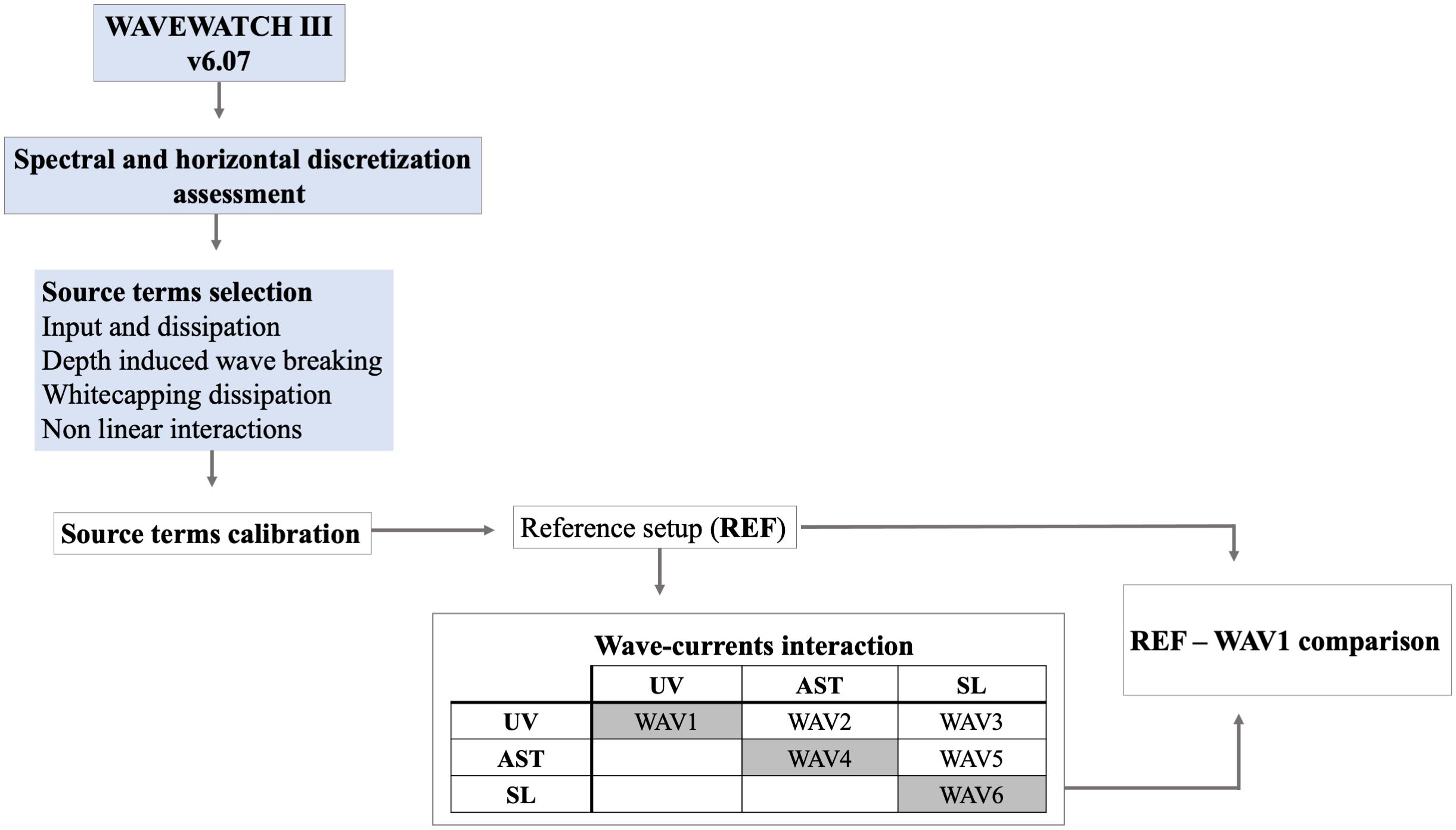
Figure 1 Model implementation steps. Light blue text box refers to the implementation inherited by Causio et al. (2021). White filled text boxes indicated the implementation steps performed in this work. The wave–currents interaction table details the tested configurations. UV, current forcing; AST, air–sea temperature difference forcing; SL, sea-level forcing. Gray cells indicated the usage of only one hydrodynamic forcing in addition to the REF configuration.

Despite the fact that the implementation/calibration phase represented the foundation of the model, this study focused on the wave climate assessment of the BS; thus, we did not include a dedicated discussion here. However, more details about the final configurations are provided in Table 1.

Table 1

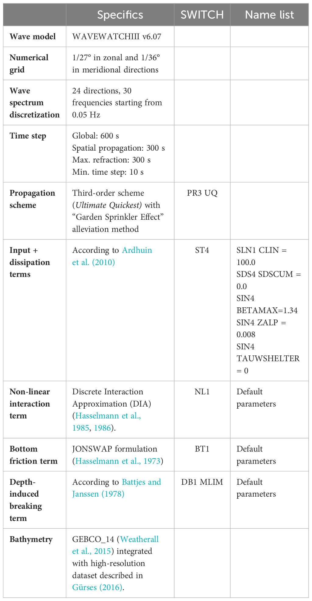
Table 1 WW3 model configuration and physics adopted in this work.

Moreover, this work represented the opportunity to investigate if the oceanic field forcings affect the BS wave climate. The final configuration obtained by the aforementioned sensitivity tests represented our reference setup (hereafter REF), namely, the model implementation with the highest performances without hydrodynamic forcings. Only after configuring the REF implementation did we proceed to include hydrodynamic fields to identify their effects, without changing any of the REF parameters.

WW3 can be forced by three different hydrodynamical fields: sea level, currents, and air–sea temperature difference (more details are provided in Causio et al., 2021). All the possible combinations have been tested, and only current forcing induced a valuable positive effect on the wave field. In contrast, with the other combinations, we obtained no significant changes or worse skills. Taking this into consideration, the statistical analysis was based only on the reference (hereafter REF, control experiment without hydrodynamic forcing) and the current-forced experiments (hereafter WAV1), omitting redundant and less informative results.

2.2 The forcing data

In this study, the wave model has been forced by the most recent reanalysis winds from the European Centre for Medium-range Weather Forecasts (ECMWF), ERA5 (Hersbach et al., 2020) (Figure 3A). ERA5 supersedes the ERA-Interim reanalysis and is the fifth-generation ECMWF reanalysis for global climate and weather for the past seven decades. ERA5 provides hourly estimates for atmospheric variables on a regular latitude–longitude grid of 0.25°.

The Copernicus Marine Service (hereafter CMS) (https://marine.copernicus.eu/it) is a European provider of ocean data for the Black Sea, European Seas, and the global ocean. The CMS BLKSEA_MULTIYEAR_PHY_007_004 product (BLKMY)¹ (Lima et al., 2021; BS-PHY_REA) provides monthly and daily hydrodynamic fields for the BS basin. In this work, we used daily sea-surface temperature, sea level, and currents (Figure 3B). The hydrodynamical core of the product is based on NEMO general circulation ocean model v3.6, tailored to the BS domain with a horizontal resolution of 1/27° × 1/36° and 31 vertical levels. The ocean model is forced by the atmospheric reanalysis ECMWF ERA5 at 1 h in frequency. The model assimilates CMS sea-level anomaly along-track observations and in situ vertical profiles of temperature and salinity from both SeaDataNet and CMS datasets, using the OceanVar (Dobricic and Pinardi, 2008; Storto et al., 2011).

2.3 The wave observational datasets

The BS region has scarce measured data, particularly for waves. Two main CMS datasets have been used during calibration and validation of the wave model:

I. Satellite data, WAVE_GLO_PHY_SWH_L3_NRT_ 393 014_001² (Wave_L3_NRT)

II. Mooring data, INSITU_BLK_PHYBGCWAV 395 _DISCRETE_MYNRT_013_034³ (BS_INS_NRT)

At the time of this study, satellite-based along-track SWH was available in CMS from July 2019 to December 2021. The dataset incorporates multiple satellite missions: Cryosat-2, AltiKa, HY-2B, Jason-3, Sentinel-3A, and Sentinel-3B on which a systematic quality control is applied, combining various criteria such as quality flags (surface flag and presence of ice) and parameter value thresholds. All the missions undergo standardization and calibration based on in situ buoy measurements. Subsequently, an along-track filter is employed to minimize measurement noise. This product is utilized by operational oceanography and climate forecasting centers in Europe and worldwide in near-real time (Dodet et al., 2020).

For the BS basin, CMS provided wave in situ observations [SWH and mean wave direction (MWD)] from nine moorings, all located on the western coasts of the basin (Figure 2).

Figure 2

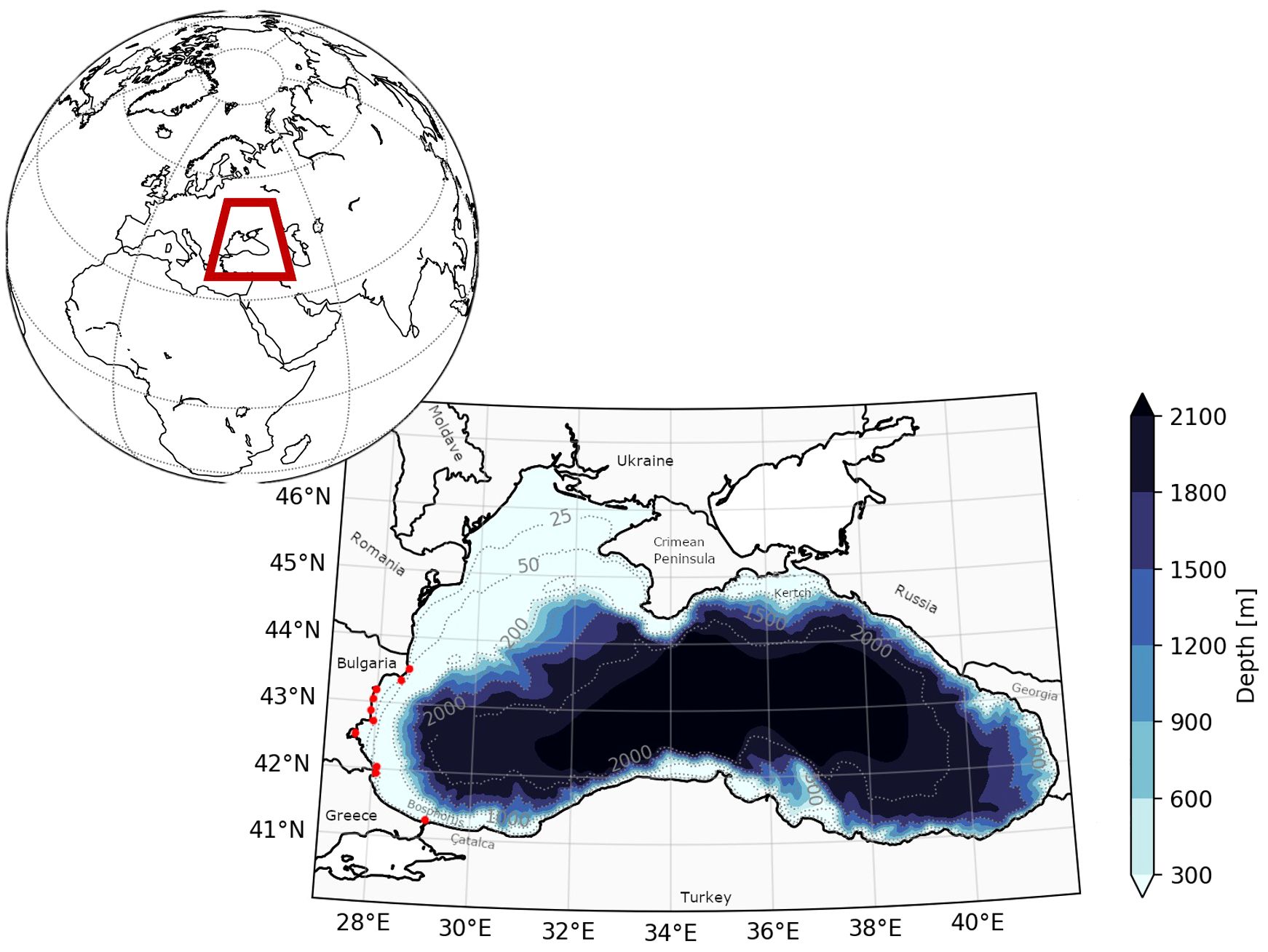
Figure 2 The Black Sea coastline and bathymetry. The moorings used for results validation are denoted by red dots.

2.4 Computation of variable statistics

In this study, we examined the SWH and MWD variables. We preferred to exclude the wave period from the study because we had limited data for validation, and from the initial investigations, its variability appeared to be very low compared to the variability of SWH.

Four metrics have been computed on a daily basis: 5th percentile, mean, 95th percentile, and maximum. While SWH needs no details, MWD requires some specification.

Due to the periodical nature of the directions, it is not possible to proceed with statistics computation as for other wave fields. Below, we provide the convention adopted for the definition of the direction associated with each of the four metrics. Please consider that we adopted circular statistics for the direction variable, according to Jammalamadaka and Sengupta (2001).

The direction of the SWH 5th percentile has been computed as the mean of the direction components of waves with SWH ≤ 5th percentile threshold.

The direction of the mean SWH has been computed as the mean of the direction components over the time frame of the study.

The direction of the SWH 95th percentile has been computed as the mean of the direction components of 94th percentile ≥ SWH ≤ 96th percentile.

Lastly, the direction of the SWH maximum has been computed as the mean of the direction components of waves with SWH ≥ 98th percentile threshold.

2.5 Trend assessment

The presence of a trend affecting the SWH during the investigated time frame has been assessed using a Mann–Kendall test (Mann, 1945; Kendall, 1970; Gilbert, 1987) (hereafter MK). The MK test is a non-parametric method employed to assess the presence or absence of a monotonic upward or downward trend of the variable of interest across time. In this study, a significance level of α = 0.05 was adopted, leading to rejection of the null hypothesis (indicating no trend in the dataset) for p-value< α.

The MK test has been applied to each of the statistical descriptors mentioned in the previous paragraph (mean, max, and 5th and 95th percentiles), both at the basin scale, for the assessment of a general trend all over the Black Sea, and to each point of the discretized domain, for the investigation of the spatial distribution of trends.

Figure 3

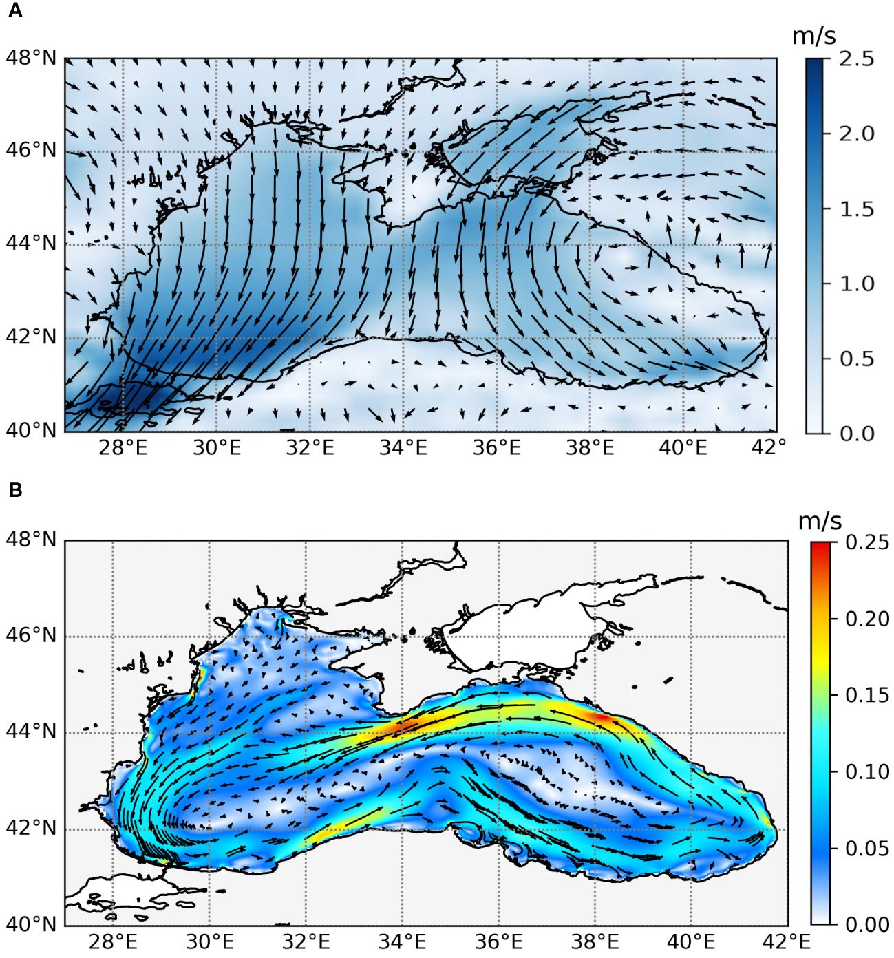
Figure 3 (A) Averaged [1988–2021] wind speed and direction (arrows) from ECMWF-ERA5. (B) Averaged [1988–2021] sea surface velocity and directions (arrows) from BLKMY Copernicus Marine Service.

3 Results and discussion

3.1 Model validation

The skill assessment has been based mainly on satellite data (Figure 4A), because this dataset has a full covering of the domain and many valid observations (~120,000). According to the data availability (e.g., few in situ buoys) and coverage, satellite validation resulted in the optimal solution for validating our regional model. The comprehensive coverage provided by the satellite offers an overall insight into the model quality. In contrast, wave in situ observation, while providing high-quality measurement, is often limited to coastal areas, where the climate model may lack adequate resolution, and it is generally rare.

Figure 4

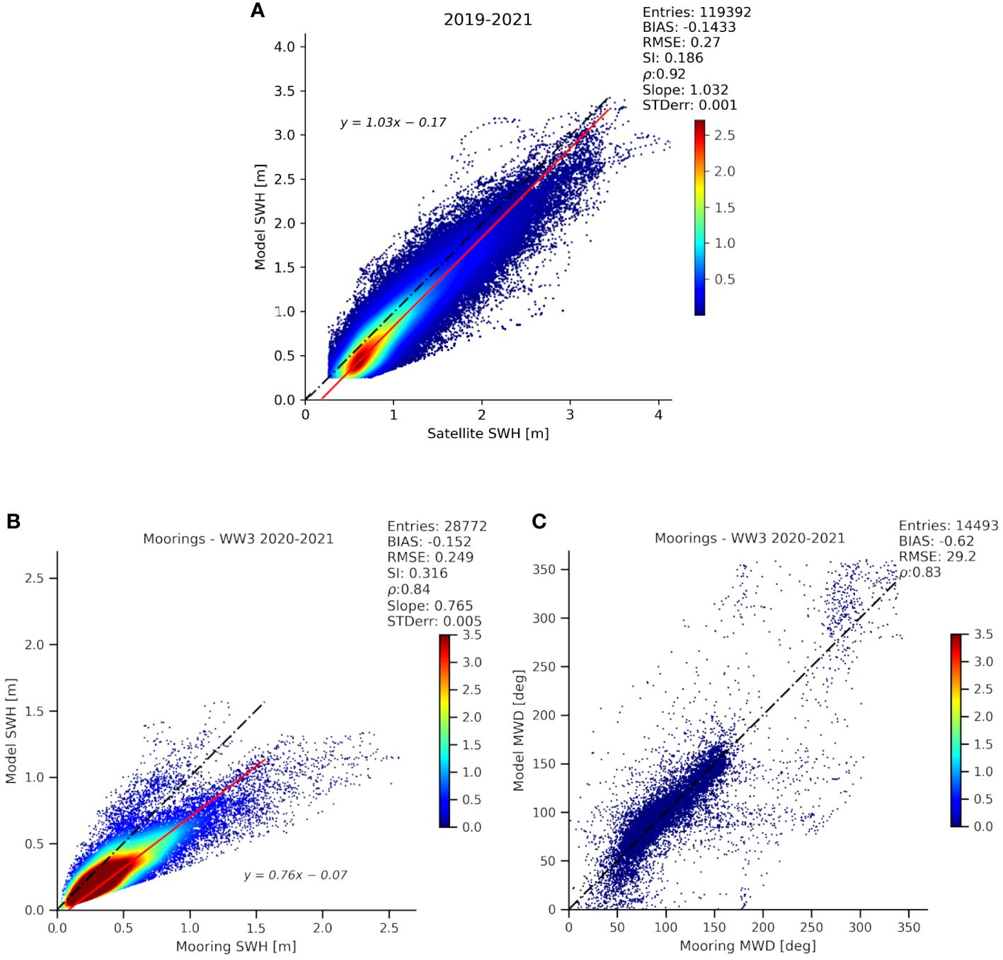
Figure 4 Scatter plot of SWH for WAV1 experiment compared to satellite observations (A) (data availability from July 2019 to December 2021). Scatter plots of SWH (B) and MWD (C) for WAV1 experiment compared to mooring observations (data availability from January 2020 to December 2021). Black dashed line represents the best fit, and red solid line (in A, B) indicates the slope of the least squared fit.

The REF configuration produced satisfactory skills: an SWH RMSE lower than 30 cm, a bias of −17 cm, and a correlation of 0.91. The statistical assessment of the model quality closely aligns with the WW3 implementation published by Soran et al. (2022). In their study, the authors are deeply dedicated in optimizing WW3 configuration forced by ERA5 for the BS region, obtaining slightly better results than ours (e.g., correlation 0.92 vs. 0.91, RMSE 0.27 vs. 0.29). However, the model configuration of Soran et al. (2022) is based on a finite element method, while in this work, we used a finite-difference method; thus, the setup cannot be considered the same. Nevertheless, our study is primarily focused on climate description, and the obtained results can be deemed satisfactory for the intended purposes.

From an overall perspective, the WAV1 experiment was revealed to be the best implementation; for that reason, it represents the simulation chosen for the climate description for the Black Sea region. The scatter plot distribution showed that the simulation fitted the best-fit line almost exactly, with a regression slope ~1.03, and the most common SWH values spanning between 0.3 and 1 m.

Figures 4B, C show the model validation with respect to the moorings available for the basin. As expected, mooring observations have a high frequency signal because of the sensitivity of the instrument, the very precise measurement in space, and the reduced number of available observations (~28,000). Additionally, the available moorings are located very close to the coast, and reduced accuracy arises due to the intricate coastal dynamics that may not be adequately represented by the model, particularly when considering its resolution at 3 km. It is noteworthy to mention that for MWD, the statistical computations were conducted with consideration for the periodic nature of the variable.

In Table 2, we summarized the main statistics for the two numerical experiments. The inclusion of the impact of currents on waves induced a slight skills improvement in the SWH, reducing both bias and RMSE by about ~20% and ~6% respectively. The addition of other hydrodynamic fields, such as sea level and air–sea temperature difference as wave forcing, induced no changes or slight performance degradation of SWH with respect to WAV1. From our perspective, sea level did not affect the SWH because its effect is evident only in shallow waters, while the BS is largely a deep basin, while the low resolution of ERA5 inputs negatively influenced the model results when air temperature difference is used.

Table 2

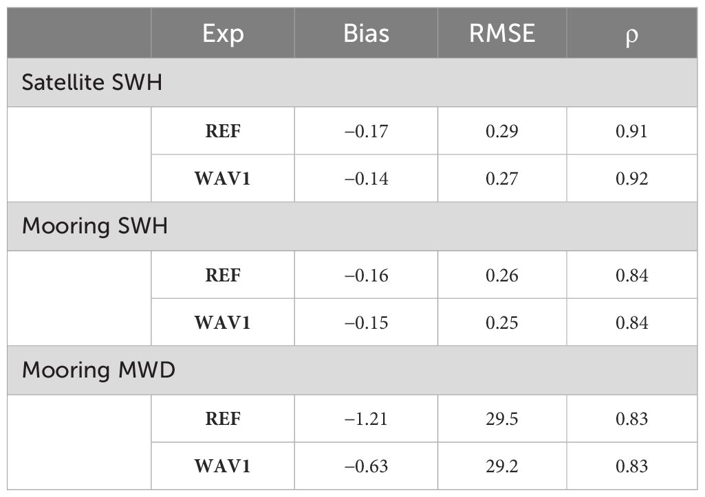
Table 2 Skills (BIAS, RMSE, and correlation) of numerical experiments compared to satellite (SWH) and mooring (SWH and MWD) observations.

The assessment of the SWH wave model skills with respect to moorings (Table 2) confirmed the improvement induced by currents when included in the wave simulation (RMSE −4%, bias −6%). Even regarding MWD, current forcing induced a quality improvement, mainly related to the bias reduction (−50%).

Table 3

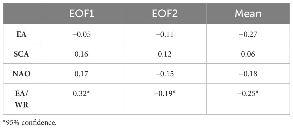
Table 3 Correlation between significant wave height average field and first two EOFs and main teleconnection indices for the Black Sea region.

The WAV1 configuration improved model accuracy with respect to the REF (only wind driven). Consequently, the simulation for the assessment of the BS wave climate has been carried out using the WAV1 setup. Under this climatological numerical setup, the inclusion of other hydrodynamic forcings (e.g., air–sea temperature difference and sea level) does not reduce or even affect the wave model skills.

Recently, Rybalko and Myslenkov (2022) investigated the role of currents in affecting the BS wave field. According to the authors, currents have a minimal impact on SWH, and the validation results indicated a marginal reduction of the model performance. These results are in agreement with what has been previously described in earlier works (Clementi et al., 2017; Causio et al., 2021). According to that, our recent findings seem to show a different behavior. The explanation of the differences could be attributed to the resolution of forcing fields adopted in the studies. Clementi et al. (2017) and Causio et al. (2021) used high-resolution (1/8°) atmospheric fields, and in both studies, the hydrodynamic field that improved the wave simulation was the air–sea temperature difference. Despite ERA5 atmospheric reanalysis having the highest available resolution (1/4°) for such products, it remains too coarse to significantly impact these processes. Similarly, Rybalko and Myslenkov (2022) employed a current field at 1/4°, potentially influencing the results in a comparable manner.

The inclusion of currents in the wave simulations mainly influenced the coastal areas (Figure 5), where, in most of the cases, mesoscale activity induced an SWH increase. In contrast, a negligible reduction is observed along the Rim current and the eastern basin, with a a peak approximately −3% close to the Georgia coasts. This peculiar pattern is attributed to the combined effect of wave and current intensity and their orientation.

Figure 5

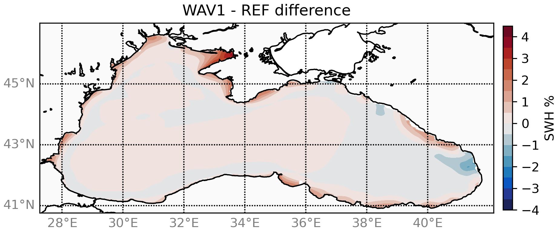
Figure 5 Significant wave height (1988–2021 average) difference between WAV1 and REF simulations, expressed in percentage.

Our findings validate Rybalko and Myslenkov’s (Rybalko and Myslenkov, 2022) assertion that the a priori application of current forcing in a wave model may not be an optimal solution. They further suggest that while using currents may be effective in certain scenarios, it may not be as beneficial in others. Therefore, it is advisable to conduct a thorough quality assessment of the wave model before incorporating currents. As such, the inclusion of currents should be evaluated on a case-by-case basis.

3.2 The Black Sea wave climate from 1988 to 2021

3.2.1 Intra-annual variability

This section describes the intra-annual variability of the wave field for the BS. Figure 6A shows how the monthly SWH varies over the yearly cycle. The SWH is highest in the winter months (Dec–Feb) with a mean of about 1 m throughout this period. In spring, the mean SWH sees a sharp decline to a minimum of approximately 50 cm in May and June. In the second half of the year, the mean SWH gradually increases again. The range of variation is relatively stable, with the years contained within a window of 20 cm (summer) to 40 cm (winter).

Figure 6

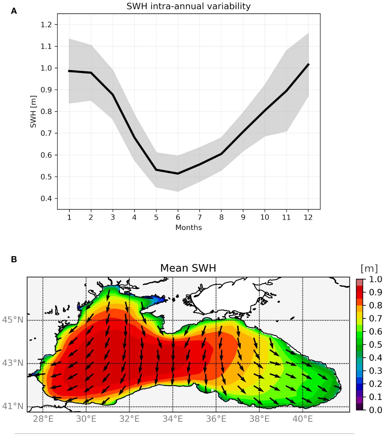
Figure 6 (A) Basin-averaged annual significant wave height variability, computed over the years 1988–2021. The solid black line highlights the mean; the associated standard deviation is in shaded gray. (B) The plot shows the geographic distribution of the mean wave height field and its related direction.

The geographic distribution of the mean SWH and wave direction is shown in Figure 6B. It shows a clear separation between the Western (Wb) and Eastern (Eb) sub-basins. The Wb is characterized by N-NE oriented waves with mean SWH values reaching close to 1 m in the majority of the Wb. This wave pattern perfectly matches wind circulation, with northerly winds prevailing in the west and north of the sea (Özsoy et al., 1998; Schrum et al., 2001; Efimov and Anisimov, 2011).

The Eb, on the other hand, shows N-NW oriented waves and a decrease in mean SWH to a minimum of 0.4 m in the easternmost part. The calmest areas of the sea are its southeastern and northwestern parts. The former is not highly affected by the impact of cyclones, whereas the latter is the widest shelf area in the BS, where wave growth is limited by the action of bottom friction (Arkhipkin et al., 2014).

The spatial variations of the mean SWH have been further investigated on a seasonal basis.

In the study, we adopted the conventional methodology in ocean season definition:

● Winter: December, January, February (DJF);

● Spring: March, April, May (MAM);

● Summer: June, July, August (JJA); and

● Autumn: September, October, November (SON).

Figure 7, subplots 1, shows the SWH for each season in terms of the mean, maximum, and 5th and 95th percentiles, while the arrows indicate the direction corresponding to each statistic.

Figure 7

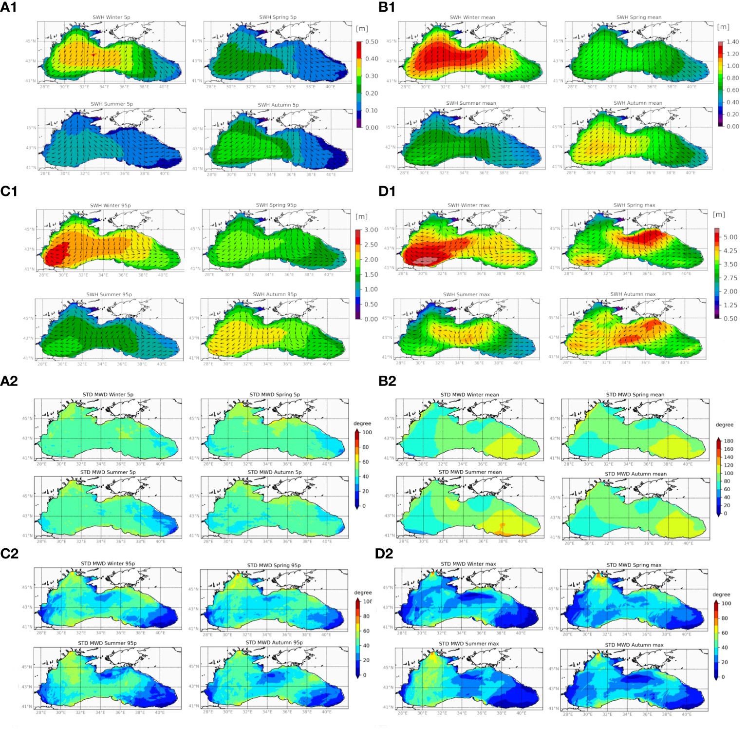
Figure 7 Uppermost four (A1–D1) shows statistical descriptors of seasonal significant wave height and wave direction. (A1) shows the 5th percentile; (B1) shows the mean; (C1) shows the 95th percentile; and (D1) shows the maximum. In each panel, the top left sub-plot refers to winter, the top right refers to spring, the bottom left refers to summer, and the bottom right refers to autumn. The lowermost four (A2–D2) indicate the seasonal standard deviation of MWD. (A2) shows the 5th percentile; (B2) shows the mean; (C2) shows the 95th percentile; and (D2) shows the maximum.

The mean and 5th/95th percentiles clearly show the difference between the rougher Wb and calmer Eb. The mean direction follows almost the same pattern throughout all the seasons, similar to the annual average.

The maximum SWH shows an interesting distribution. In winter, it is in line with the other distributions, with the highest values located between the Bosphorus and the Turkish Çatalca peninsula. In spring, however, the maximum SWH occurs in the Crimean–Kerch–Russian area in the calmer Eb. In summer and autumn, the maximum SWH occurs more towards the central Black Sea.

In addition, an increase in the frequency of western, southwestern, and southern waves is evident during spring and summer, arguably due to the influence of the Azores High pressure system (Bondar, 2014).

The main direction of the wave field is in agreement with the literature (Arkhipkin et al., 2014; Divinsky and Kosyan, 2017), showing waves are mainly NE-oriented except for the eastern part of the eastern basin, in which waves are NW-oriented. This pattern is evident for lower waves, 5th percentiles, and the mean wave height, while higher waves (95th percentile and maximum) showed a different pattern: SE waves along the west coast all through the year, and W-SW waves along the east coast.

In Figure 7, subplots 2, we illustrated the wave direction variability associated with the directions described in Figure 7, subplots 1. The most uncertain wave direction field is represented by the mean, which has an eastward increase of STD from ~80° to ~120° in all seasons.

All the other statistics manifested a lower variability in direction, in general below 60°. The lower waves (5th percentile) revealed a larger variability with respect to the higher waves (95th percentile and maximum), with a westward increase that spans from ~20° of the Eb to ~50° of the Wb. The higher waves exhibited the largest variability in the northwest of the basin and in the Kerch area, exceeding 70° in some cases. In contrast, the central part of the basin (south of the Crimean Peninsula) and the Wb, which showed the most stable directions, are affected by south-westerly and north-easterly winds, respectively.

The seasonality of the wave field can be further summarized by the seasonal variation index (SV) (Reguero et al., 2013). We excluded MWD from the analysis because the SW index is not suitable for the variable. The index quantifies the range of variation in mean seasonal values in relation to the annual mean, as follows:

$$SV=\frac{\overline{V_{Smax}}-\overline{V_{Smin}}}{{\overline{V}}_{mean}}$$

where V_Smax represents the maximum value of seasonal means, V_Smin is the minimum, and V_mean represents the total mean of the variable under consideration. Figure 8 shows the index expressed as a percentage. The index allows a sharp identification of the seasonality variation over the basin, showing a general reduction of the SV index from north (~60%variation) to south of the basins (~ 30%variation). The northeast coasts, including the Eastern Crimean Peninsula and the Russian BS coast, exhibit the highest variation, exceeding 80%. This notable peak in SWH variability could be attributed to the extreme wind variability of the area that has been described in a previous study (Akpınar et al., 2016). Notably, this area showed the occurrence of high maximum SWH values during the spring and autumn seasons, but also the very low 5th percentile (Figure 7, subplots 1).

Figure 8

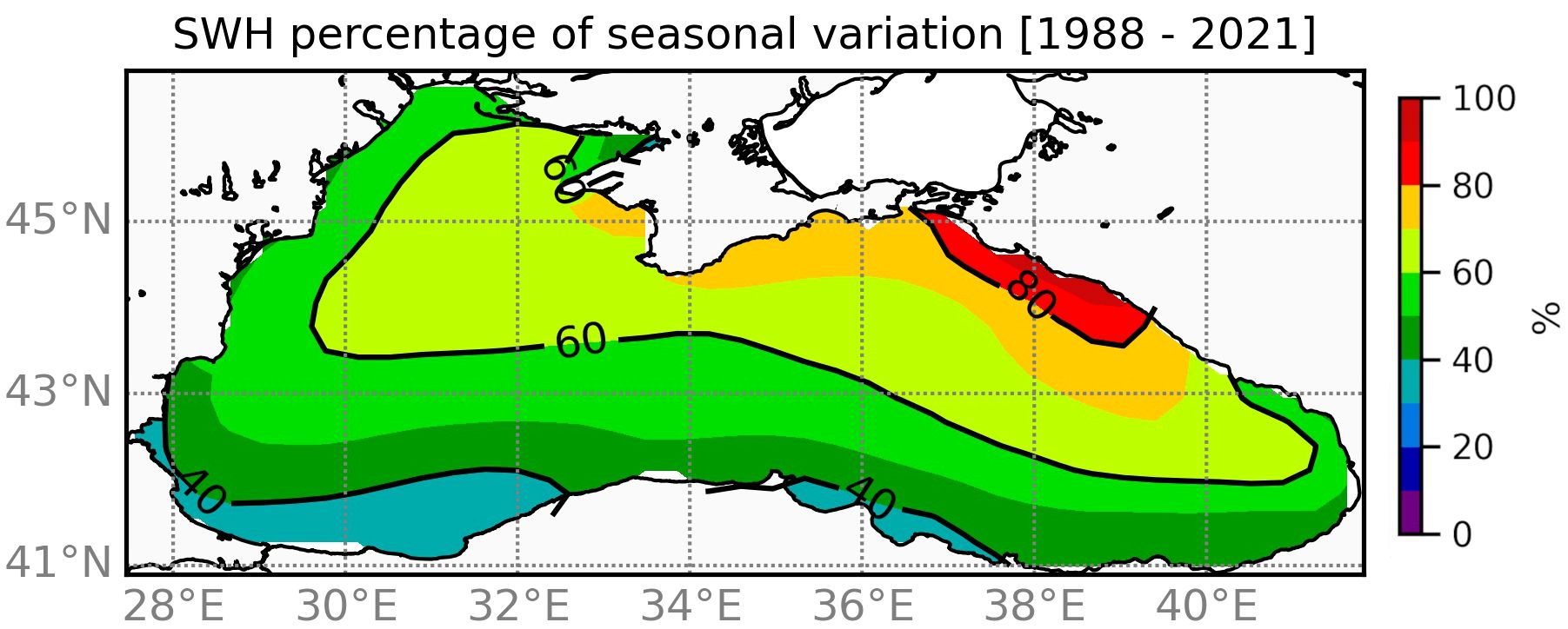
Figure 8 Seasonal variation index (expressed in percentage) for significant wave height.

3.2.2 Inter-annual variability

In the following section, the inter-annual variability of SWH has been analyzed in terms of the principal mode of variability, both cumulative and at basin scale, and also as geographic distribution of seasonal statistics.

The wave field variability of SWH and wave direction have been computed by PCA. This statistical technique (Zwiers and von Storch, 2004) is extensively applied in climatological analyses. It enables the identification of meaningful components amidst the extensive amount of data, distinguishing them from “noise”, which may be irrelevant in the process of description and understanding the real system (Lionello and Sanna, 2005). PCA is founded on an eigenproblem derived from maximizing the quadratic propriety of the variance. The data transformed through this process delineate the Empirical Orthogonal Functions (EOFs), which represent orthogonal spatial patterns that identify the preferred modes of variability within the system. Principal components (hereinafter, PC) capture the variability of the field and represent the temporal coefficients obtained by projecting the fields onto the EOFs.

In this investigation, the PCA has been applied to SWH, generating a vector with magnitude SWH and direction representing the MWD. Most of the SWH variability is described by the first two EOFs, accounting for 67% and 15% of the total variance (Figure 9C).

Figure 9

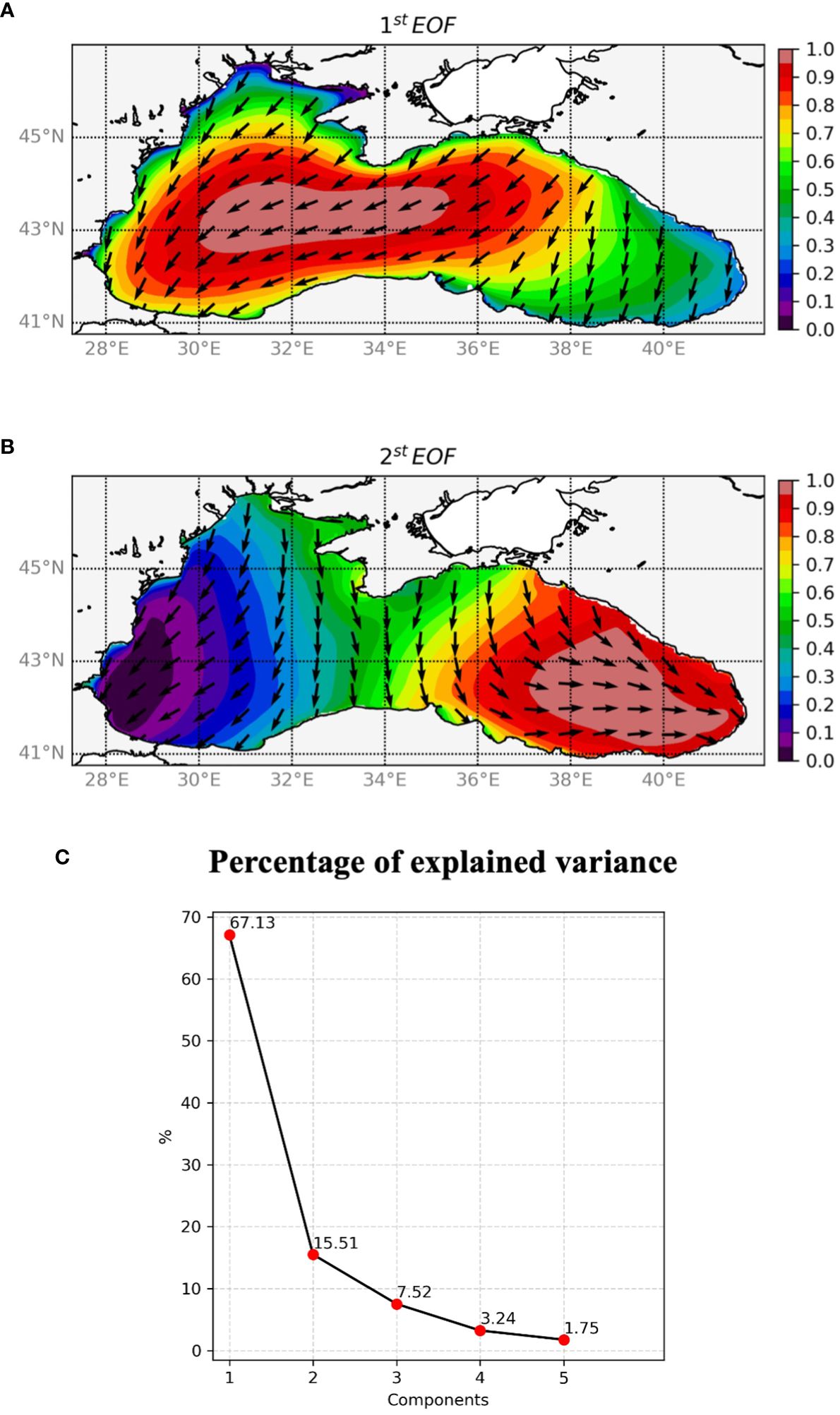
Figure 9 Spatial distribution of 1st (A) and 2nd (B) EOFs via PCA. All patterns are normalized with their maximum value. Arrows show wave direction. (C) Percentage of explained variance for the first five Empirical Orthogonal Functions. The values represent the proportion to which the EOFs account for the deviation of the SWH field during a year.

The firstEOF (Figure 9A) represents northeastern waves in the Wb and central BlackSea, as a result of the prevailing northerly winds. Instead, the second EOF (Figure 9B) represents the south-southeastern propagating waves in the Eb. The PCA therefore confirms, as far as the wave climate is concerned, the division of the Black Sea into Eastern and Western sub-basins, as we proposed before.

The characterization of the first two EOFs was established through an examination of the composites of SWH (Figure 10, subplots 1) and mean sea level pressure (MSLP) (Figure 10, subplots 2). In generating each composite, we differentiated between upper and lower phases by considering the average fields of the SWH and MSLP when the associated EOF of the SWH field was in the uppermost/lowermost 10%.

Figure 10

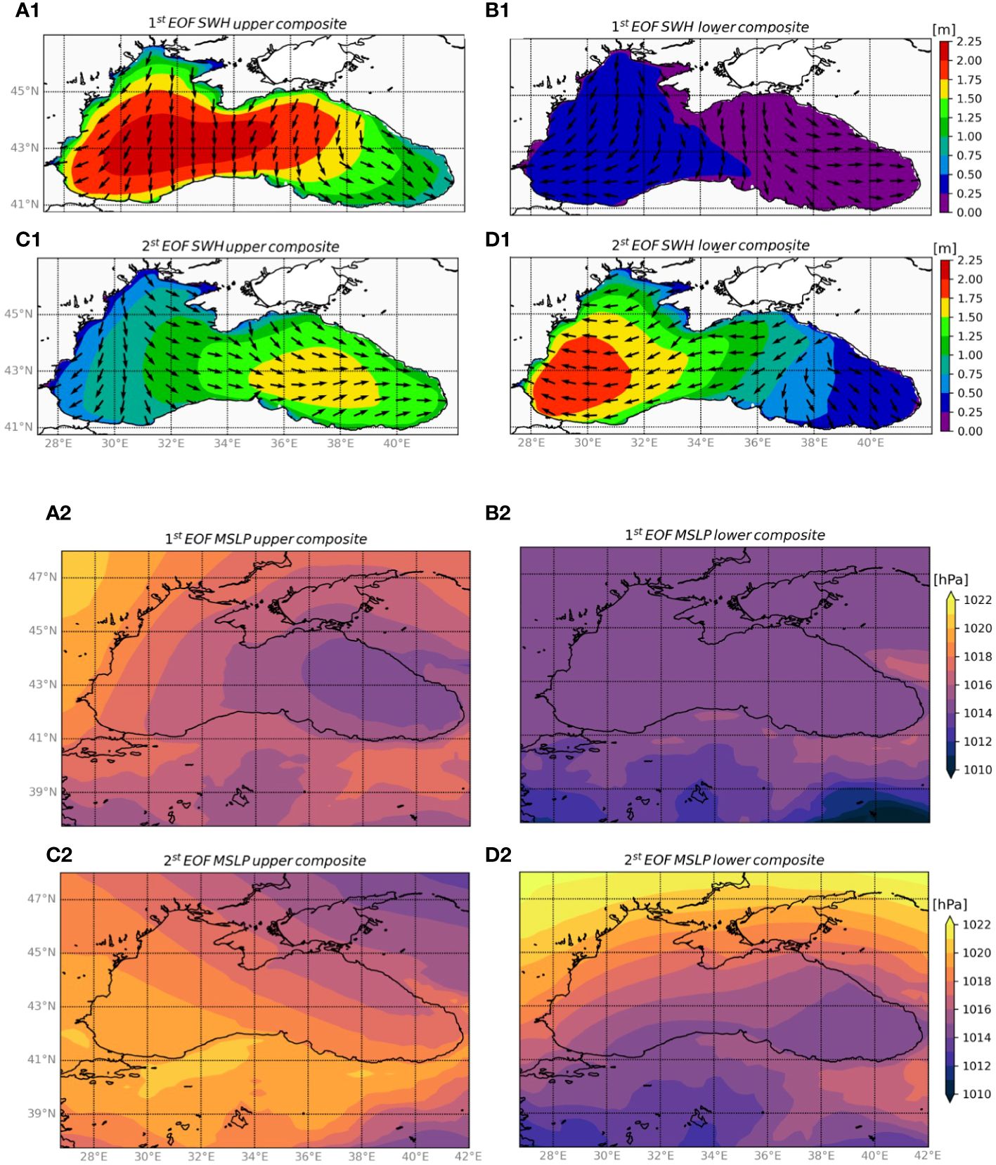
Figure 10 The uppermost four subplots, labeled with 1, show upper (A1–C1) and lower (B1–D1) composites of SWH and corresponding direction (arrows) computed using the 1st EOF (A1–B1) and the 2nd EOF (C1–D1). The lowermost four subplots, labeled with 2, show the corresponding composites for mean sea level pressure (MSLP).

The main mode for the wave climate in the BS is described by Figure 10A1. This wave field is generated by low pressure located in the Eb along Russian coasts (Figure 10A2) and high pressure in central-western Europe, defining rougher waves in the Wb, mainly N-NE oriented, which exceeded 2 m in height. The lower composite of the first EOF is represented by very smooth wave conditions (Figure 10B1) and low pressure all over the BS domain (Figure 10B2).

The second mode of the BS wave field is shown in Figure 10C1 with NW-W waves exceeding 1.5 m in height in the Eb. This condition is generated by high pressure in Turkey and low pressure in the northeast of the Azov Sea (Figure 10C2). The lower composite of EOF2 shows E-oriented waves, except for the eastern part of the Eb. This wave field provided high waves (exceeding 1.75 m) in the southwest region of the BS, and is defined by low pressure in southern Turkey and high pressure above 47°N.

Therefore, both time and space coefficients have been projected onto cumulative yearly EOFs to highlight the variability of the principal components between years. Figure 11 denoted that, in the last three decades, the first two EOFs had opposite trends, with the weakening of EOF1 and the strengthening of EOF2, even if to a lesser extent: −9% for EOF1 and +4.5% for EOF2. This tendency can be interpreted as the reduction of N-NE waves, mainly driven by winds developed in the MSLP dipole shown in Figure 10A2, in favor of the frequency intensification of W-oriented waves for Eb (Figure 10C2).

Figure 11

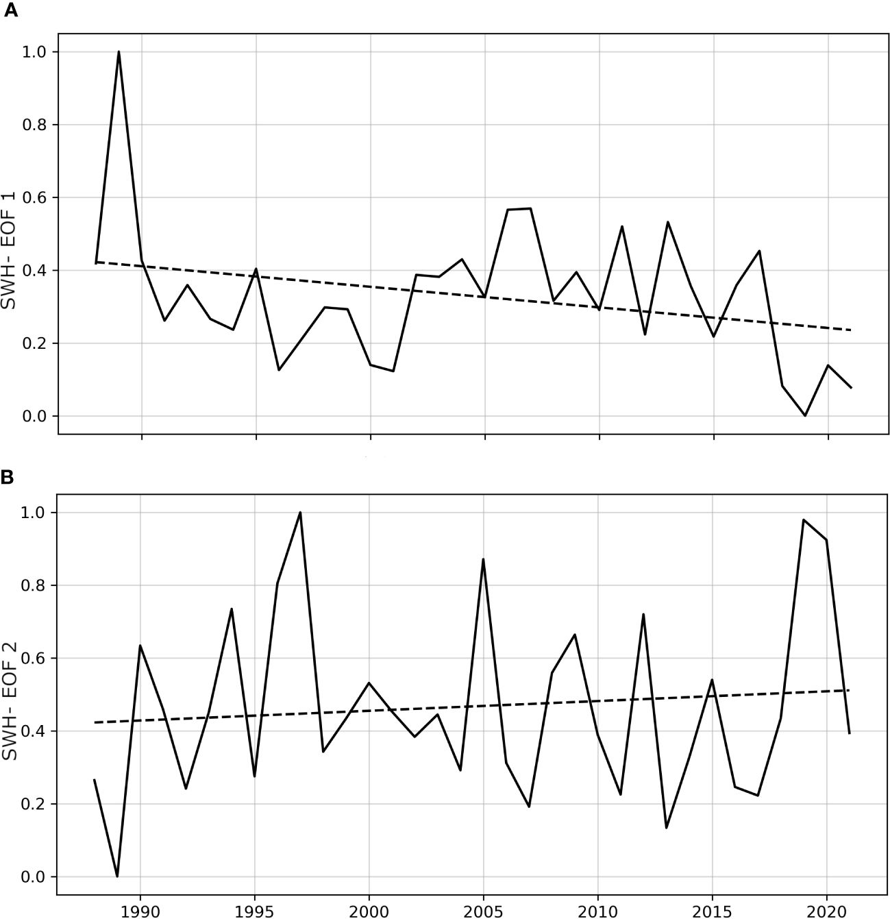
Figure 11 First (A) and second (B) normalised timeseries of SWH EOF, scaled by the square root of their eigenvalue, are shown as solid lines, while the dashed lines indicate the statistically significant trends (p-value<0.05).

From an MSLP perspective, the changes could be intended as the shifting of higher pressure towards Turkey and the displacement of lower pressure toward the eastern Azov Sea.

The trend analysis through the MK test over the time frame 1988–2021 did not reveal any significant change in SWH climate at basin scale, for all the statistics (5th–95th percentiles, mean, and maximum). There was no statistically significant trend, even when the test was applied at a seasonal scale.

Furthermore, the trend assessment has also been applied in the spatial domain, as depicted in Figure 12. To enhance the plotting clarity, results of the MK test for SWH are presented in a reduced resolution of approximately 1/3°. Trend values with significance lower than 95% are rejected and masked in the figure.

Figure 12

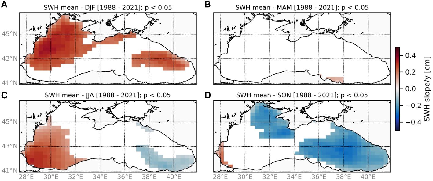
Figure 12 Spatial distribution of statistically significant (p< 0.05) trends [cm/year] for mean significant wave height for winter (A), spring (B), summer (C), and autumn (D).

The seasonal trend investigation (Figure 12) provided a similar spatial pattern between all the statistical descriptors. Two seasons showed a wider spatial covering affected by significant trends for SWH. In winter, a near-majority of the basin (mostly the Wb) is affected by a positive trend, while during autumn, almost all the basin (mostly the Eb) shows a negative trend. The MK test highlighted the absence of trends in spring and a well-defined distinction between the Wb (positive trend) and Eb (negative trend) during summer. The strength of the trend increased as the waves increase: on the average field, the SWH trends varied within a range of ± 0.25 cm/year, while for the highest waves’ statistics (95th percentile and max), the range was ± 0.5 cm/year.

Our comprehensive analysis of the wave inter-annual variability for the BS reveals rougher sea conditions during winter, in contrast with calmer sea conditions during autumn. We hypothesized that the negative trend in autumn may be driven by the increased frequency of lower EOF1. On the other hand, the positive trend during winter in the Eb appears to be dependent on the changes observed in upper EOF2 and MSLP composites, as detailed previously. Concerning the positive trend of the Wb waves, we could not establish a direct association with any of the investigated composites, leading us to conclude that the trend is likely to be related to less recurrent composites.

3.2.3 Teleconnections

The last section of the study assessed the relationship between the most important atmospheric teleconnections (TLC) and SWH for the BS domain: East Atlantic Pattern (EA), Scandinavian Pattern (SCA), North Atlantic Oscillation (NAO), and East Atlantic/West Russia Pattern (EA/WR). The indices time series have been provided by https://www.cpc.ncep.noaa.gov/data/teledoc/telecontents.shtml.

One of the most important teleconnection patterns across seasons is the NAO, as identified by Barnston and Livezey (1987). The NAO manifests as a north–south dipole of anomalies, featuring one center situated over Greenland and the other center with an opposite sign, extending across the central latitudes of the North Atlantic. The NAO is characterized by two phases.

The EA pattern emerges as the second significant mode of low-frequency variability over the North Atlantic. It comprises a north–south dipole of anomaly centers spanning from east to west across the North Atlantic. However, the EA pattern is distinguished from the NAO by the lower-latitude center location and its association with the subtropical ridge.

The EA/WR pattern stands out as a key teleconnection pattern influencing Eurasia, characterized by four primary anomaly centers.

The SCA comprises weak centers of opposite signs over western Europe and eastern Russia/western Mongolia (Barnston and Livezey, 1987), governing a primary circulation center over Scandinavia.

3.2.4 Correlation with teleconnections

The correlation between TLC patterns and SWH fields has been evaluated on a monthly basis, both on the averaged wave field and EOFs. The analysis was limited to the winter season, characterized by active cyclogenesis above the Mediterranean and the Black Sea (Mikhailova and Yurovsky, 2016). During this period, a high-pressure system dominates central Europe, positioned between two pressure centers, over western Russia and the mid-Atlantic.

The investigation revealed that only the EA/WR pattern, for both EOFs and the mean field, has a statistically significant TLC–SWH correlation (p-value<0.05). In detail, from the correlation matrix (Table 3), we observed that the EA/WR pattern showed the largest influence on the wave variability, mainly on EOF1 (0.32), and the pattern is negatively correlated with EOF2 to a lesser extent (−0.19). Considering the mean wave condition of the last three decades at basin scale, the correlation was negative (−0.25). This finding offers new perspectives on the correlation between BS wave and TC indices. It is noteworthy that in the earlier research of Saprykina et al. (2019), the annual mean waves were found to be more affected by the NAO. However, it is important to consider that the two studies investigated different time frames.

An investigation of the spatial distribution of the correlation has shown that the link between TLC patterns and mean SWH is not uniform across the BS basin (Figure 13). Considering the different characteristics of the sub-basins, this is to be expected, as already found and described by Lionello and Galati (2008) for the Mediterranean Sea.

Figure 13

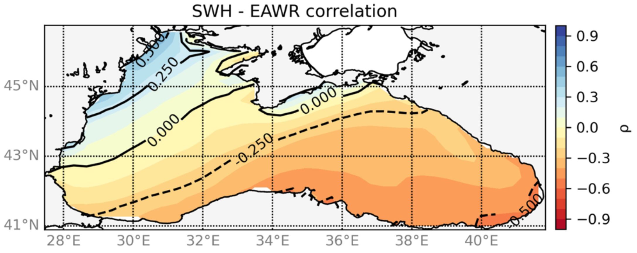
Figure 13 Correlation map of the EA/WR index and SWH over the 1988–2021 index for the winter season.

Spatially, most of the domain presented a negative TLC-SWH correlation with an intensification towards the southeast, exceeding −0.5 along the east coasts.

In contrast, the EA/WR pattern has a strong positive link with SWH along the western coasts of Ukraine. This spatial correlation pattern is in agreement with findings from Saprykina et al. (2019). In addition, this investigation revealed no or low correlation for the central part of the Wb along the continental slope.

The correlation analysis indicated the BS wave climate’s clear dependency on the EA/WR pattern, for both its variability (EOFs) and mean. However, the stronger correlation with EOF1 reveals that when the EA/WR pattern is stronger, the seasonal cycle is more intense. The spatial correlation confirmed the distinction between the Wb and Eb wave field that we observed in the previous analyses. During its positive phase, the EA/WR pattern consists of four centers: two positive height anomalies located over north-central Europe and northern China, and two negative height anomalies located over the central North Atlantic and north of the Caspian Sea.

The correlation map accurately matches the dipole pattern located in Europe and Russia, determining a strong positive correlation in the northwestern basin and a strong negative correlation with the southeastern basin.

4 Conclusions

This study presents the Black Sea wave climate for the period 1988–2021 simulated by using a dedicated implementation of the WAVEWATCH III wave model, forced by wind from the ECMWF ERA5 reanalysis. The investigation is based on an unprecedent horizontal resolution for a BS wave climate study at the basin scale. In addition, the study represented the opportunity to investigate the role of the wave–current interaction in a climate study.

The model calibration required a specific tuning of the input source term in order to mitigate the SWH underestimation, particularly for high waves, when utilizing ERA5 winds.

Interestingly, the comparison model observations revealed that the inclusion of current forcing slightly enhanced the model quality, while no significant improvements are evident when sea level and air–sea temperature difference is applied. This result, in comparison with previous studies (Clementi et al., 2017; Causio et al., 2021; Rybalko and Myslenkov, 2022), reveals how important is the assessment of hydrodynamic forcing for any specific modeling implementation and region.

An extensive statistics description of the Black Sea intra-annual wave cycle has been carried out for SWH and related direction. The association of the wave direction to a specific statistic of the SWH has been proposed as a methodology and is detailed in Section 2.4.

Geographically, the basin can be divided into an Eastern (Eb) and Western sub-basin (Wb). The Wb typically experiences higher SWH and predominantly N-NE oriented waves. The Eb exhibits N-NW oriented waves with decreasing SWH towards the east.

While no overall trends were identified when considering the investigated time range, the study revealed distinctive patterns influenced by seasonal dynamics: SWH decreases in late summer and autumn in the Eb, leading to a prolongation of summer conditions in that area. In winter, when SWH is typically the largest, it increases further in both the Eb and Wb. In summer, there is also an increase in SWH in the southwestern Black Sea. The spring season appears to be unaffected by these trends.

The Black Sea wave climate is governed by two main modes of variability. The first mode is characterized by waves generated by low pressure along the Russian coasts and high pressure in central-western Europe, resulting in rougher waves in the western basin predominantly oriented N-NE. The second mode features NW-W waves in the eastern basin influenced by high pressure in Turkey and low pressure in the northeast of the Azov Sea. Over the last three decades, there has been a weakening of N-NE waves and an increase in W-oriented waves, likely due to changes in atmospheric pressure distribution.

The study of atmospheric teleconnection patterns highlighted the significant influence of the East Atlantic/West Russia Pattern (EA/WR) on SWH, emphasizing distinctions between the eastern and western basin wave fields.

Spatially, most of the domain exhibited a negative TLC-SWH correlation, intensifying towards the southeast. However, the EA/WR pattern showed a strong positive correlation with SWH along the western coasts of Ukraine. The correlation analysis confirmed the BS wave climate’s strong dependency on the EA/WR pattern, impacting both variability and mean conditions.

Overall, the study contributes to a better understanding of the spatiotemporal variability of wave fields in the region, which is significant information for various applications such as coastal engineering, marine operations, and climate studies.

Data availability statement

The raw data supporting the conclusions of this article will be made available by the authors, without undue reservation.

Author contributions

SC: Writing – review & editing, Writing – original draft, Visualization, Validation, Software, Methodology, Investigation, Formal Analysis, Data curation, Conceptualization. IF: Writing – review & editing, Methodology, Conceptualization. EJ: Writing – review & editing, Supervision, Investigation, Conceptualization. LM: Writing – review & editing, Supervision, Methodology, Investigation, Formal Analysis. SAC: Writing – review & editing, Supervision, Methodology, Investigation. GC: Writing – review & editing, Supervision, Resources. PL: Writing – review & editing, Methodology, Formal Analysis, Conceptualization.

Funding

The author(s) declare financial support was received for the research, authorship, and/or publication of this article. This research was funded by the Copernicus Marine Service for the Black Sea Monitoring and Forecasting Center (Contract n./ref.: 21002L04-COP-MFC-BS-5400).

Conflict of interest

The authors declare that the research was conducted in the absence of any commercial or financial relationships that could be construed as a potential conflict of interest.

Publisher’s note

All claims expressed in this article are solely those of the authors and do not necessarily represent those of their affiliated organizations, or those of the publisher, the editors and the reviewers. Any product that may be evaluated in this article, or claim that may be made by its manufacturer, is not guaranteed or endorsed by the publisher.

Supplementary material

The Supplementary Material for this article can be found online at: https://www.frontiersin.org/articles/10.3389/fmars.2024.1406855/full#supplementary-material

Abbreviations

BS, Black Sea; WW3, WAVEWATCH III; CMS, Copernicus Marine Service; ECMWF, European Centre for Medium-Range Weather Forecasts; BLKMY, Black Sea multi-year; NRT, Near real time; SWH, Significant wave height; MWD, Mean wave direction; EOF, Empirical orthogonal function; EA, East-Atlantic teleconnection pattern; SCA, Scandinavia teleconnection pattern; NAO, North Atlantic Oscillation teleconnection pattern; EA/WR, East Atlantic/West Russia teleconnection pattern; Wb, Black Sea Western basin; Eb, Black Sea Eastern basin; PC, Principal component; SV, Seasonal variation.

Footnotes

1. ^ Black Sea Physics Reanalysis (Copernicus Marine MyOcean). Available online at: https://data.marine.copernicus.eu/product/BLKSEA_MULTIYEAR_PHY_007_004/description (Accessed June 28, 2023).
2. ^ Global Ocean L 3 Significant Wave Height From Nrt Satellite Measurements. Available online at: https://data.marine.copernicus.eu/product/WAVE_GLO_PHY_SWH_L3_NRT_014_001/description (Accessed January 18, 2023).
3. ^ Black Sea- In-Situ Near Real Time Observations. Available online at: https://data.marine.copernicus.eu/product/INSITU_BLK_PHYBGCWAV_DISCRETE_MYNRT_013_034/description (Accessed January 18, 2023).

References

Acar E., Akpinar A., Kankal M., Amarouche K. (2023). Increasing trends in spectral peak energy and period in a semi-closed sea. Renewable Energy 205, 1092–1104. doi: 10.1016/j.renene.2023.02.007

CrossRef Full Text | Google Scholar

Akcay F., Bingölbali B., Akpınar A., Kankal M. (2022). Trend detection by innovative polygon trend analysis for winds and waves. Front. Mar. Sci. 9, 930911. doi: 10.3389/fmars.2022.930911

CrossRef Full Text | Google Scholar

Akpınar A., Bingölbali B., Van Vledder G. (2016). Wind and wave characteristics in the Black Sea based on the SWAN wave model forced with the CFSR winds. Ocean Eng. 126, 276–298. doi: 10.1016/j.oceaneng.2016.09.026

CrossRef Full Text | Google Scholar

Akpınar A., Ph G., van Vledder M., Kömürcü İ., Özger M. (2012). Evaluation of the numerical wave model (SWAN) for wave simulation in the Black Sea. Continent. Shelf Res. 50–51, 80–99. doi: 10.1016/j.csr.2012.09.012

CrossRef Full Text | Google Scholar

Alday M., Accensi M., Ardhuin F., Dodet G. (2021). A global wave parameter database for geophysical applications. Part 3: Improved forcing and spectral resolution. Ocean Model. 166, 101848. doi: 10.1016/j.ocemod.2021.101848

CrossRef Full Text | Google Scholar

Ardhuin F., Rogers E., Babanin A. V., Filipot J.-F., Magne R., Roland A., et al. (2010). Semiempirical dissipation source functions for ocean waves. Part I: Definition, calibration, and validation. J. Phys. Oceanogr. 40, 1917–1941. doi: 10.1175/2010JPO4324.1

CrossRef Full Text | Google Scholar

Ardhuin F., Bertotti L., Bidlot J. R., Cavaleri L., Filipetto V., Lefevre J. M., et al. (2007). Comparison of wind and wave measurements and models in the Western Mediterranean Sea. Ocean Engineering 34, 526–541.

Google Scholar

Arkhipkin V. S., Gippius F. N., Koltermann K. P., Surkova G. V. (2014). Wind waves in the Black Sea: results of a hindcast study. Natural Hazards Earth Sys. Sci. 14, 2883–2897. doi: 10.5194/nhess-14-2883-2014

CrossRef Full Text | Google Scholar

Barnston A. G., Livezey R. E. (1987). Classification, seasonality and persistence of low-frequency atmospheric circulation patterns. Monthly Weather Rev. 115, 1083–1126. doi: 10.1175/1520-0493(1987)115<1083:CSAPOL>2.0.CO;2

CrossRef Full Text | Google Scholar

Battjes J. A., Janssen J. P. F. M. (1978). Energy loss and set-up due to breaking of random waves. Coast. Eng. 1978, 569–587. doi: 10.1061/9780872621909

CrossRef Full Text | Google Scholar

Bondar C. (2014). Black sea oceanography. Geo-Eco-Marina 1.

Google Scholar

Booij N., Ris R. C., Holthuijsen L. H. (1999). A third-generation wave model for coastal regions, 1. Model description and validation. J. Geophys. Res. 104, 649–7,666. doi: 10.1029/98JC02622

CrossRef Full Text | Google Scholar

BS_INS_NRT. Black Sea- In-situ near real time observations. Available online at: https://data.marine.copernicus.eu/product/INSITU_BLK_PHYBGCWAV_DISCRETE_MYNRT_013_034/description (Accessed January 18, 2023).

Google Scholar

BS-PHY_REA. Black Sea Physics reanalysis (copernicus marine myOcean viewer). Available online at: https://data.marine.copernicus.eu/product/BLKSEA_MULTIYEAR_PHY_007_004/description (Accessed June 28, 2023).

Google Scholar

Çakmak R. E., Çalışır E., Lemos G., Akpınar A., Semedo A., Cardoso R. M., et al. (2023). Regional wave climate projections forced by EURO-CORDEX winds for the Black Sea and Sea of Azov towards the end of the 21st century. Int. J. Climatol. 43, 5927–5950. doi: 10.1002/joc.8181

CrossRef Full Text | Google Scholar

Çalışır E., Soran M. B., Akpınar A. (2023). Quality of the ERA5 and CFSR winds and their contribution to wave modelling performance in a semi-closed sea. J. Operation. Oceanogr. 16, 106–130. doi: 10.1080/1755876X.2021.1911126

CrossRef Full Text | Google Scholar

Causio S., Ciliberti S. A., Clementi E., Coppini G., Lionello P. (2021). A modelling approach for the assessment of wave-currents interaction in the black sea. J. Mar. Sci. Eng. 9, 893. doi: 10.3390/jmse9080893

CrossRef Full Text | Google Scholar

Cavaleri L., Bertotti L. (2006). The improvement of modelled wind and wave fields with increasing resolution. Ocean Eng. 33, 553–565. doi: 10.1016/j.oceaneng.2005.07.004

CrossRef Full Text | Google Scholar

Cavaleri L., Langodan S., Pezzutto P., Benetazzo A. (2024). The earliest stages of wind wave generation in the open sea. J. Phys. Oceanogr. 54, 755–766. doi: 10.1175/JPO-D-23-0217.1

CrossRef Full Text | Google Scholar

Ciliberti S. A., Grégoire M., Staneva J., Palazov A., Coppini G., Lecci R., et al. (2021). Monitoring and forecasting the ocean state and biogeochemical processes in the black sea: recent developments in the copernicus marine service. J. Mar. Sci. Eng. 9, 1146. doi: 10.3390/jmse9101146

CrossRef Full Text | Google Scholar

Ciliberti S. A., Jansen E., Coppini G., Peneva E., Azevedo D., Causio S., et al. (2022). The black sea physics analysis and forecasting system within the framework of the copernicus marine service. J. Mar. Sci. Eng. 10, 48. doi: 10.3390/jmse10010048

CrossRef Full Text | Google Scholar

Clementi E., Oddo P., Drudi M., Pinardi N., Korres G., Grandi A. (2017). Coupling hydrodynamic and wave models: first step and sensitivity experiments in the Mediterranean Sea. Ocean Dynam. 67, 1293–1312. doi: 10.1007/s10236-017-1087-7

CrossRef Full Text | Google Scholar

Divinsky B. V., Kos’ yan R. D. (2015). Observed wave climate trends in the offshore Black Sea from 1990 to 2014. Oceanology 55, 837–843. doi: 10.1134/S0001437015060041

CrossRef Full Text | Google Scholar

Divinsky B. V., Kosyan R. D. (2017). Spatiotemporal variability of the Black Sea wave climate in the last 37 years. Continent. Shelf Res. 136, 1–19. doi: 10.1016/j.csr.2017.01.008

CrossRef Full Text | Google Scholar

Divinsky B., Kosyan R. (2018). Parameters of wind seas and swell in the Black Sea based on numerical modeling. Oceanologia 60, 277–287. doi: 10.1016/j.oceano.2017.11.006

CrossRef Full Text | Google Scholar

Divinsky B. V., Kubryakov A. A., Kosyan R. D. (2020). Interannual variability of the wind-wave regime parameters in the Black Sea. Phys. Oceanogr. 27, 337–351. doi: 10.22449/1573-160X

CrossRef Full Text | Google Scholar

Dobricic S., Pinardi N. (2008). An oceanographic three-dimensional variational data assimilation scheme. Ocean Model. 22, 89–105. doi: 10.1016/j.ocemod.2008.01.004

CrossRef Full Text | Google Scholar

Dodet G., Piolle J.-F., Quilfen Y., Abdalla S., Accensi M., Ardhuin F., et al. (2020). The Sea State CCI dataset v1: towards a sea state climate data record based on satellite observations. Earth Sys. Sci. Data 12, 1929–1951. doi: 10.5194/essd-12-1929-2020

CrossRef Full Text | Google Scholar

Efimov V. V., Anisimov A. E. (2011). Climatic parameters of wind-field variability in the Black Sea region: Numerical reanalysis of regional atmospheric circulation. Izvestiya Atmos. Ocean. Phys. 47, 350–361. doi: 10.1134/S0001433811030030

CrossRef Full Text | Google Scholar

Gilbert R. O. (1987). Statistical Methods for Environmental Pollution Monitoring (Third avenue, New York: John Wiley & Sons).

Google Scholar

Günther H., Hasselmann S., Janssen P. A. (1992). The WAM Model Cycle 4 Edited by: Modellberatungsgruppe, Hamburg

Google Scholar

Gürses Ö. (2016). Dynamics of the Turkish Straits System: A Numerical Study with a finite element ocean model based on an unstructured grid approach (Ankara, Turkey: Middle East Technical University).

Google Scholar

Hasselmann K., Barnett T. P., Bouws E., Carlson H., Cartwright D. E., Enke K., et al. (1973). Measurements of wind-wave growth and swell decay during the Joint North Sea Wave Project (JONSWAP). Ergänzungsheft Zur Deutschen Hydrographischen Zeitschrift Reihe A, 12.

Google Scholar

Hasselmann D., Bösenberg J., Dunckel M., Richter K., Grünewald M., Carlson H. (1986). Measurements of wave-induced pressure over surface gravity waves, in Wave dynamics and radio probing of the ocean surface (Springer), 353–368. doi: 10.1007/978-1-4684-8980-4

CrossRef Full Text | Google Scholar

Hasselmann S., Hasselmann K., Allender J. H., Barnett T. P. (1985). Computations and parameterizations of the nonlinear energy transfer in a gravity-wave specturm. Part II: parameterizations of the nonlinear energy transfer for application in wave models. J. Phys. Oceanogr. 15, 1378–1391. doi: 10.1175/1520-0485(1985)015<1378:CAPOTN>2.0.CO;2

CrossRef Full Text | Google Scholar

Hersbach H., Bell B., Berrisford P., Hirahara S., Horányi A., Muñoz-Sabater J., et al. (2020). The ERA5 global reanalysis. Q. J. R. Meteorol. Soc. 146, 1999–2049. doi: 10.1002/qj.3803

CrossRef Full Text | Google Scholar

Holthuijsen L. H., Booij N., Bertotti L. (1996). The propagation of wind errors through ocean wave hindcasts. J. Offshore Mech. Arctic Eng. 3, 118. doi: 10.1115/1.2828832

CrossRef Full Text | Google Scholar

Holthuijsen L. H., Booij N., Ris R. C., Haagsma I. G., Kieftenburg A. T. M. M., Kriezi E. E. (2001). SWAN Cycle III Version 40.11 User Manual (Delft, The Netherlands: Delft University of Technology Press).

Google Scholar

Islek F., Yuksel Y., Sahin C. (2022). Evaluation of regional climate models and future wave characteristics in an enclosed sea: A case study of the Black Sea. Ocean Eng. 262, 112220. doi: 10.1016/j.oceaneng.2022.112220

CrossRef Full Text | Google Scholar

Jammalamadaka S. R., Sengupta A. (2001). Topics in circular statistics. World Sci. 5. doi: 10.1142/SMA

CrossRef Full Text | Google Scholar

Kalnay E. (1996). The NCEP/NCAR 40-yr reanalysis project. Bull. Am. Meteorol. Soc 77, 431–477. doi: 10.1175/1520-0477(1996)077<0437:TNYRP>2.0.CO;2

CrossRef Full Text | Google Scholar

Kendall M. G. (1970). Rank Correlation Methods. 4th ed (Griffin).

Google Scholar

Kostianoy A. G. (2008). The Black Sea Environment. Ed. Kosarev A. N. (Berlin Heidelberg: Springer). doi: 10.1007/978-3-540-74292-0

CrossRef Full Text | Google Scholar

Lima L., Ciliberti S. A., Aydoğdu A., Masina S., Escudier R., Cipollone A., et al. (2021). Climate signals in the black sea from a multidecadal eddy-resolving reanalysis. Front. Mar. Sci. 8. doi: 10.3389/fmars.2021.710973

CrossRef Full Text | Google Scholar

Lionello P., Galati M. B. (2008). Links of the significant wave height distribution in the Mediterranean sea with the Northern Hemisphere teleconnection patterns. Adv. Geosci. 17, 13–18. doi: 10.5194/adgeo-17-13-2008

CrossRef Full Text | Google Scholar

Lionello P., Sanna A. (2005). Mediterranean wave climate variability and its links with NAO and Indian Monsoon. Climate Dynam. 25, 611–623. doi: 10.1007/s00382-005-0025-4

CrossRef Full Text | Google Scholar

Mann H. B. (1945). Nonparametric tests against trend. Econometrica 13, 245. doi: 10.2307/1907187

CrossRef Full Text | Google Scholar

Mentaschi L., Vousdoukas M. I., García-Sánchez G., Fernández-Montblanc T., Roland A., Voukouvalas E., et al. (2023). A global unstructured, coupled, high-resolution hindcast of waves and storm surge. Front. Mar. Sci. 10. doi: 10.3389/fmars.2023.1233679

CrossRef Full Text | Google Scholar

Mikhailova N., Yurovsky A. (2016). The east atlantic oscillation: mechanism and impact on the European climate in winter. Phys. Oceanogr. 4, 25–33. doi: 10.22449/1573-160X

CrossRef Full Text | Google Scholar

Özsoy E., Latif M. A., Besiktepe S. T., Cetin N., Gregg M. C., Belokopytov V., et al. (1998). The Bosphorus Strait: exchange fluxes, currents and sea-level changes.

Google Scholar

Özsoy E., Ünlüata Ü. (1997). Oceanography of the Black Sea: A review of some recent results. Earth-Sci. Rev. 42, 231–272. doi: 10.1016/S0012-8252(97)81859-4

CrossRef Full Text | Google Scholar

Reguero B. G., Méndez F. J., Losada I. J. (2013). Variability of multivariate wave climate in Latin America and the Caribbean. Global Planet. Change 100, 70–84. doi: 10.1016/j.gloplacha.2012.09.005

CrossRef Full Text | Google Scholar

Ris R. C., Holthuijsen L. H., Booij N. (1999). A third-generation wave model for coastal regions: 2. Verification. J. Geophys. Res.: Oceans 104, 7667–7681. doi: 10.1029/1998JC900123

CrossRef Full Text | Google Scholar

Rusu L. (2019). The wave and wind power potential in the western Black Sea. Renewable Energy 139, 1146–1158. doi: 10.1016/j.renene.2019.03.017

CrossRef Full Text | Google Scholar

Rusu L., Bernardino M., Guedes Soares C. (2014). Wind and wave modelling in the Black Sea. J. Operation. Oceanogr. 7, 5–20. doi: 10.1080/1755876X.2014.11020149

CrossRef Full Text | Google Scholar

Rybalko A., Myslenkov S. (2022). Analysis of current influence on the wind wave parameters in the Black Sea based on SWAN simulations. J. Ocean Eng. Mar. Energy 9, 145–163. doi: 10.1007/s40722-022-00242-1

CrossRef Full Text | Google Scholar

Saprykina Y., Kuznetsov S., Valchev N. (2019). “Multidecadal Fluctuations of Storminess of Black Sea Due to Teleconnection Patterns on the Base of Modelling and Field Wave Data,” in Proceedings of the Fourth International Conference in Ocean Engineering (ICOE2018), vol. 22 . Eds. Murali K., Sriram V., Samad A., Saha N. (Singapore: Springer Singapore), 773–781. Lecture Notes in Civil Engineering.

Google Scholar

Schrum C., Staneva J., Stanev E., Özsoy E. (2001). Air–sea exchange in the Black Sea estimated from atmospheric analysis for the period 1979–1993. J. Mar. Syst. 31, 3–19. doi: 10.1016/S0924-7963(01)00043-4

CrossRef Full Text | Google Scholar

Soran M. B., Amarouche K., Akpınar A. (2022). Spatial calibration of WAVEWATCH III model against satellite observations using different input and dissipation parameterizations in the Black Sea. Ocean Eng. 257, 111627. doi: 10.1016/j.oceaneng.2022.111627

CrossRef Full Text | Google Scholar

Storto A., Dobricic S., Masina S., Di Pietro P. (2011). Assimilating along-track altimetric observations through local hydrostatic adjustment in a global ocean variational assimilation system. Monthly Weather Rev. 139, 738–754. doi: 10.1175/2010MWR3350.1

CrossRef Full Text | Google Scholar

Tolman H. L. (2009). User manual and system documentation of WAVEWATCH III TM version 3.14. 276, Technical Note, MMAB Contribution.

Google Scholar

Warren I. R., Bach H. K. (1992). MIKE 21: a modelling system for estuaries, coastal waters and seas. Environ. Softw. 7, 229–240. doi: 10.1016/0266-9838(92)90006-P

CrossRef Full Text | Google Scholar

Wave_L3_NRT. Global ocean L 3 significant wave height from nrt satellite measurements. Available online at: https://data.marine.copernicus.eu/product/WAVE_GLO_PHY_SWH_L3_NRT_014_001/description (Accessed January 18, 2023).

Google Scholar

Weatherall P., Marks K. M., Jakobsson M., Schmitt T., Tani S., Arndt J. E., et al. (2015). A new digital bathymetric model of the world’s oceans. Earth Space Sci. 2, 331–345. doi: 10.1002/2015EA000107

CrossRef Full Text | Google Scholar

WW3DG (2019). User manual and system documentation of Wavewatch III version 6.07: NOAA/NWS/NCEP/MMAB Tech. Note, Vol. 333. 465.

Google Scholar

Zwiers F. W., von Storch H. (2004). On the role of statistics in climate research. Int. J. Climatol. 24, 665–680. doi: 10.1002/joc.1027

CrossRef Full Text | Google Scholar