Reevaluating the necessity of static shift correction in magnetotelluric inversion

Magnetotelluric (MT) is a significant electromagnetic exploration method. However, due to uneven distribution of surface charges and other factors, static shift often affects observed data, reducing the accuracy of inversion and interpretation. Correcting static shift through data processing remains a challenging task. Based on the characteristic that static shift affects only apparent resistivity data without impacting phase data, this paper proposes an inversion strategy that avoids static shift correction. At sites affected by static shift, apparent resistivity data are excluded, and only phase data are used in the inversion. Synthetic and field data tests indicate that the reduced inclusion of apparent resistivity data has minimal impact on inversion results, and due to the exclusion of data influenced by static shift, the inversion accurately reflects deep anomalous structures. This demonstrates that by excluding apparent resistivity data and relying solely on phase data at static-shifted sites, accurate inversion results can be achieved without additional static shift correction.

1 Introduction

In the 1950s, Tikhonov and Cagniard independently developed a geophysical exploration technique that uses natural electromagnetic fields to probe subsurface electrical structures: the magnetotelluric (MT) method (Tikhonov, 1950; Cagniard, 1953). MT offers several advantages, including low cost, substantial exploration depth, and ease of field deployment. Consequently, MT has found widespread applications in earth sciences, mineral exploration, and engineering geological surveys (Cai et al., 2017; Jiang et al., 2022).

Static shift is a common source of data distortion in MT. Since MT sounding technology was first put into practical use, the static shift effect has been a persistent issue (Chave and Jones, 2012). Due to small shallow heterogeneities, surface charge accumulation generates an electric field that superimposes on the natural induction field. This frequency-independent interference results in a uniform scaling of the electric field signal across the entire frequency range. Consequently, the apparent resistivity curve shifts upward or downward on a log-log plot, while the phase curve remains unaffected (Sasaki, 2004).

Numerous methods have been developed to correct static shift, including the reference station method (Jiracek, 1990; Wang, 1992; Duan, 1994), spatial filtering methods (Bostick, 1986; Luo et al., 1991; Guo et al., 2022), and phase correction methods (Beamish and Travassos, 1992; Yang et al., 2001; Qiu et al., 2012). However, some of these approaches fail to fully correct static shift, while others introduce new challenges, such as increased costs and procedural complexity. As a result, static shift correction remains a complex and labor-intensive process in MT, often requiring considerable time and effort with limited effectiveness.

The impact of static shift on MT data remains an unresolved challenge. To address this issue, we conducted a detailed study as presented below. After analyzing several mainstream static shift correction methods and examining the characteristics of static shift’s influence on MT data, we found that static shift primarily affects the apparent resistivity curves at a limited number of measurement sites. Based on this observation, we proposed a novel inversion strategy to mitigate the effects of static shift: during the inversion process, we exclude the apparent resistivity data from affected sites and rely solely on phase data. This approach eliminates the need for explicit static shift correction. Phase data can reflect the basic morphology of the subsurface electrical structure, when combined with apparent resistivity data from undisturbed sounding sites, the internal morphology of the subsurface can be inverted. We further validated the reliability of this method using synthetic data inversion and successfully applied it to field data inversion.

2 The approaches for static shift correcting

Since the 1970s, when it was recognized that the apparent resistivity curve in MT is affected by static shift, various static shift correction methods have been developed. Commonly used methods include coincidence first branch (Wang, 1992; Duan, 1994), spatial filtering (Bostick, 1986; Luo et al., 1991; Guo et al., 2022), and joint interpretation (Sternberg et al., 1988; Spitzer, 2001; Tripaldi et al., 2010). A brief introduction to each of these methods follows.

2.1 Coincidence first branch

If there are no three-dimensional shallow heterogeneities, the shallow medium is approximately one-dimensional, the high-frequency portions of the apparent resistivity curves Rxy and Ryx should coincide. In early studies, their non-coincidence in the high-frequency range was often attributed to static shift effects. If it is determined that one of them is not affected by static displacement, then the curve of the other one, which has static displacement effects, can be shifted onto the curve of the unaffected one, so that they coincide at the high-frequency region. This approach is commonly known as coincidence first branch method.

Two-dimensional forward modeling results indicate that in a 2D situation, only the TM polarization mode is affected by static shift, while the TE mode apparent resistivity curve remains stable (Berdichevsky et al., 1998). Thus, for sites of static shift, the TM mode curve can be adjusted to align with the TE curve in the high-frequency region to correct for static shift (Jiracek, 1990). However, three-dimensional forward modeling shows that small 3D shallow heterogeneities can cause static shifts in both curves (Wang, 1997), it is difficult to determine the reasonable position of the curves. In such cases, if the local structure near the survey area is relatively simple, adjacent measurement sites may have similar curve patterns, allowing one to serve as a reference for static shift correction through the coincidence first branch (Wang, 1992; Duan, 1994; Yang et al., 2015).

This method is simple and efficient, making it the most commonly used approach for static shift correction. However, since selecting an appropriate reference curve can be challenging, the effectiveness of this method often depends on the subjective judgment of the analyst, resulting in variable correction outcomes.

2.2 Spatial filtering

The spatial filtering method assumes that along the survey line, variations in apparent resistivity reflect gradual changes in the subsurface electrical structure. Since small shallow heterogeneities affect apparent resistivity in the wavenumber domain as high-frequency components, low-pass filtering can be applied to suppress and correct static shift (Guo et al., 2022).

The spatial filtering method begins by identifying sounding sites that contain static shift. Using data from neighboring sites, static shift correction can then be performed. For this, select high-quality frequency data from each sounding sites (within a frequency range from $f_m$ to $f_n$, providing n−m+1 frequency points). Next, the geometric mean ${\mathrm{\rho }}_{\mathrm{a}i}$ of the apparent resistivity for the chosen frequency points at each sounding site is obtained using Equation 1:

${\mathrm{\rho }}_{\mathrm{a}i}{=}^{n-m+1}\sqrt{{\displaystyle \prod _{j=m}^n}{\mathrm{\rho }}_{si}\left(f_j\right)}(1)$

Where $i$ denotes the measurement sites and $j$ represents the frequency points, ${\mathrm{\rho }}_{si}\left(f_j\right)$ is the measured apparent resistivity at the $j_{th}$ frequency point for the $i_{th}$ measurement site. Appropriate filter window size and coefficients need to be selected, with five-point and seven-point filtering methods commonly in use (Luo et al., 1991). The filtered resistivity $\overline{{\mathrm{\rho }}_{li}}$ can be calculated using the five-point filtering method, as specified in Equation 2:

$\overline{{\mathrm{\rho }}_{li}}=0.12{\mathrm{\rho }}_{ai-2}+0.22{\mathrm{\rho }}_{ai-1}+0.32{\mathrm{\rho }}_{ai}+0.22{\mathrm{\rho }}_{ai+1}+0.12{\mathrm{\rho }}_{ai+2}(2)$

Or using the five-point filtering method, as specified in Equation 3:

$\overline{{\mathrm{\rho }}_{li}}=0.08{\mathrm{\rho }}_{ai-3}+0.12{\mathrm{\rho }}_{ai-2}+0.175{\mathrm{\rho }}_{ai-1}+0.25{\mathrm{\rho }}_{ai}+0.175{\mathrm{\rho }}_{ai+1}+0.12{\mathrm{\rho }}_{ai+2}+0.08{\mathrm{\rho }}_{ai+3}(3)$

The static shift correction coefficient can be obtained by Equation 4.

$k_i=\frac{\overline{{\mathrm{\rho }}_{\text{li}}}}{{\mathrm{\rho }}_{\text{ai}}}(4)$

Finally, each site’s static shift correction coefficient is multiplied by the measured apparent resistivity value at the corresponding frequency, resulting in the corrected apparent resistivity.

The EMAP method (Bostick, 1986; Luo, 1990) is a type of spatial filtering method that achieves static shift correction by increasing the density of measurement sites and directly smoothing the electric field signal through multi-electrode observations. While this approach is considered effective for static shift correction, it notably raises observation costs and diminishes lateral resolution, potentially limiting its practicality in some applications.

2.3 Joint interpretation

The joint interpretation method typically uses the curve from the Transient Electromagnetic (TEM) as a correction standard, aligning the initial segment of the MT apparent resistivity curve with the TEM curve. This approach is effective because TEM only measures the magnetic field, while static shift is caused by electric field distortion; therefore, TEM data are not affected by static shift.

The skin depth of MT $Z_{MT}$ is

$z_{MT}=\sqrt{\frac{2}{\sigma \mu \omega }}(5)$

The skin depth of TEM $Z_{TEM}$ is

$z_{TEM}=1.28\sqrt{\frac{t}{\sigma \mu }}(6)$

Combine Equation 5 with Equation 6, if $z_{MT}=z_{TEM}$, the conversion relationship between the two can be obtained.

$f=194/t(7)$

Where $f$ is in Hz and $t$ is in ms. Using Equation 7, the TEM apparent resistivity curve can be transformed into the frequency-domain. This transformation enables the MT apparent resistivity curve to be aligned with the TEM curve, facilitating a smooth connection and achieving static shift correction for the MT apparent resistivity data.

In practice, the joint interpretation method does not strictly require the use of TEM; any resistivity sounding technique with minimal sensitivity to shallow lateral heterogeneities may be applied (Wang, 1992; Spitzer, 2001; Tripaldi et al., 2010). Furthermore, this approach tends to increase observation costs substantially, and because Equation 7 is an empirical formula, it may introduce errors when applied to complex geological models, potentially impacting accuracy.

3 Considerations on the necessity of static shift correction

Static shift correction methods also include the wavelet transform (Song et al., 1995; Zhang et al., 2002; Trad and Travassos, 2012), which performs multi-scale decomposition and static shift correction of signals in the time domain. This method requires careful parameter selection, making it susceptible to subjective influence, and often results in either under-correction or over-correction. The phase shift method (Yang et al., 2001; Qiu et al., 2012) uses the Hilbert transform to derive the apparent resistivity amplitude from its phase, thus correcting the distorted apparent resistivity curve. However, because this approach relies on an indefinite integral, it introduces an undetermined constant, effectively creating an additional, unpredictable static offset. Some researchers have applied tensor decomposition in the context of static displacement correction (Gao and Zhang, 1998; Wang, 1998). However, it was explicitly stated during the development of impedance tensor techniques that impedance tensor decomposition can only address local distortions within the curve and is ineffective for correcting static offset (Groom and Bailey, 1989; Calderón-Moctezuma et al., 2022).

As previously mentioned, despite years of development and numerous proposed methods, a simple, effective, and universally applicable approach to static shift correction remains elusive. Moreover, the correction process can sometimes introduce additional errors. However, extensive practical applications suggest that even without static shift correction, most three-dimensional inversions can closely match observed curves for data from high-quality measurement sites, with only a few exceptions showing difficulties in matching apparent resistivity curves. For these outliers, if the inversion-fitted curves are similar in shape but differ by a static shift factor, the observed curves could be shifted to align with the fitted curves, effectively achieving static shift correction. However, since the apparent resistivity curve shape can be derived through the Hilbert-transform of the phase (Fischer and Schnegg, 1980), one might question the necessity of this adjustment. Does the shifted curve contribute meaningfully to the inversion? If not, is static shift correction for MT apparent resistivity truly essential?

Based on the above considerations, this paper proposes an approach that omits the apparent resistivity data from static shift affected sites and retains only their phase data for two-dimensional and three-dimensional inversions. This approach bypasses the need for static shift correction and minimizes the influence of static-shifted data on inversion results. Research indicates that while inversions based solely on phase curves cannot determine absolute resistivity values or precisely calibrate structural depths, they effectively constrain internal structural variations and offer reliable morphological details. Since most measurement sites in a survey area do not exhibit static shifts (as evidenced by successful two- and three-dimensional fits), retaining only phase data for the few static-shifted sites mitigates the impact of small heterogeneities and preserves the essential details of the internal electrical structure. The following inversion results based on theoretical model and field data validate this approach.

4 Case study

We used synthetic data to verify the feasibility and effectiveness of the proposed new method. Two-dimensional synthetic data were generated through forward modeling with a finite element direct iteration method program (Chen and Hu, 2002). For three-dimensional synthetic data, we used the dataset developed by Cai and Chen (2010). The inversion was applied using the MT-Pioneer software (Chen et al., 2004), which Integrates the Nonlinear Conjugate Gradient (NLCG) inversion algorithm developed by Rodi and Mackie, 2001.

For two-dimensional magnetotelluric inversion, three data modes are available: TE-mode, TM-mode, and combined TE+TM mode inversion. In two-dimensional cases, small surface electrical heterogeneities typically affect TM-mode data. Previous studies (Wannamaker et al., 1984; Chen et al., 2006; Cai and Chen, 2010) have demonstrated that TM-mode inversion results outperform those from TE-mode or combined TE+TM inversion when applied to synthetic data derived from three-dimensional models. Therefore, this paper utilizes two-dimensional TM-mode inversion to reconstruct the subsurface electrical structure from two-dimensional synthetic data.

4.1 2D model

Model I is a two-dimensional model (Figure 1), similar to the static effect model previously designed by Zhang et al. (2016). The background resistivity of the model is 100 Ωm and contains two small anomalous bodies located on the surface. Each anomalous body has a length of 4 m, a height of 4 m, and resistivities of 1,000 $\mathrm{\Omega }\mathrm{m}$ and 10 $\mathrm{\Omega }\mathrm{m}$, respectively, to generate static effects. Directly beneath each small anomaly is a larger anomalous body, with a top depth of 2000 m, a length of 6,000 m, and a height of 6,000 m, with resistivities of 10 $\mathrm{\Omega }\mathrm{m}$ and 1,000 $\mathrm{\Omega }\mathrm{m}$, respectively, which are the targets to be detected. The distance between these larger anomalous body is 6,000 m, and their boundaries are sufficiently far from the forward modeling boundaries. The forward modeling frequency range is from 0.0001 Hz to 1,000 Hz, covering 60 frequency points in total.

Figure 1

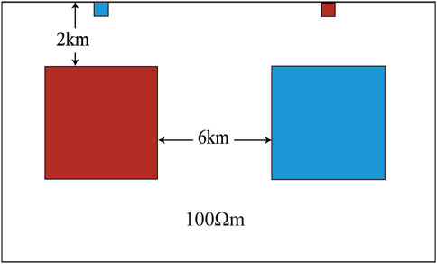
Figure 1. Model I Schematic. The red anomaly body has a resistivity of 10 Ω m, while the blue anomaly body has a resistivity of 1,000 Ω m. The edge length of the shallow anomaly body is 4 m, and the edge length of the deep anomaly body is 6 km.

The apparent resistivity profile obtained from forward modeling for Model 1 is shown on the Figure 2A. After removing the small anomalous bodies from the surface while keeping other conditions unchanged, the apparent resistivity profile obtained from forward modeling is shown on Figure 2B. In Figure 2A, some sites exhibit static shift, which appear as steep stripes in the profile. Static shift obscures the original subsurface structure and complicate data interpretation. In contrast, the phase profile (Figure 3) does not exhibit such situation. After the removal of apparent resistivity data containing static shift, the effect of static shift in the profile is significantly reduced, as shown in Figure 4. This reduction provides justification for using phase inversion without the need for static shift correction.

Figure 2

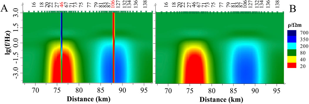
Figure 2. The TM apparent resistivity profile for model I (A) and model I without small anomalous bodies (B). The numbers at the top of the image represent the measurement site names, though not all measurement site names are displayed. The red numbers indicate measurement sites with static shifts (the same applies hereafter).

Figure 3

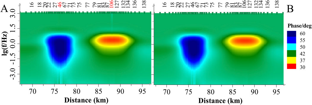
Figure 3. The TM phase profile for model I and model I (A) without small anomalous bodies (B).

Figure 4

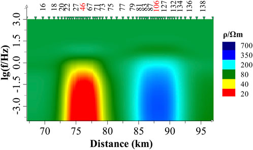
Figure 4. The TM apparent resistivity profile with apparent resistivity data excluded at affected sites.

In the forward modeling results, a random error of 10% was added to simulate measurement errors typically found in actual data. The inversion regularization factor was set to 100, with an initial model representing a homogeneous half-space of 100 $\mathrm{\Omega }\mathrm{m}$. The floor error for apparent resistivity was set at 2%, and the phase was established at 0.57°. Sparse inversion sites were employed, with neighboring sites spaced about 5 km apart. Four different inversion scenarios were conducted: (1) inversion using the original data, (2) inversion after static shift correction, (3) inversion based on the original data with the apparent resistivity data from static shift sites discarded, and (4) inversion after discarding both the apparent resistivity and phase data from static shift sites. In the static shift correction process, the TM curve was shifted to align with the high-frequency portion of the TE curve.

All four scenarios underwent multiple inversions, with the best inversion results selected for each case. The final inversion results are shown in Figure 6, where sites 46 and 106, located above the small anomalous bodies on the surface, are identified as static shift sites.

During the inversion process, the model is more inclined to closely align with the apparent resistivity curve compared to the phase curve. As demonstrated in Figure 5A with static shift site 106 as a reference, the inversion results closely replicate the displaced apparent resistivity data, yet exhibit a slightly inferior fit to the phase data, attributed to the influence of static shift. Following the application of static shift correction, as depicted in Figure 5B, the inversion results accurately align with both the apparent resistivity and phase data once the apparent resistivity curve is restored to its expected state. Figure 5C illustrates the inversion outcomes after the exclusion of the apparent resistivity data from the static shift site 106, revealing a good fit to the phase curve. Given that static shift does not impact the phase curve, the inversion results based on phase curve fitting for static shift sites are more representative of the true model than those derived from fitting the apparent resistivity curve.

Figure 5

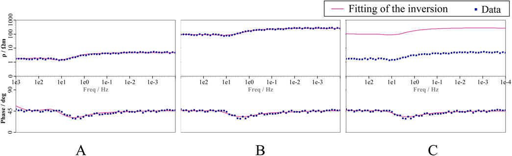
Figure 5. The fitting of measurement site 106 with frequency in the inversion results using different data. (A) Original data. (B) Date after static shift correction. (C) Original data with the apparent resistivity data from static shift sites discarded.

The inversion results using the original data are shown in Figure 6A. Due to static shift, two large anomalous bodies appear in the shallow region, while the deep low-resistivity anomaly is exaggerated, causing notable distortions in position, shape, and size. Additionally, the high-resistivity anomaly is obscured and unrecognizable. Figure 6B demonstrates that applying curve-shifting method yields excellent results, producing a smoother near-surface region and clearly distinguishable deep anomalies. Figure 6C closely resembles Figure 6B, indicating that, for this two-dimensional model, excluding the apparent resistivity data from static shift sounding sites can achieve results comparable to static shift correction. However, when phase data from static shift sites are also excluded, the lack of phase constraints results in blurred anomaly shapes and significantly deteriorates inversion quality (Figure 6D). This outcome underscores the critical role of phase data in the inversion process.

Figure 6

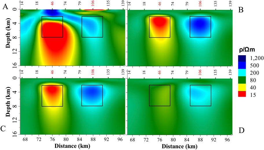
Figure 6. The results of inversion using different data. The black wireframe represents the location of the anomalous body. (A) Original data. (B) Date after static shift correction. (C) Original data with the apparent resistivity data from static shift sites discarded. (D) Discarding both the apparent resistivity and phase data from static shift sites.

4.2 3d/2d model

To further verify the reliability of this strategy, a 3D/2D model developed by Cai Juntao was utilized, with a schematic diagram shown in Figure 7 (Model II). This model was previously used in research by Cai and Chen (2010) on impedance tensor decomposition and structural dimensionality analysis.

Figure 7

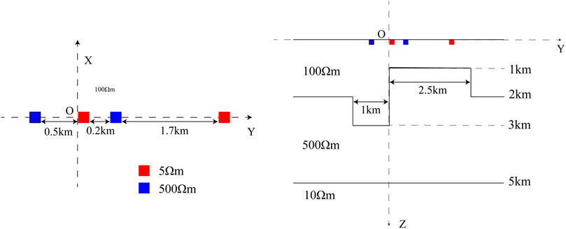
Figure 7. Model II Schematic. The 3D shallow heterogeneities are all cubic in shape with an edge length of 40 m (Cai, 2009).

The model surface contains four anomalous bodies, each measuring 40 m × 40 m × 40 m, with two high-resistivity bodies (500 $\mathrm{\Omega }\mathrm{m}$) and two low-resistivity bodies (5 $\mathrm{\Omega }\mathrm{m}$). The forward modeling spans a frequency range from 500 Hz to 0.0005 Hz, covering a total of 45 frequency points. Following the 3D forward modeling, data from survey lines intersecting the surface anomalies are selected for 2D inversion analysis.

Four different inversion scenarios were conducted: inversion using the original data directly, inversion after two different modes of static shift correction, and inversion after removing the apparent resistivity data from static shift measurement sites.

To implement the static shift corrections, the first correction involved shifting the TM curve to align with the TE curve using the initial branch merging method. The second correction involved globally shifting the TM curve to align its high-frequency section with the background resistivity value of 100 $\mathrm{\Omega }\mathrm{m}$ for the near-surface region in the forward model.

In all four scenarios, the regularization factor for inversion was set to 100. The initial model is a homogeneous half-space with a resistivity of 10 $\mathrm{\Omega }\mathrm{m}$. The synthetic data used for inversion included a random error of 10%. To obtain more accurate information about the deep structures, the impressing method (Ye et al., 2013) was employed to construct the initial model during the inversion process.

Furthermore, the best inversion results for each scenario were selected, and the final inversion results are presented in Figure 8. Additionally, when the small surface anomalies in the model were removed while keeping other conditions unchanged, the inversion results obtained after forward modeling are shown in Figure 9.

Figure 8

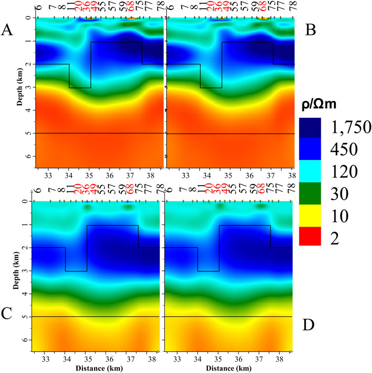
Figure 8. The inversion results of Model II. The black wireframe represents the layered structure. (A) Original data. (B) First time using static shift correction. (C) Second time using static shift correction. (D) Removing the apparent resistivity data from static shift site.

Figure 9

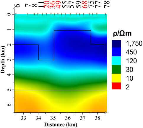
Figure 9. The inversion results of Model II without small anomalous bodies.

By comparing Figures 8, 9, it can be observed that Figure 8A exhibits near-surface anomalies that are not actually present due to static shift, particularly around the three small anomalies. A similar situation is noted in Figure 8B, where the shallow parts of both inversion results display significant irregularities. This indicates that when the model is three-dimensional, using TE apparent resistivity curve as a reference for curve translation is ineffective. However, Figure 8C shows that with a sufficient understanding of the electrical structure of the survey area, translating the TM curve to an appropriate value can yield improved inversion results. The results from the phase inversion of static shift sites in Figure 8D is similar to those in Figure 8C and closely resemble Figure 9.

Furthermore, static shift also causes a significant discrepancy in the position of the intermediate high-resistivity layer in the inversion results compared to the forward model, which is improved in Figures 8C, D. This indicates that the effects of static shift have been effectively suppressed, demonstrating that the proposed inversion strategy works well in three-dimensional situations.

It should be noted that the inversion results shown in Figures 8, 9 do not accurately reflect the deep information of the model. This is primarily due to inadequacies in the constructed mesh model for the forward modeling, which were necessary to accommodate the mesh division of the four small anomalies, resulting in significant errors in the low-frequency part of the synthetic data. To address this, a 2D model similar to Model II was designed, both with and without small surface anomalies. The results from the two-dimensional forward modeling and inversion of the synthetic data are shown in Figure 10, which better reflects the deep information of the model.

Figure 10

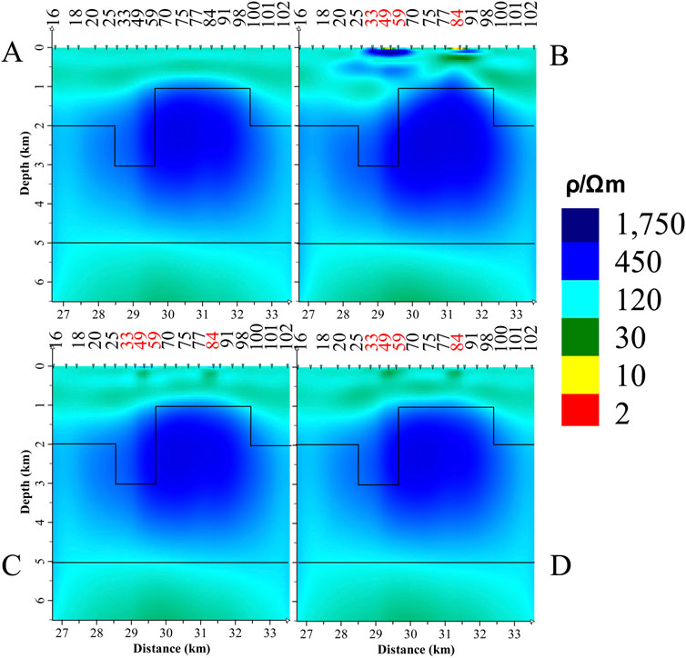
Figure 10. Inversion results of a 2D model similar to Model II. (A) Results for the 2D model without small anomalous bodies. (B) Inversion results for the original data. (C) Inversion results after static shift correction. (D) Inversion results excluding apparent.

4.3 Field test

A survey line in a specified area includes 28 sounding sites. Analysis revealed that site 51 exhibit static shift. Figure 11 displays the apparent resistivity profile along this line, where a vertical high-resistivity band appears between site 51. Removing the apparent resistivity data at this site significantly diminishes the effect of this vertical high-resistivity band. In the corresponding phase section diagram (Figure 12), no similar high-resistivity band was observed. Therefore, along this survey line, we can continue to attempt to use the inversion method proposed in this paper.

Figure 11

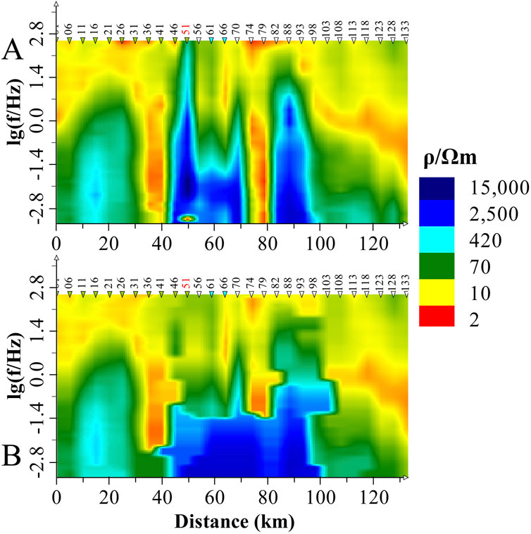
Figure 11. The TM apparent resistivity profile. (A) Original field data. (B) The apparent resistivity data excluded at affected site.

Figure 12

Figure 12. The TM phase profile for field data.

Two inversions were performed: one including the apparent resistivity data for site 51 and another excluding it. The results are shown in Figure 13. Overall, the difference between the two inversions is minor, indicating that for 2D field data, the effect of static shift on inversion results is less pronounced than in theoretical model inversions. However, some localized distortions remain. At the 40 km mark along the line, a high-resistivity anomaly approximately 2 km deep and 8 km thickness distorts the shapes of adjacent low-resistivity anomalies, impacting the visibility of high-conductivity zones and potentially influencing geological interpretations (represented by black rectangles in Figure 13). After discarding the apparent resistivity data from static-shift-affected sites and conducting the inversion, the resistivity variations in this region become smoother, aligning more closely with the true resistivity values.

Figure 13

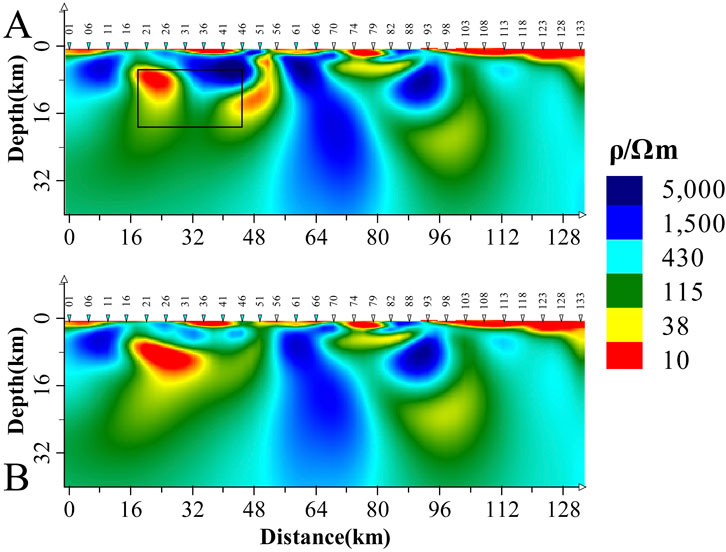
Figure 13. Results of Field Data Inversion. (A) Inversion results for the original data. (B) Inversion results for the original data with apparent resistivity data from static shift sites removed.

5 Discussion

In magnetotellurics, in addition to small surface anomalies, there are other situations, such as steep terrain, vertical fractures that cut through to the surface, and boundaries between rocks with different properties, which can also cause shifts in the apparent resistivity curve. If these factors are not properly identified, blindly applying static shift correction can easily remove data that accurately reflects the structural response. The aforementioned cases illustrate that this can have a severe impact on inversion results. Therefore, it is crucial to determine whether a measurement site is affected by static shift. Currently, static shift identification primarily relies on experience, which means there is a possibility of misidentification. When a measurement site without static shift is mistakenly identified as having static shift, which method would have a greater impact: the traditional static shift correction method or the direct discard of apparent resistivity advocated in this paper?

Figure 14 presents several inversion results based on the inversion outcome shown in Figure 6C. Assuming that measurement site 74 is misjudged as having a static shift, Figures 14B, C show the inversion results with static shift correction factors set to 5 and 0.2, respectively, while Figure 14D shows the inversion result after discarding the apparent resistivity data of measurement site 74. All other inversion parameters remain consistent with those in Figure 6.

Figure 14

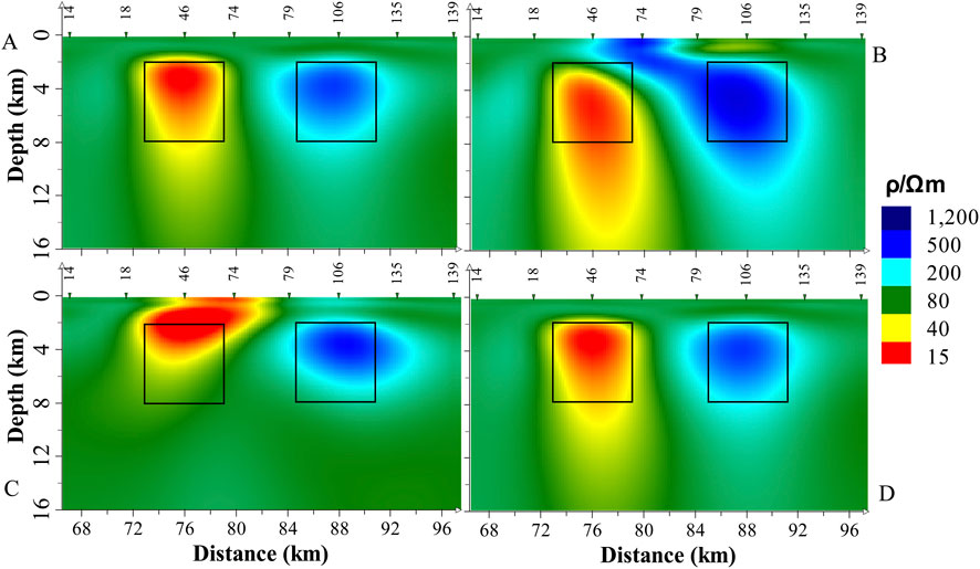
Figure 14. The inversion results for Model (I) (A) Apparent resistivity data from two measurement sites affected by static shift are discarded, consistent with Figure 6C; (B) Static shift correction factor for measurement site 74 is 5; (C) Static shift correction factor for measurement site 74 is 0.2; (D) The apparent resistivity data for measurement site 74 is discarded.

It is clear that, after misjudgment, the traditional method of static shift correction by shifting the apparent resistivity, whether moving it upwards (Figure 14B) or downwards (Figure 14C), significantly impacts the inversion results. The upward shift (Figure 14B) causes a particularly severe distortion, likely because increasing the apparent resistivity creates high-resistivity anomalies, which in turn increases the skin depth of electromagnetic waves, resulting in a larger impact range of erroneous data. In contrast, the method proposed in this paper (Figure 14D), which involves simply excluding the apparent resistivity data of measurement site 74 from the inversion, causes negligible effects on the inversion result, with only a slight downward extension of the bottom boundary of the high-conductivity anomaly.

The same testing and processing were applied to the field data in this paper. Suppose that measurement site 26 on this profile is misjudged as a static shift site, and after applying various static shift corrections, the inversion results are compared as shown in Figure 15. From Figure 15, it can be seen that the error correction of the misjudged static shift in this field data case is not as significant as in Figure 14, but differences are still observable. When the apparent resistivity curve of measurement site 26 is multiplied by a static shift factor of 0.2, the result, shown in Figure 15B, differs slightly from Figure 15A. However, it is still evident that R1 has become notably narrower, and the scales of R2 and C have also decreased. If the apparent resistivity curve of measurement site 26 is multiplied by a static shift factor of 5, the result, shown in Figure 15C, shows a much more obvious difference compared to Figure 15A. R1 has significantly thickened, the burial depth of the top boundary of C has increased substantially, and its shape has also changed, while R2 is less affected. However, by directly excluding the apparent resistivity data of measurement site 26 from the inversion, as done in this paper, the result, shown in Figure 15D, indicates that the difference between it and Figure 15A is mainly in the continuity between measurement sites 26 and 31 in R1, which now appears more continuous, reflecting the smallest variation among the three sites.

Figure 15

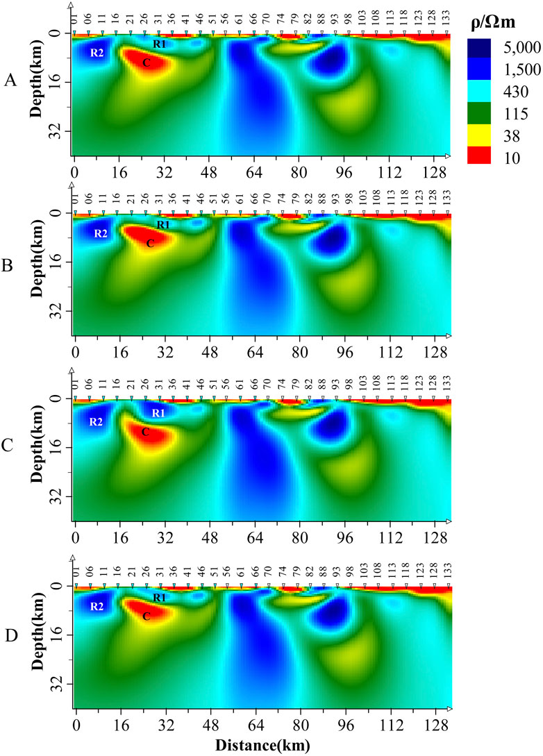
Figure 15. The inversion results for field data, R1, R2, and C represent the anomaly bodies. (A) The inversion result after excluding the apparent resistivity data of measurement site 51, consistent with Figure 13B; (B) Static shift correction factor of 0.2 applied to measurement site 26; (C) Static shift correction factor of 5 applied to measurement site 26; (D) The apparent resistivity data of measurement site 26 is excluded.

Both the theoretical model and the field data case demonstrate that, when a static shift site is misjudged, traditional methods have a larger impact on the inversion results compared to the method proposed in this paper. Specifically, shifting the apparent resistivity upward has a much greater impact on the inversion results than shifting it downward by the same factor. In the field data case in this paper, the correction of the misjudged static shift site has a relatively small effect on the inversion results (similar to synthetic data). This may be due to the presence of a significant high-conductivity anomaly (C) beneath the measurement site, which causes the electromagnetic wave to attenuate rapidly inside, limiting the propagation of the static shift effect to more distant areas, thus reducing the range of influence.

The above examples preliminarily suggest that if static shift measurement sites are misidentified, specifically when a measurement site without static shift effects is incorrectly determined to have a static shift, the impact of the traditional processing method is far greater than that of the method proposed in this paper. The reason for the smaller impact of the proposed method is that the information contained in the discarded apparent resistivity data can be recovered through the retained phase data and the apparent resistivity data from neighboring measurement sites. After all, both 2D and 3D inversions are collaborative processes involving multiple measurement sites to reconstruct the subsurface electrical structure. Of course, if multiple measurement sites are misjudged and too much apparent resistivity data is discarded during inversion, leading to insufficient data constraints on the electrical structure background of the survey area, the inversion results will be affected. The specific impact of this scenario requires further investigation.

6 Conclusion

This study investigates the influence of static shift on magnetotelluric data by analyzing the inversion results of both two-dimensional and three-dimensional models, as well as field data. This analysis raises a critical question: Is static shift correction necessary for every MT project? Our findings indicate that static shift correction is not an obligatory procedure in MT.

By utilizing phase data from static shift sites as the primary input for inversion, this strategy effectively reduces subjective operator bias, provided that the static shift sites are accurately identified. Additionally, this method is straightforward and does not incur additional observational costs compared to traditional static shift correction techniques. Consequently, this inversion strategy successfully mitigates the effects of static shift in the data without increasing the expenses associated with MT data acquisition or complicating data processing workflows. This approach not only addresses the challenges posed by static shift effects on inversion results but also enhances the overall reliability of these results.

This study has limitations, including the omission of topographical effects and a lack of validation through three-dimensional inversion, based on the assumption that the forward modeling results of the theoretical model are sufficiently accurate. While various two-dimensional models were designed and validated throughout the research process, producing generally satisfactory results, actual subsurface electrical structures are often far more complex. Thus, further theoretical and practical investigations are necessary to substantiate these findings in this domain.

Data availability statement

The raw data supporting the conclusions of this article will be made available by the authors, without undue reservation.

Author contributions

JZ: Investigation, Validation, Visualization, Writing - original draft, Writing - review and editing, Data curation. XC: Conceptualization, Software, Supervision, Validation, Writing - review and editing, Funding acquisition, Methodology, Resources. PW: Software, Validation, Visualization, and Writing – review and editing. ZL: Investigation, Writing - review and editing, Validation. JC: Resources, Writing - review and editing.

Funding

The author(s) declare that financial support was received for the research, authorship, and/or publication of this article. This work is supported by the National Natural Science Foundation of China (42174093) and Three-Dimensional Electrical Structure of the Central and Northern Segment of the Red River Fault Zone (ZDJ 2020-13).

Conflict of interest

The authors declare that the research was conducted in the absence of any commercial or financial relationships that could be construed as a potential conflict of interest.

Generative AI statement

The author(s) declare that Generative AI was used in the creation of this manuscript. Optimized English expression.

Publisher’s note

All claims expressed in this article are solely those of the authors and do not necessarily represent those of their affiliated organizations, or those of the publisher, the editors and the reviewers. Any product that may be evaluated in this article, or claim that may be made by its manufacturer, is not guaranteed or endorsed by the publisher.

References

Beamish, D., and Travassos, J. M. (1992). A study of static shift removal from magnetotelluric data. J. Appl. Geophys. 29 (2), 157–178. doi:10.1016/0926-9851(92)90006-7

CrossRef Full Text | Google Scholar

Berdichevsky, M. N., Dmitriev, V. I., and Pozdnjakova, E. E. (1998). On two-dimensional interpretation of magnetotelluric soundings. J. Geophys. Res. Solid Earth 133, 585–606. doi:10.1046/j.1365-246X.1998.01333.x

CrossRef Full Text | Google Scholar

Bostick, F. X. (1986). Electromagnetic array profiling (EMAP). SEG Technical Program Expanded Abstracts: 60–61. doi:10.1190/1.1892989

CrossRef Full Text | Google Scholar

Cagniard, L. (1953). Basic theory of the magneto-telluric method of geophysical prospecting. Geophysics 18, 605–635. doi:10.1190/1.1437915

CrossRef Full Text | Google Scholar

Cai, J., Chen, X., Xu, X., Tang, J., Wang, L., Guo, C., et al. (2017). Rupture mechanism and seismotectonics of the _s6.5 Ludian earthquake inferred from three-dimensional magnetotelluric imaging. Geophys. Res. Lett. 44, 1275–1285. doi:10.1002/2016GL071855

CrossRef Full Text | Google Scholar

Cai, J. T. (2009). Research on the three-dimensional distortion characteristics and correction techniques of magnetotelluric data [Doctoral dissertation]. China Earthquake Administration: Institute of Geology.

Google Scholar

Cai, J. T., and Chen, X. B. (2010). Refined techniques for data processing and two-dimensional inversion in magnetotelluric II: which data polarization mode should be used in 2D inversion. Chin. J. Geophys. 53 (11), 2703–2714. doi:10.3969/j.issn.0001-5733.2010.11.018

CrossRef Full Text | Google Scholar

Calderón-Moctezuma, A., Gomez-Treviño, E., Yutsis, V., Guevara-Betancourt, R., and Gómez-Ávila, M. (2022). How close can we get to the classical magnetotelluric sounding? J. Appl. Geophys. 203, 104665. doi:10.1016/j.jappgeo.2022.104665

CrossRef Full Text | Google Scholar

A. D. Chave, and A. G. Jones (2012). The magnetotelluric method: theory and practice (Cambridge University Press CUP). doi:10.1017/CBO9781139020138

Chen, X. B., and Hu, W. B. (2002). Direct iterative finite element (DIFE) algorithm and its application to electromagnetic response modeling of line current source. Chin. J. Geophys. 45 (01), 119–130. doi:10.1002/cjg2.223

CrossRef Full Text | Google Scholar

Chen, X. B., Zhao, G. Z., and Ma, X. (2006). Study on the 1D and 2D inversion approximation problems of magnetotelluric three-dimensional models. Chin. J. Eng. Geophys., 9–15.

Google Scholar

Chen, X. B., Zhao, G. Z., and Zhan, Y. (2004). MT data processing and interpretation Windows-based visualization integration system. Pet. Geophys. Prospect. 39 (S1), 11–16.

Google Scholar

Duan, B. (1994). First branch recombination method for correcting static effects in magnetotelluric sounding. J. Changchun Coll. Geol., 444–449.

Google Scholar

Fischer, G., and Schnegg, P.-A. (1980). The dispersion relations of the magnetotelluric response and their incidence on the inversion problem. Geophys. J. Int. 62, 661–673. doi:10.1111/j.1365-246X.1980.tb02598.x

CrossRef Full Text | Google Scholar

Gao, H., and Zhang, S. (1998). Study of correction for static shift: the decomposition of magnetotelluric impedance tensors. Geol. Sci. Technol. Inf. 17(1), 91–96.

Google Scholar

Groom, R. W., and Bailey, R. C. (1989). Decomposition of magnetotelluric impedance tensors in the presence of local three-dimensional galvanic distortion. J. Geophys. Res. Solid Earth 94, 1913–1925. doi:10.1029/JB094iB02p01913

CrossRef Full Text | Google Scholar

Guo, W., Tang, X. G., and Sheng, G. Q. (2022). Magnetotelluric static correction of two-dimensional model based on the highest frequency phase method and spatial filtering method. Acta Seismol. Sin. 44 (2), 302–315. doi:10.11939/jass.20210139

CrossRef Full Text | Google Scholar

Jiang, F., Chen, X., Unsworth, M. J., Cai, J., Han, B., Wang, L., et al. (2022). Mechanism for the uplift of gongga Shan in the southeastern Tibetan plateau constrained by 3d magnetotelluric data. Geophys. Res. Lett. 49, e2021GL097394. doi:10.1029/2021GL097394

CrossRef Full Text | Google Scholar

Jiracek, G. R. (1990). Near-surface and topographic distortions in electromagnetic induction. Surv. Geophys. 11 (2-3), 163–203. doi:10.1007/BF01901659

CrossRef Full Text | Google Scholar

Jones, A. G. (2012). Static shift of magnetotelluric data and its removal in a sedimentary basin environment. Geophysics 53, 967–978. doi:10.1190/1.1442533

CrossRef Full Text | Google Scholar

Luo, Y. Z., He, Z. X., Ma, R. W., and Guo, J. H. (1991). The correction of static effects in sonic-frequency telluric electromagnetic method of controllable source. Geophys. Geochem. Explor., 196–202.

Google Scholar

Luo, Z. Q. (1990). Study on suppressing the effect of static shift in MT by electromagnetic array profiling method. J. China Univ. Geosciences, 13–22.

Google Scholar

Qiu, G., Zhong, Q., Liu, J., Bai, D., and Yuan, Y. (2012). Approximate interconversion method and program implementation between apparent resistivity and phase curves in magnetotelluric sounding. Comput. Tech. For Geophys. And Geochem. Explor. 34, 402–405+366.

Google Scholar

Rodi, W., and Mackie, R. L. (2001). Nonlinear conjugate gradients algorithm for 2-D magnetotelluric inversion. Geophysics 66, 174–187. doi:10.1190/1.1444893

CrossRef Full Text | Google Scholar

Sasaki, Y. (2004). Three-dimensional inversion of static-shifted magnetotelluric data. Earth Planets Space 56, 239–248. doi:10.1186/BF03353406

CrossRef Full Text | Google Scholar

Song, S., Tang, J., and He, J. (1995). Wavelets analysis and the recognition, separation, and removal of the static shift in electromagnetic soundings. Chin. J. Geophys. 38 (1), 120–128.

Google Scholar

Spitzer, K. (2001). Magnetotelluric static shift and direct current sensitivity. Geophys. J. Int. 144, 289–299. doi:10.1046/j.1365-246x.2001.00311.x

CrossRef Full Text | Google Scholar

Sternberg, B. K., Washburne, J. C., and Pellerin, L. (1988). Correction for the static shift in magnetotellurics using transient electromagnetic soundings. Geophysics 53, 1459–1468. doi:10.1190/1.1442426

CrossRef Full Text | Google Scholar

Tikhonov, A. N. (1950). On determining electric characteristics of the deep layers of the Earth’s crust. Dokl. Akad. Nauk. SSSR 73.

Google Scholar

Trad, D. O., and Travassos, J. M. (2012). Wavelet filtering of magnetotelluric data. Geophysics 65, 482–491. doi:10.1190/1.1444742

CrossRef Full Text | Google Scholar

Tripaldi, S., Siniscalchi, A., and Spitzer, K. (2010). A method to determine the magnetotelluric static shift from DC resistivity measurements in practice. Geophysics 75, F23–F32. doi:10.1190/1.3280290

CrossRef Full Text | Google Scholar

Wang, J. Y. (1990). Basic principles of the electromagnetic array profiling method. Earth Sci. J. China Univ. Geosciences S1, 1–11.

Google Scholar

Wang, J. Y. (1992). On the issue of static correction in magnetotellurics. Geol. Sci. Technol. Inf. 11, 69–76.

Google Scholar

Wang, J. Y. (1997). New development of magnetotelluric sounding in China. Chin. J. Geophys. 40 (S1), 206–216.

Google Scholar

Wang, S. (1998). The correction of magnetotelluric curve distortion caused by surficial local three-dimension inhomogeneities: the impedance tensor decomposition technique for the correction of MT curves distortion. Northwest. Seismol. J. 20 (4), 1–11.

Google Scholar

Wannamaker, P. E., Hohmann, G. W., and Ward, S. H. (1984). Magnetotelluric responses of three-dimensional bodies in layered earths. Geophysics 49, 1517–1533. doi:10.1190/1.1441777

CrossRef Full Text | Google Scholar

Yang, J., Xiao, H. Y., Jiang, Y. D., and Yang, W. (2015). Research and application of several static shift correction methods for magnetotelluric sounding data. Comput. Tech. Geophys. Geochem. Explor. 37, 187–192.

Google Scholar

Yang, S., Bao, G. S., and Zhang, S. Y. (2001). Correction of distorted apparent resistivity curves using impedance phase data in MT method. Geol. Prospect. 37, 42–45.

Google Scholar

Ye, T., Chen, X., and Yan, L. (2013). Refined techniques for data processing and two-dimensional inversion in magnetotellurics (VII): electrical structure and seismogenic environment of Yingjiang-Longling seismic area. Chin. J. Geophys. 56 (10), 3596–3606. doi:10.6038/cjg20131034

CrossRef Full Text | Google Scholar

Zhang, K., Yan, J., Cai, D., Wei, W., Qu, S., Tang, B., et al. (2016). A joint magnetotelluric field static shift 2D correction method and its application. Earth Sci. 41 (5), 864–872. doi:10.3799/dqkx.2016.073

CrossRef Full Text | Google Scholar

Zhang, X. (1999). Identifying apparent polarized resistivity curves of TE and TM mode from magnetotelluric sounding. J. Oil Gas Technol. 21 (4), 72–75. doi:10.3969/j.issn.1000-9752.1999.04.026

CrossRef Full Text | Google Scholar

Zhang, X., Hu, W., Yan, L., and Zhang, S. (2002). Application of wavelet transform in the static correction of magnetotelluric sounding. J. Jianghan Petroleum Inst. 24, 40–41.

Google Scholar