Design of precise fertilization method for greenhouse vegetables based on improved backpropagation neural network

The traditional method of detecting crop nutrients is based on the direct chemical detection method in the laboratory, which causes great damage to crops. In order to solve the above problems, the main goal of this study is to design a precise fertilization method for greenhouse vegetables based on the improved back-propagation neural network (IM-BPNN) algorithm to increase fertilizer utilization efficiency, reduce production costs, and improve the economic viability of agriculture. First, soil samples from the farm in china are selected. With the laboratory treatment, available phosphorus, available potassium, and alkaline nitrogen are extracted. These data are preprocessed by the z-score (zero-mean normalization) standardization method. Then, the BPNN (backpropagation neural network) algorithm is improved by being trained and combined with the characteristics of the dual particle swarm optimization algorithm. After that, the soil sample data are divided into training and test sets, and the model is established by setting parameters, weights, and network hierarchy. Finally, the NBTY (nutrient balance target yield),BPNN (backpropagation neural network) and IM-BPNN algorithm are used to calculate the amount of fertilizer. Compared with the BPNN and NBTY algorithm, it shows that the IM-BPNN algorithm can more accurately determine the amount of fertilizer required by vegetables and avoid over-application, which can improve fertilizer utilization efficiency, reduce production costs, and improve the economic feasibility of agriculture.

1 Introduction

The reasonable crop nutrient supply is of great significance to the healthy growth of crops, especially nitrogen, phosphorus, and potassium, which is the most important nutrient elements for crop growth in china. However, existing fertilization methods are mainly based on manual decision-making, which is easily affected by factors such as subjective judgment, experience bias, and insufficient information. Moreover, the lack of comprehensive and accurate soil and plant information makes the fertilization plan easily deviate from the optimal state, which reduces useful efficiency of nutrient and increases the waste of agricultural resources (Youlu, 2018). Although some methods for accurately detecting crop nutrients are based on the direct chemical detection methods in the laboratory, some of which are at the cost of the survival and growth of crops, and meanwhile with the disadvantages of poor real-time performance, high cost, and large pollution. Therefore, how to apply artificial intelligence technology to crop growth has become a current research hotspot, with scientific and efficient fertilization the focus of research, which is benefited to the development of precision fertilization (Sharma et al., 2023).

In order to solve the above problems, some scholars made some achievements in the fertilization decision-making systems. Jin et al. (2020) designed an intelligent monitoring system for vegetable fertilization and sowing. It uses GPS and soil prescription plot maps to determine the target amount of fertilizer, and uses pressure sensors and microcomputer control to calculate the amount of fertilizer and flow information. Shamshiri et al. (2020) proposed a novel comfort ratio model connected with IoT sensors to evaluate greenhouse microclimate parameters. He also developed an optimization algorithm for set point manipulation in microclimate control. Dong et al. (2020) proposed a method for precise fertilization of field crops based on a wavelet-BP neural network. It combines wavelet analysis with BP neural network to analyze the complex non-linear relationship between soil nutrients, fertilizer application and crop yield, which can improve the prediction accuracy of the model. Coulibali et al. (2020) proposed a site-specific machine learning predictive fertilization model for potato crops in eastern Canada. It uses machine learning algorithms to determine an optimal model for predicting high tuber yield and quality. Swaminathan et al. (2023) proposed a deep neural collaborative filtering model for fertilizer prediction. It uses feature fusion and deep learning technology to effectively capture the complex interactive relationship between soil and fertilizer, which improve the accuracy of the algorithm in predicting the amount of fertilizer. Shamshiri et al. (2018) proposed a method for evaluating and controlling microclimate in greenhouse tomato cultivation based on optimal temperature, humidity and vapor pressure difference. It defines the membership function model of the optimality of the optimal, critical and failed air and root zone temperatures of tomatoes to determine the optimal growth conditions of tomatoes.

Zhang et al. (2019) designed a QUEFTS model to estimate the nutrient absorption requirements of radish in China. It used the Quantitative Evaluation of Tropical Soil Fertility (QUEFTS) model to study the relationship between radish fleshy root yield and nutrient accumulation, and obtained the optimal balanced requirements of N, P and K for radish plants to produce 1,000 kg of fleshy roots. Brunetto et al. (2022) used a machine learning model to predict nitrogen use in the “Alicante Bouschet” vineyard. They conducted a 5-year fertilization experiment and used ML tools to build a model including nitrogen dosage, climate index, foliar nitrogen dosage, and stem diameter of the previous season to achieve nitrogen management from local characteristics. Recena et al. (2019) used the visible–near infrared spectroscopy (Vis–NIR) to find the response sites of P, Ca, Mg, K and Fe in vegetable soils, which accurately estimated the plant-available phosphorus and potassium content in crops, and control the application of phosphorus and potassium fertilizers. Shamshiri et al. (2021) proposed a wireless sensor and IoT instrument integrated with artificial intelligence to realize greenhouse automation process. It is equipped with a distributed wireless node custom-designed based on a powerful dual-core 32-bit microcontroller to achieve optimal growth conditions and automatic fertilization of greenhouse crops. Ashraf et al. (2021) proposed a Maisotsenko cycle evaporative cooling (M-DAC) system based on desiccant dehumidification. It optimizes the traditional greenhouse air conditioning system from the perspective of temperature gradient, relative humidity level, VPD and dehumidification gradient, so that crops can grow in the best environmental conditions. Rezvani et al. (2021) proposed a greenhouse crop growth simulation model based on energy balance and computational fluid dynamics to balance the relationship between climate, soil, water and crops to achieve optimal growth of crops.

Although the above studies provide fertilization decisions based on some crops, some of these studies need to focus on the convergence of the algorithm, computational efficiency and the use of large-scale data sets, and the practicability of the algorithm in actual farm applications is not high. Some studies requires the use of infrastructure (such as greenhouse climate constant temperature system, GIS systems, etc.), but these equipment are expensive, which may impose an economic burden on small farms. Finally, some fertilization decision-making methods involve multiple variables, including soil texture, plant varieties, meteorological conditions, etc. There are uncertainties and inaccuracies in these data, which may affect the accuracy of fertilization decisions, and the above methods are not practical in practice. The applications are relatively complex and limited by hardware equipments and network infrastructures. Although Junfeng et al. (2022) proposed to predict the impact of different application amounts of nitrogen, phosphorus and potassium on the tomato yield and quality in solar greenhouses of the Gobi region, this method is limited by specific geographical and climatic conditions, so it has the versatility of greenhouse agriculture. In order to solve the above problems, the main goal of this study is to develop a precise fertilization method for greenhouse vegetables based on the improved back-propagation neural network (IM-BPNN) algorithm to improve the accuracy of fertilization, thereby improving fertilizer utilization efficiency and reducing agricultural production costs. By introducing the double particle swarm optimization algorithm, this method aims to improve the accuracy of the BPNN algorithm in determining the amount of fertilizer required for vegetables, thereby achieving high yield and efficiency.

2 Materials and methods

2.1 Algorithm design

In this study, the dual particle swarm algorithm was introduced to the BP neural network, which was combined to improve the algorithm’s accuracy (Qiuying, 2017).

2.1.1 Backpropagation neural network

Backpropagation Neural Network (BPNN) is a multi-layer feedforward neural network used for classification and regression tasks (Gunawan et al., 2022). It learns and adjusts the weights of the network through two stages of forward propagation and back propagation to minimize the prediction error. As to the forward propagation, the nodes of the input layer receive the input data and pass it to the hidden layer; each node of the hidden layer weights the input data Sum and perform a nonlinear transformation through an activation function (such as the Sigmoid function), and then pass the result to the next layer. The nodes of the output layer receive the output of the hidden layer, perform weighted summation and activation function transformation, and finally output the predicted value. As to the backpropagation, it calculates the error between the predicted value and the actual value of the output layer, makes the error from the output layer to the hidden layer, and calculates the error gradient of each node. Finally, according to the error gradient, the weights and biases of nodes in each layer of the network are adjusted to gradually reduce the prediction error (Zhang et al., 2019). The BP neural network was trained according to the following steps:

(1) Initialization: the parameters such as the number, weight, neuron bias, and learning rate of each hidden layer node are set. Among them, Neuron Bias is an additional parameter. Its function is similar to the intercept term in linear regression and can help the model fit the data better. The existence of the bias term enables the activation function to be translated so that it is no longer limited to the vicinity of the origin, increasing the flexibility and expressiveness of the model. Activation Function is a nonlinear transformation between the output of each neuron in the neural network and its input. It is used to introduce nonlinearity so that the neural network can handle complex nonlinear problems. The learning rate is a hyperparameter that determines the size of the step size each time the model parameters are updated.

(2) Calculating the hidden layer output: the calculation of the hidden layer output is expressed as Formula 1:

$\begin{array}{ll}{G}_{\phi }=P\left({\displaystyle \sum }_{m=1}^i{a}_m\times u_{m\phi }-x_{\phi }\right)& (1)\end{array}$

In Formula 1, $\phi$ represents the number of the hidden layer node; $m$ represents the number of the input layer node; $i$ represents the total number of input layer nodes; $m\phi$ represents the input value of the mth input layer node; $G_{\phi }$represents the output of the $\phi -th$ node in the hidden layer; $P\left(\right)$ represents the activation function; $\mathrm{i}$ represents the number of input layer nodes; $u_{m\phi }$ represents the connection weight from the $m-th$ input layer node to the $\phi -th$ hidden layer node ( $\phi$ =1,2,…,j). Based on the data, the Sigmoid function is adopted as the activation function to build a real number to the (0, 1) interval, which is expressed as Formula 2:

$\begin{array}{ll}P\left(a\right)=1/\left(1+{\omega }^{-a}\right)& (2)\end{array}$

(3) Calculating the actual output: the real output is computed, $y_n$ represents the offset value (n = 1, 2,…, $\gamma$ .), which is shown in Formula 3:

$\begin{array}{ll}{R}_{\phi }={\displaystyle \sum }_{\phi =1}^j\left(H_{\phi }\times u_{n\phi }\right)-y_n& (3)\end{array}$

(4) Backpropagation: the error value is calculated by Formula 4:

$\begin{array}{ll}{w}_n=\overline{R_n}-R_n& (4)\end{array}$

Then the weight is updated, and the calculation of the updated weight from the input layer to the ahidden layer is expressed as Formula 5:

$\begin{array}{ll}{u}_{m\phi }=u_{m\phi }+G_{\phi }\times \left(\rho -\rho \times G_{\phi }\right)\times {\displaystyle \sum }_{n=1}^t\left(u_{n\phi }\times w_n\right)& (5)\end{array}$

In Formula 5, $\rho$ represents the learning rate. The updated weights from the hidden layer to the output layer is computed by Formula 6:

$\begin{array}{ll}{u}_{m\phi }=u_{m\phi }+\rho \times G_{\phi }\times w_n& (6)\end{array}$

Finally, the threshold is updated. The updated from the input layer to the hidden layer is computed by Formula 7:

$\begin{array}{ll}{x}_{\phi }=x_{\phi }+G_{\phi }\times \left(\rho -\rho \times G_{\phi }\right)\times {\displaystyle \sum }_{n=1}^t\left(u_{n\phi }\times w_n\right)& (7)\end{array}$

The updated threshold from the hidden layer to the output layer is computed by Formula 8:

$\begin{array}{ll}{y}_n=y_n+w_n& (8)\end{array}$

The BPNN algorithm transforms the input data to the output data through the activation function and continuously fit any nonlinear function through the backpropagation function, which is good adaptability and robustness. However, it has some disadvantages, such as slow convergence, easy to fall into local optimum, overfitting, etc. Therefore, it is necessary to integrate other algorithms to improve model accuracy and efficiency, so the dual particle swarm optimization algorithm can meet this requirement (Chen et al., 2019).

2.1.2 Dual particle swarm optimization algorithm

The duel particle algorithm upgrades the original particle swarm algorithm. It divides the particle swarm into two populations and uses different learning algorithms to identify the optimal value (Jain et al., 2020). Meanwhile, in order not to completely abandon the discarded particle information, the particle swarm is divided into the following two types:

For the main group, the method of linearly decreasing inertial weight ɷ is used for searching, and the genetic algorithm is combined to optimally preserve inheritance and small probability mutation to update the particles. Formulas 9 and 10 are as follows:

$\begin{array}{c}{C}_m\left(\alpha +1\right)=\mathrm{\epsilon }{C}_m\left(\alpha \right)+{\alpha }_1{\beta }_1\left(H{y}_n\left(k\right)-A_m\left(k\right)\right)\\ +{\alpha }_2{\beta }_2\left(D{y}_n\left(k\right)-A_m\left(k\right)\right)\end{array}\text{ (9)}$

$\begin{array}{ll}{A}_m\left(k+1\right)=A_m\left(k\right)+C_m\left(k+1\right)& (10)\end{array}$

In Formula 9, $C_m\left(\alpha +1\right)$ represents the velocity of the m-th particle in the α + 1th generation; $\mathrm{\epsilon }$ represents the inertial weight, which controls the search ability and development ability of particles. A larger inertia weight helps global search, while a smaller inertia weight helps local search; ${\alpha }_1$ and ${\alpha }_2$ represents the acceleration constant, which determines the acceleration of particles approaching the individual optimal position and the global optimal position, respectively. The value is [1,2] to ensure that particles can balance exploration and exploitation. ${\beta }_1$and ${\beta }_2$ represents a random number, with a value range of [0, 1]. Randomness is introduced to increase the diversity of the particle swarm and prevent it from falling into local optimality. $H{y}_n\left(k\right)$ represents the historical optimal position of the current particle, and $D{y}_n\left(k\right)$ represents the global optimal position of the particle swarm. They ensure that the particles move toward the historical best position and the current global optimal position, improving the optimization ability of the algorithm. $A_m\left(k\right)$ represents the current particle position.

In Formula 10, A represents the position of the m-th particle in the (k + 1)-th generation. B represents the position of the m-th particle in the k-th generation, which is the basis for the next position update. C represents the speed of the m-th particle in the (k + 1)-th generation, which determines the moving direction and distance of the particle in the next step. Through the speed and position updates of the above two formulas, the particle swarm can continuously adjust its position in the search space and finally converge to the global optimal solution. Since the main group uses the decreasing weight to search the later stage of iteration, the extreme value falls into the local value with the decrease of $\mathrm{\epsilon }$ , which is possible to filter out the particles of the global value. The auxiliary group consists of two parts: one part is the particles rejected from the main group, and the other is the particles randomly selected in the particle group. It is expressed by Formula 11:

$\begin{array}{ll}{H}_{2i}=\overline{H_i}\times 50\%+H_i\times 50\%& (11)\end{array}$

In Formula 11, $H_{2i}$ represents the position of the 2i-th particle in the new generation. $\overline{H_i}$ represents the position of the i-th particle in the current generation. $H_i$ represents the position of the i-th particle, which is selected from the other particles in the swarm. The main group and the auxiliary group account for 70 and 30% of the particle swarm. The two groups are calculated according to the above two points. During the iteration process, the auxiliary group keeps filtering particles, so the particles are overlaped with the main group, which are the optimal particles.

2.1.3 Improved backpropagation neural network

In order to improve the accuracy of the BPNN alogrithm, BP train and DPSO (Particle Swarm Optimization) class are defined. The population size of the particle swarm optimization algorithm is set as j, the maximum speed is $C_{\text{max}}$ , the inertia weight coefficient is w, the acceleration coefficients is ${\alpha }_1$ and ${\alpha }_2$ , the highest iteration number is m. The training set is passed into fit for training, the BP is used to construct the mathematical model. Finally, the output value of the neural units in each layer and the error rate between the output value and the real value are calculated to facilitate subsequent optimization of the algorithm using weights and deviations. The pseudocode of the IM-BPNN algorithm algorithm is as follows:

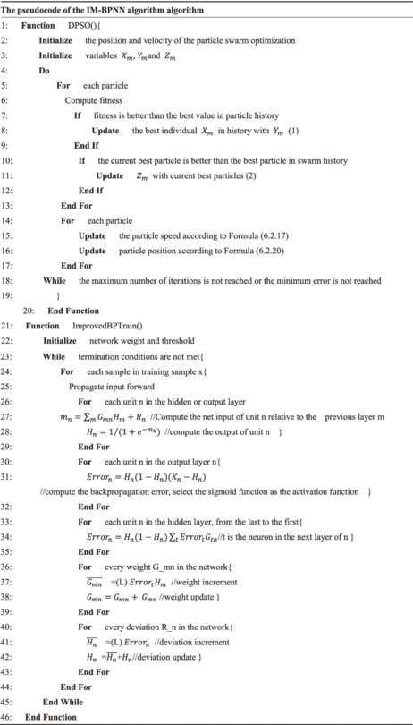
The process of the IM-BPNN algorithm is shown in Figure 1.

Figure 1

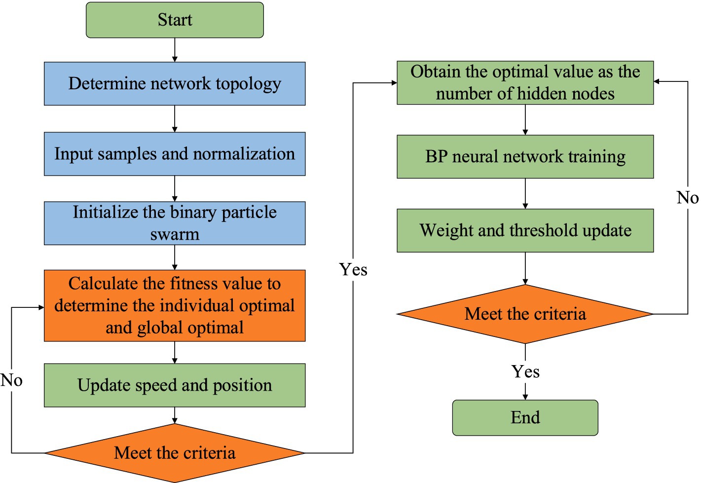
Figure 1. The process of the IM-BPNN algorithm.

2.2 Experimental design

2.2.1 Experimental environment

The study data is taken from the research area of a farm in Shuixi Village, Qingyuan, Guangdong, China, which covers up to 500 acres. The object of this study is Komatsuna. Figure 2 shows the komatsuna production environment and soil monitoring equipment. (a) It shows the vegetable agricultural production base, covered with a transparent greenhouse for protecting and growing vegetables. (b) It shows the pineapple planting area, which shows the planting area inside the greenhouse, with pineapple seedlings planted neatly in the soil. (c) It shows the vegetable soil tester, which is a soil testing equipment installed in the field and used to monitor and collect various parameters of the soil, such as humidity, temperature, pH value, etc. (d) It shows the soil surface sensors, which are installed on the surface to monitor soil conditions in real time. They are connected to vegetable soil detectors for data recording and transmission, which can continuously collect and send soil data for scientific analysis and decision-making.

Figure 2

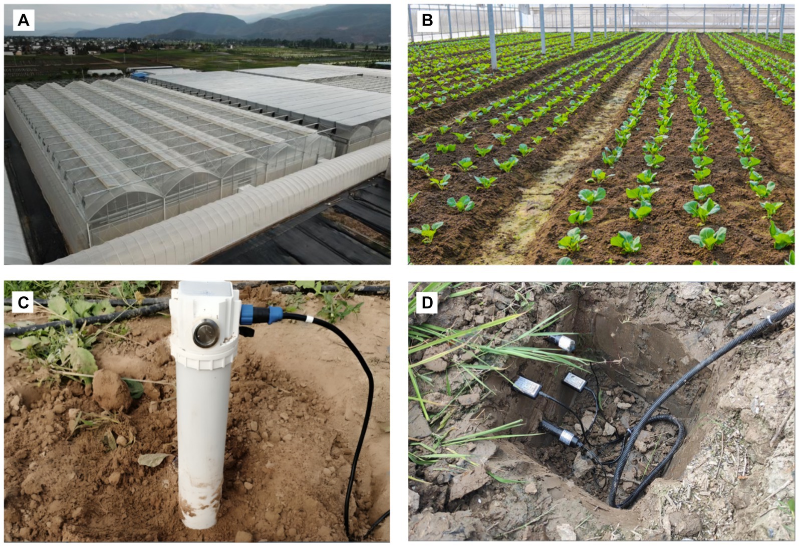
Figure 2. The komatsuna production environment and soil monitoring equipment. (A) The greenhouse vegetable production base; (B) The kumatsuna olantation area; (C) The vegetable soil detector; (D) The soil monitoring surface sensor.

2.2.2 Data acquisition and pre-processing

Figure 3 shows the soil parameter collection methods. The land type, land status, alkaline hydrolysis nitrogen, available phosphate, available potassium and other contents are measured. Each small plot is 60 ft. × 30 ft. through the layered grid sampling method (Sasikala and Ratha Jeyalakshmi, 2021). In each grid, the plum blossom sampling method is used for soil sampling (Mildenhall et al., 2019). The soil samples of 5 points are mixed and put into soil sampling bags for labeling. The mixed soil represents the soil fertility of the entire region.

Figure 3

Figure 3. The soil parameter collection methods. (A) The structure of the layered grid sampling method; (B) The plum blossom sampling method.

When the soil sample is obtained from the farm, it is air-dried, ground, sieved, and mixed to determine its content. The contents of alkaline hydrolysis nitrogen, available phosphate, available potassium are determined by the Kjeldahl method (Solangi et al., 2019), the molybdenum antimony anti-colorimetric method (Liu et al., 2022) and flame photometry method (Hemachandiran et al., 2023), which can obtain the soil nutrient data of the corresponding sampling points in each plot, so these data are sorted out. Table 1 shows the nutrient data of some soil samples from the experimental plot. It has six attributes for each sample: plot number, sampling soil depth, alkaline hydrolysis nitrogen, available phosphate, available potassium and other contents.

Table 1

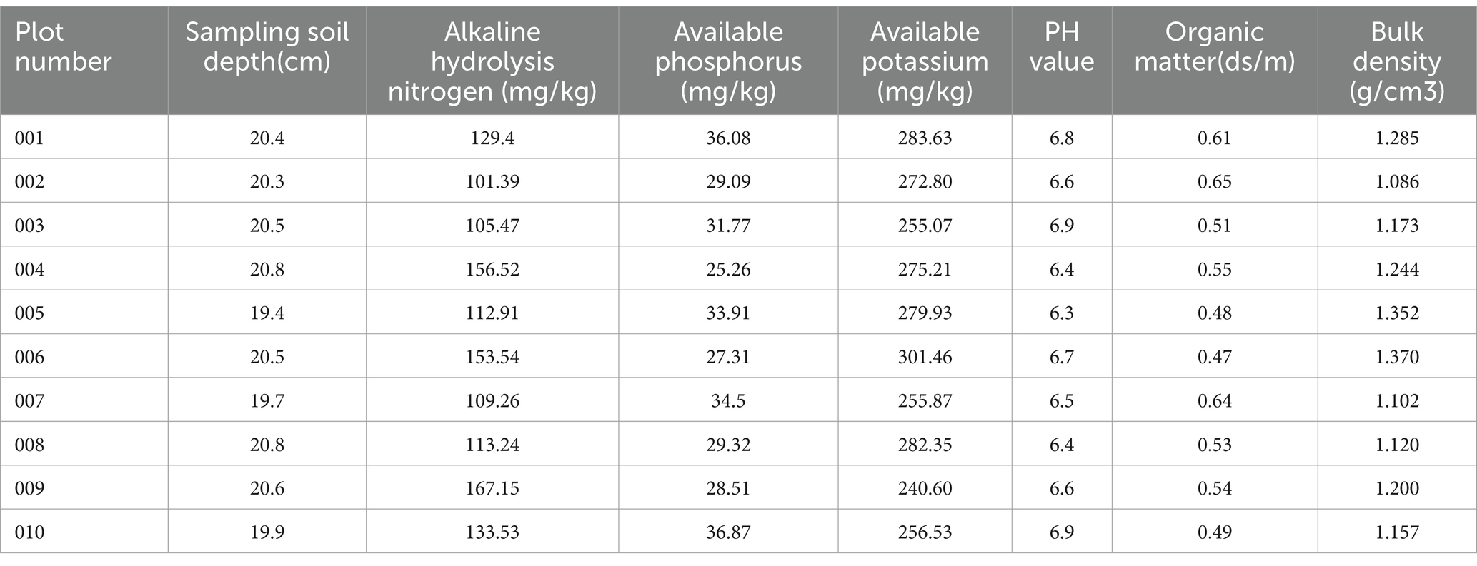
Table 1. The nutrient data of some soil samples from the experimental plot.

Due to the large differences in the attributes of soil data, larger inputs can suppress smaller inputs during the training process, which will not only slow down the training speed but also lead to the convergence failure (Roberts et al., 2022). In order to achieve better results, the difference of the data impact is eliminated, which ensured that the data variation is the same level. It also maintain the stability of the model and avoid the above errors. So the z-score normalization method is applied to preprocess the data before they are used for the model training (Ahmed et al., 2024). The z-score normalization subtracts the average value of the attribute from each attribute in each data object. The difference is divided by the variance of the attribute, as shown in Formula 12:

$\begin{array}{ll}\overline{s_{\tau }}=\frac{s_{\tau }-\sigma }{l_{\tau }}& (12)\end{array}$

In Formula 12, $s_{\tau }$ represents the $\tau -th$ standardized data attribute value, $\overline{s_{\tau }}$ represents the $\tau -th$ data attribute value to be standardized, $\sigma$ represents the mean value of the attribute, $l_{\tau }$ represents the variance of the attribute. Based on the results, the data standardized by this method conforms to standard the normal distribution. The mean value of standardized data is 0, and the variance is 1.

2.2.3 Model building

(1) Parameter setting

For the model training, 2000 sets of soil sample data are used, which has 1,600 sets for training and 400 for verification. According to the IM-BPNN model, the input and output layer unit numbers are set to 9 and 2. The Sigmoid function is taken as the activation function of the hidden layer neurons (Panda and Panda, 2020). The soil natural fertility parameters of the farmland in the experiment are alkaline hydrolysis nitrogen (128.241 mg/kg), available phosphorus (31.262 mg/kg), available potassium (270.345 mg/kg), organic matter (0.547ds/m), PH value (6.61) and bulk density (1.209 g/cm3), which are denoted by ${\mathrm{p}}_1$ , ${\mathrm{p}}_2$ , ${\mathrm{p}}_3$ , ${\mathrm{p}}_4$ , ${\mathrm{p}}_5$ , ${\mathrm{p}}_6$ , so the unit komatsuna yield is represented by ${\mathrm{p}}_7$ .

(2) Proportion determination

In order to extract the proportion of various element parameters in the soil, the relationship of the fertility parameters is identified by the neural network weight analysis function (Lou et al., 2022). According to the relationship between the various elements in the soil fertility indexes, the analysis weight of each index is determined. The BPNN is extensively trained using the BPNN algorithm’s learning rules and the TensorFlow Linspace function multiple times. The training is terminated when the training results meet the error accuracy requirements. The analytical weights for soil fertility indicators in the IM-BPNN algorithm are obtained.

Table 2 shows the connection weight fertility matrix of the IM-BPNN algorithm. The analysis weight order of the BPNN algorithm is available phosphorus > available potassium > alkaline hydrolysis nitrogen > organic matter > PH > bulk density. The weight variable of each element node is determined through multiple comparisons and analyses of the fertility weights of soil element information in the BPNN algorithm. The weight is effective, and the entire network training process is hardly affected except by the model itself. Therefore, the weighted results of IM-BPNN algorithm can maintain a high accuracy.

Table 2

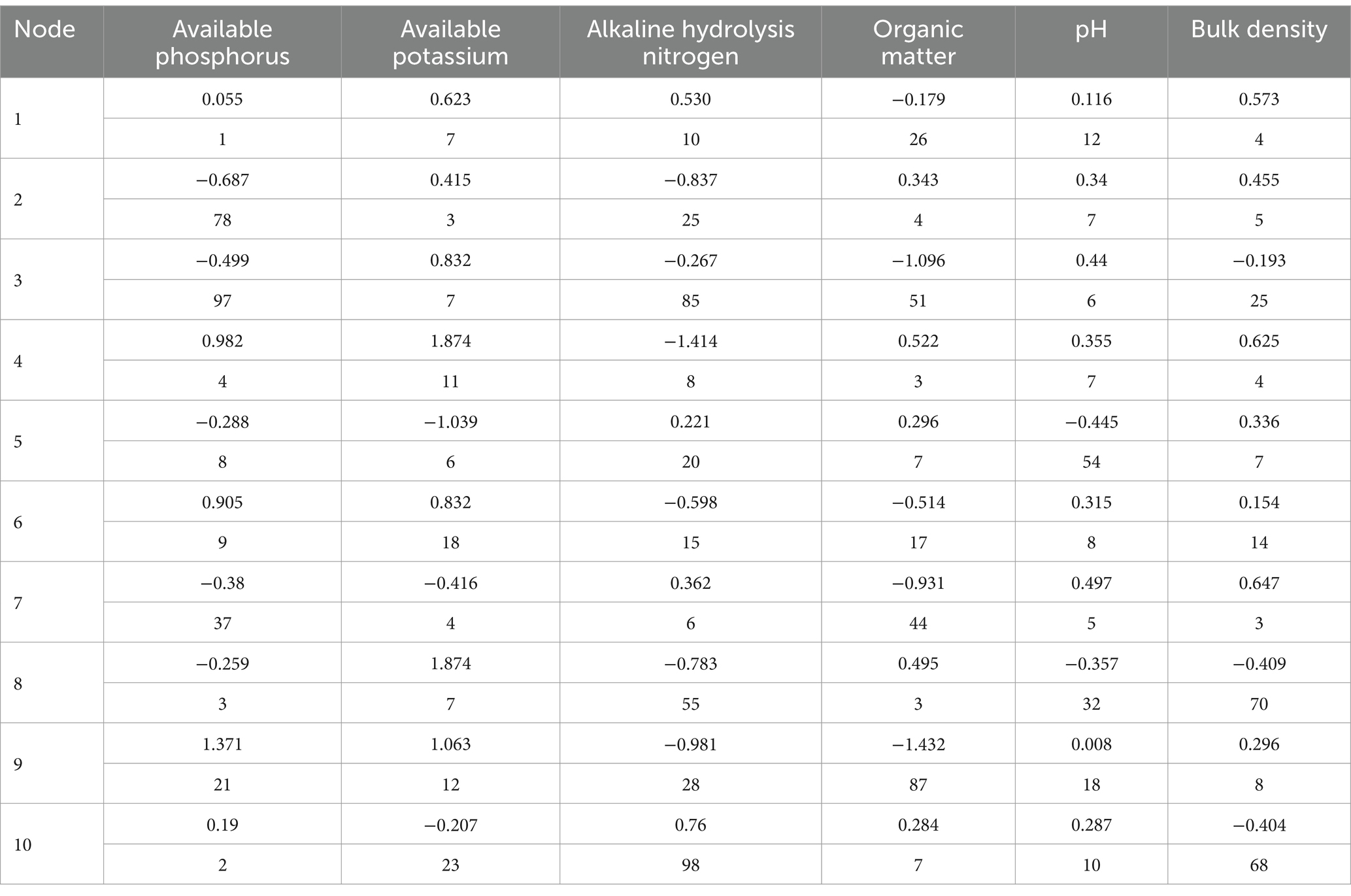
Table 2. The neural network soil fertility matrix with connection weights.

(3) Determination of network hierarchy

The optimal number of hidden layers and nodes in the neural network are determined in this study. Firstly, the number of hidden nodes in the BPNN algorithm is optimized by the dual particle swarm algorithm and four layers of a nonlinear network with Nihl neurons (Yu et al., 2022). The training accuracy of the network model is improved, and the network error is reduced by increasing the number of hidden layers or nodes in the hidden layers. Finally, after a lot of training on different neural network structures, it is found that when there is an hidden layer and 18–28 units in every layer. The training effect is best, so the magnitude of the training error is not large, which can keep stable.

3 Results and discussion

3.1 Experimental result

To prove the model’s accuracy, the amount of fertilizer applied to the original data is calculated by the unimproved BPNN algorithm, the NBTY (nutrient balance target yield) algorithm and the IM-BPNN algorithm. In order to estimate the fertilization amount for the target yield, the NBTY algorithm takes the target yield of crops, the difference between the amount of soil nutrients and supplied soil fertilizer as factors, so the balance of nutrients can be reached. According to the mathematical model of standard fertilization, the analysis result of sample data is as follows: 261 milligrams of available potassium, 37 milligrams of available phosphate, 280 milligrams of alkaline hydrolysis nitrogen are absorbed by every kilogram of Komatsuna soil [30], which is the fertilizer utilization rates of K, P, and N being 38, 27 and 56%.

(1) Available potassium fertilization prediction

Figure 4A shows the three algorithms for Potassium fertilizer prediction. The potassium amounts given by the NBTY and BPNN algorithm are in the range of 0–300 mg/kg. The amounts of fertilization less than 50 mg/kg are 5.70 and 2.45%; The amounts of fertilization in the range of 100–250 mg/kg (the reasonable potassium range) are 73.65 and 86.60%. Compared with the NBTY and BPNN algorithm, the potassium amounts suggested by the IM-BPNN algorithm are all in 100–250 mg/kg, and the prediction accuracy rate has increased by 35.78 and 15.47%. Meanwhile, 89.35% of the decision values are 100–200 mg/kg (the best potassium range), and the prediction accuracy rate has increased by 52.09 and 19.85%. Therefore, the fertilization model based on the IM-BPNN algorithms is more accurate and reasonable than another two algorithms.

Figure 4

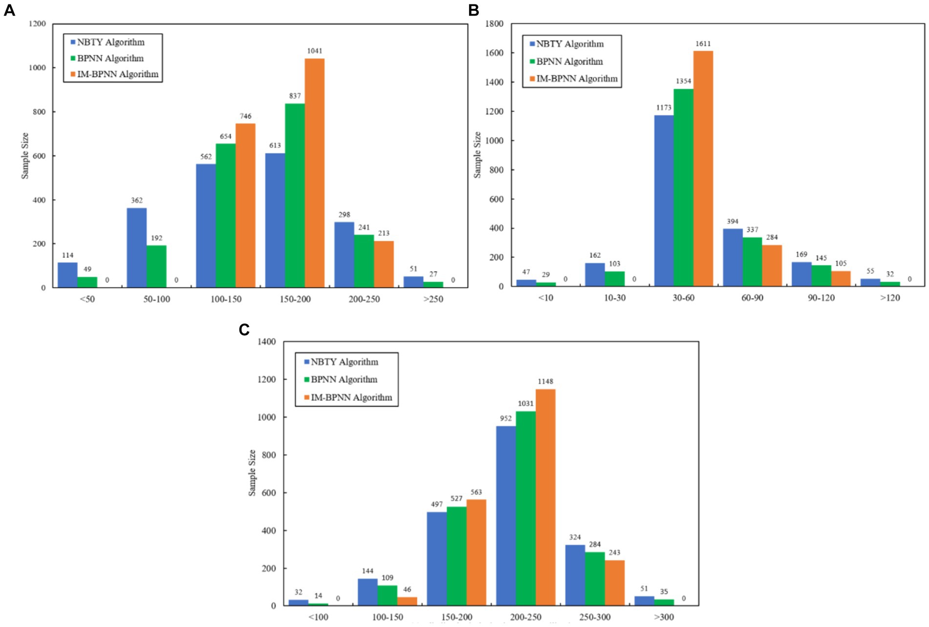
Figure 4. The fertilization prediction distribution of three algorithms. (A) Potassium fertilization range; (B) Available phosphate fertilization range; (C) Alkaline hydrolysis nitrogen fertilization range.

(2) Available phosphate fertilization prediction

Figure 4B shows the three algorithms for phosphate fertilizer prediction. Due to the large variation of soil available phosphate, it is difficult to calculate the correction coefficient of soil available phosphate. For the NBTY and BPNN algorithm, the suggested fertilization amounts in 30–90 mg/kg (the reasonable phosphate range) are 78.35 and 84.55%; the suggested fertilization amounts in 30–60 mg/kg (the best phosphate range) are 58.65 and 67.70%.Compared with the NBTY and BPNN algorithm, the phosphate amounts suggested by the IM-BPNN algorithm in the range of 30–90 mg/kg are 94.75%, which show that the prediction accuracy rate has increased by 20.93 and 12.06%. The decision values in the range of 100–200 mg/kg are 80.55%, which show that the prediction accuracy rate has increased by 37.34 and 18.98%. Therefore, the fertilization model based on the IM-BPNN algorithm is more accurate and reasonable than another two algorithms.

(3) Alkaline hydrolysis nitrogen fertilization prediction

Figure 4C shows the three algorithms for Nitrogen fertilizer prediction. For the NBTY and BPNN algorithm, the suggested amounts in 150–250 mg/kg (the reasonable nitrogen range) are 72.45 and 77.90%; the suggested amounts in 200–250 mg/kg (the best nitrogen range) are 47.60 and 51.55%, which is easy to make mistakes in decision-making. Compared with the NBTY and BPNN algorithm, the nitrogen amounts suggested by the IM-BPNN algorithm in the range of 150–250 mg/kg are 85.55%, which show that the prediction accuracy rate has increased by 18.08 and 9.82%. The suggested nitrogen amounts in 200–250 mg/kg are 80.55%, which show that the prediction accuracy rate has increased by 20.59 and 11.35%. Therefore, the IM-BPNN algorithm is more accurate and reasonable than another two algorithms.

3.2 Discussions

This study achieved remarkable results in experiments on greenhouse vegetables (komatsuna) in Qingyuan City, Guangdong, China. But in order to ensure the effectiveness and reliability of the IM-BPNN algorithm in wider applications, in subsequent research, it also need to collect data from Data for different geographical locations, different crops and different soil types. Through training on diverse data, the generalization ability of the model can be improved so that it can perform well in more scenarios. Furthermore, experiments are conducted under different environmental conditions and agricultural practices to verify the performance of the algorithm under different conditions, which improves the robustness and adaptability of the algorithm. It will also conduct research on more crops and analyze the applicability of the algorithm on different crops. By comparing the experimental results of different crops, the parameters can be optimized and its prediction capabilities on different crops can be enhanced. Through these measures, the IM-BPNN algorithm will be able to demonstrate its potential in a wider range of agricultural applications and provide reliable and efficient solutions for precision agriculture.

In addition, this study conducts research based on two assumptions: the IM-BPNN algorithm can predict the amount of fertilizer required for greenhouse vegetables more accurately than the BPNN and NBTY algorithms, and the introduction of the double particle swarm optimization algorithm can improve the accuracy and efficiency of the BPNN algorithm in fertilizer decision-making. And made corresponding research contributions in algorithm innovation and multi-variable comprehensive analysis. In terms of algorithm innovation, this study introduced the dual particle swarm algorithm to improve the BPNN algorithm. It has not been widely used in existing fertilization decision-making methods, filling the research gap in this field. The IM-BPNN algorithm combines the nonlinear fitting ability of BPNN and the global search ability of the dual particle swarm optimization algorithm to improve the convergence speed and prediction accuracy of the model. This innovation provides a new technical means for intelligent agricultural management. In the multi-variable comprehensive analysis, this study analyzed the relationship between multiple soil nutrient indicators (such as alkali-hydrolyzable nitrogen, available phosphorus, available potassium, etc.), determined the weight of each indicator’s impact on crop growth, and established a comprehensive Fertilization decision model. It can comprehensively consider multiple influencing factors to achieve more scientific fertilization decisions and improve crop yield and quality.

Although the IM-BPNN algorithm proposed in this study is better at predicting the amount of fertilizer required for these three nutrients in the future through the historical data of soil nutrients such as alkali-hydrolyzable nitrogen, available phosphorus and available potassium. However, factors that affect crop growth and nutrient requirements also include trace elements, soil pH, and other soil characteristics that have an impact on the overall nutrient requirements of crops, so subsequent research needs to explore the possibility of more factors affecting crop growth and nutrient requirements. Furthermore, real-time data collection and monitoring of crops are very necessary measures. Follow-up research will also need to integrate real-time data collection methods, such as sensors and Internet of Things (IoT) devices, to continuously monitor soil conditions and dynamic changes in the environment. Through the above measures, the samples for IM-BPNN algorithm training can be expanded to avoid problems such as the IM-BPNN algorithm falling into local optimal solutions when the amount of data is small, thereby improving the accuracy of algorithm prediction. The final step is to apply the algorithm to the corresponding user interface or mobile application, allowing farmers to easily enter data and obtain actionable recommendations in an easy-to-understand format, which facilitates the application of the algorithm in actual scenarios. Figure 5 shows the precision fertilization monitoring application graphical user interface.

Figure 5

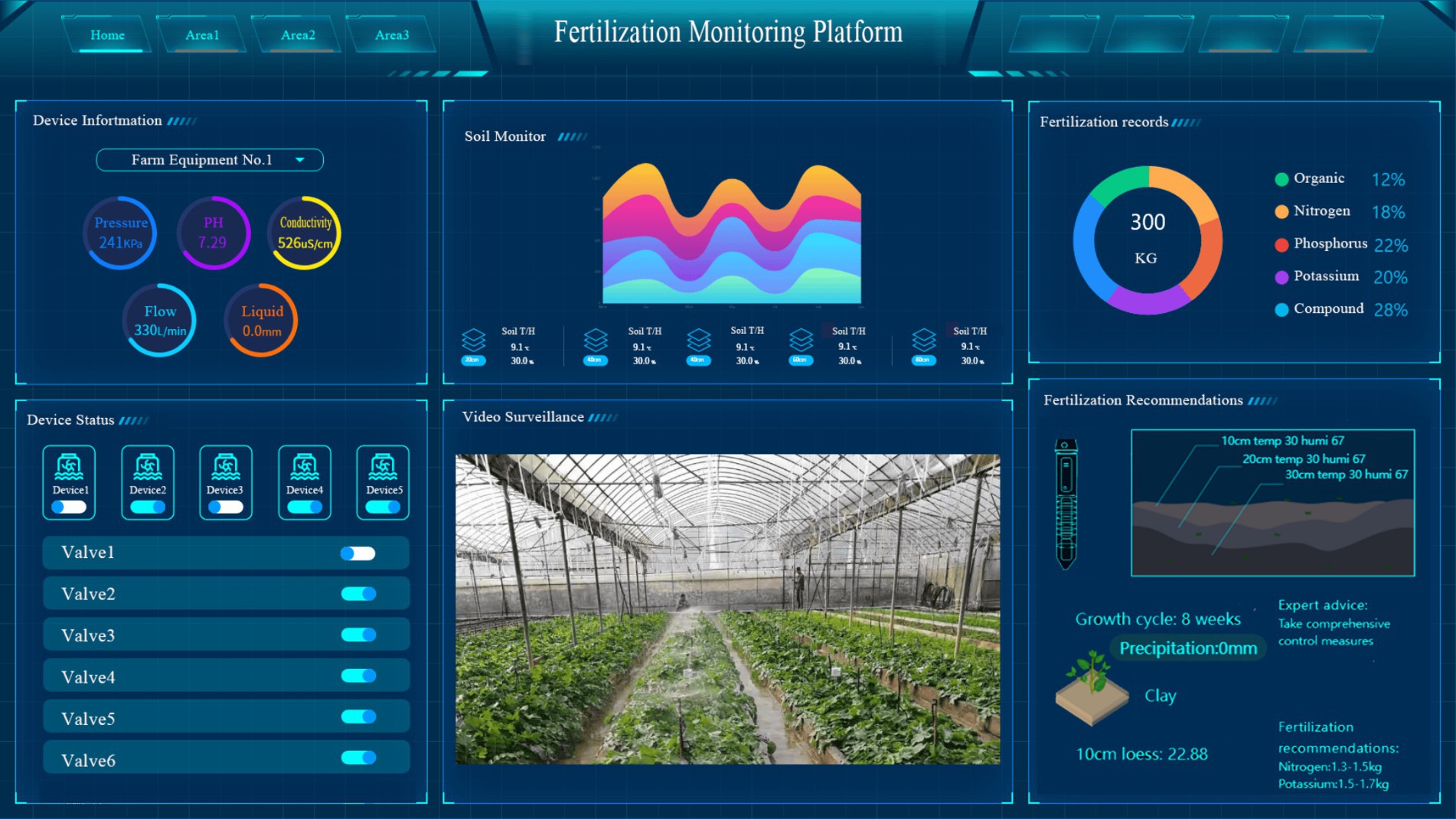
Figure 5. The precision fertilization monitoring application graphical user interface.

4 Conclusion

In this study, a greenhouse vegetable precision fertilization method based on the IM-BPNN algorithm is designed. It introduces the dual particle swarm optimization algorithm to improve the accuracy of the BPNN algorithm, which builds the IM-BPNN algorithm. Compares with the NBTY and BPNN algorithm, the predictive potassium amounts are all in 100–250 mg/kg, and the predictive accuracy rate improves 35.78 and 15.47%. The predictive phosphate amounts in the range of 30–90 mg/kg are 94.75%, and the predictive accuracy rate has increased 20.93 and 12.06%. The predictive amounts suggested in the range of 150–250 mg/kg are 85.55%, and the predictive accuracy rate has increased 18.08 and 9.82%.It shows that the decision-making accuracy of is the IM-BPNN algorithm higher than the another two algorithms. Through the method proposed in this study, it can more accurately determine the amount of fertilizer required by vegetables, avoid over-application, and reduce negative impacts on the environment, which improves the fertilizer utilization efficiency and agricultural environmental protection. It also helps farmers reduce fertilizer waste, lowers production costs and improves the economic viability of agriculture.

Data availability statement

The original contributions presented in the study are included in the article/supplementary material, further inquiries can be directed to the corresponding author.

Ethics statement

For the field survey involving human participants, the study followed the guidelines of the 1964 Helsinki Declaration and its amendments.

Author contributions

RT: Conceptualization, Methodology, Software, Validation, Formal analysis, Investigation, Data curation, Writing – original draft, Writing – review & editing, Visualization. WS: Conceptualization, Methodology, Validation, Formal analysis, Writing – review & editing. NA: Resources, Project administration, Writing – review & editing. MT: Writing – review & editing, Supervision, Resources. XY: Software, Data curation, Visualization, Writing – review & editing.

Funding

The author(s) declare that no financial support was received for the research, authorship, and/or publication of this article.

Conflict of interest

The authors declare that the research was conducted in the absence of any commercial or financial relationships that could be construed as a potential conflict of interest.

Publisher’s note

All claims expressed in this article are solely those of the authors and do not necessarily represent those of their affiliated organizations, or those of the publisher, the editors and the reviewers. Any product that may be evaluated in this article, or claim that may be made by its manufacturer, is not guaranteed or endorsed by the publisher.

References

Ahmed, H. M., Elsheweikh, D. L., and Shaban, S. A. (2024). Security system based on hand geometry and palmprint for user authentication in E-correction system. Int. J. Inf. Technol. 16, 1783–1799.

Google Scholar

Ashraf, H., Sultan, M., Shamshiri, R. R., Abbas, F., Farooq, M., Sajjad, U., et al. (2021). Dynamic evaluation of desiccant dehumidification evaporative cooling options for greenhouse air-conditioning application in Multan (Pakistan). Energies 14:1097. doi: 10.3390/en14041097

Crossref Full Text | Google Scholar

Brunetto, G., Stefanello, L. O., Kulmann, M. S. D. S., Tassinari, A., Souza, R. O. S. D., Rozane, D. E., et al. (2022). Prediction of nitrogen dosage in ‘Alicante bouschet’vineyards with machine learning models. Plan. Theory 11:2419. doi: 10.3390/plants11182419

PubMed Abstract | Crossref Full Text | Google Scholar

Chen, N., Xiong, C., Du, W., Wang, C., Lin, X., and Chen, Z. (2019). An improved genetic algorithm coupling a back-propagation neural network model (IGA-BPNN) for water-level predictions. WaterSA 11:1795. doi: 10.3390/w11091795

Crossref Full Text | Google Scholar

Coulibali, Z., Cambouris, A. N., and Parent, S. É. (2020). Site-specific machine learning predictive fertilization models for potato crops in eastern Canada. PloS one 15:e0230888. doi: 10.1371/journal.pone.0230888

PubMed Abstract | Crossref Full Text | Google Scholar

Dong, Y., Fu, Z., Peng, Y., Zheng, Y., Yan, H., and Li, X. (2020). Precision fertilization method of field crops based on the wavelet-BP neural network in China. J. Clean. Prod. 246:118735. doi: 10.1016/j.jclepro.2019.118735

Crossref Full Text | Google Scholar

Gunawan, A., Thamrin, S., Kuntjoro, Y. D., and Idris, A. M. (2022). Backpropagation neural network (BPNN) algorithm for predicting wind speed patterns in East Nusa Tenggara. Trends in Renewable Energy 8, 107–118. doi: 10.17737/tre.2022.8.2.00143

Crossref Full Text | Google Scholar

Hemachandiran, S., Siddharth, R., and Aghila, G. (2023). A digital image colorimetry approach for identifying fuel types in downstream petroleum sector. Int. J. Inf. Technol. 15, 1443–1452. doi: 10.1007/s41870-023-01206-w

Crossref Full Text | Google Scholar

Jain, A., Pal Nandi, B., Gupta, C., and Tayal, D. K. (2020). Senti-NSetPSO: large-sized document-level sentiment analysis using Neutrosophic set and particle swarm optimization. Soft. Comput. 24, 3–15. doi: 10.1007/s00500-019-04209-7

Crossref Full Text | Google Scholar

Jin, X., Zhao, K., Ji, J., Qiu, Z., He, Z., and Ma, H. (2020). Design and experiment of intelligent monitoring system for vegetable fertilizing and sowing. J. Supercomput. 76, 3338–3354. doi: 10.1007/s11227-018-2576-2

Crossref Full Text | Google Scholar

Junfeng, Z. H. A. N. G., Jialin, K. U. A. I., Xiaowei, W. A. N. G., Yuxin, Z. H. A. N. G., and Yanxia, M. A. (2022). Effects of combined application of nitrogen, phosphorus and potassium on yield and quality of tomato cultured with organic substrate in greenhouse. J. Northwest A & F University-Natural Sci. Edition 50.

Google Scholar

Liu, C., Zhuang, J., Wang, J., Fan, G., Feng, M., and Zhang, S. (2022). Soil bacterial communities of three types of plants from ecological restoration areas and plant-growth promotional benefits of Microbacterium invictum (strain X-18). Front. Microbiol. 13:926037. doi: 10.3389/fmicb.2022.926037

PubMed Abstract | Crossref Full Text | Google Scholar

Lou, S., Hu, R. Q., Liu, Y., Zhang, W. F., and Yang, S. Q. (2022). The formulation of irrigation and nitrogen application strategies under multi-dimensional soil fertility targets based on preference neural network. Sci. Rep. 12:20918. doi: 10.1038/s41598-022-25133-1

PubMed Abstract | Crossref Full Text | Google Scholar

Mildenhall, B., Srinivasan, P. P., Ortiz-Cayon, R., Kalantari, N. K., Ramamoorthi, R., Ng, R., et al. (2019). Local light field fusion: practical view synthesis with prescriptive sampling guidelines. ACM Transac. Graphics (TOG) 38, 1–14. doi: 10.1145/3306346.3322980

Crossref Full Text | Google Scholar

Panda, S., and Panda, G. (2020). Fast and improved backpropagation learning of multi-layer artificial neural network using adaptive activation function. Expert. Syst. 37:e12555. doi: 10.1111/exsy.12555

Crossref Full Text | Google Scholar

Qiuying, Ma . (2017). Cost-benefit analysis of the main utilization methods of corn straw in Northeast China (Doctoral dissertation, Beijing: Chinese Academy of Agricultural Sciences).

Google Scholar

Recena, R., Fernández-Cabanás, V. M., and Delgado, A. (2019). Soil fertility assessment by Vis-NIR spectroscopy: predicting soil functioning rather than availability indices. Geoderma 337, 368–374. doi: 10.1016/j.geoderma.2018.09.049

Crossref Full Text | Google Scholar

Rezvani, S. M. E. D., Shamshiri, R. R., Hameed, I. A., Abyane, H. Z., Godarzi, M., Momeni, D., et al. (2021). Greenhouse crop simulation models and microclimate control systems, a review. Next-Generation Greenhouses for Food Security. doi: 10.5772/intechopen.97361

Crossref Full Text | Google Scholar

Roberts, T. M., Colwell, I., Chew, C., Lowe, S., and Shah, R. (2022). A deep-learning approach to soil moisture estimation with GNSS-R. Remote Sens. 14:3299. doi: 10.3390/rs14143299

Crossref Full Text | Google Scholar

Sasikala, S., and Ratha Jeyalakshmi, T. (2021). GSCNN: a composition of CNN and Gibb sampling computational strategy for predicting promoter in bacterial genomes. Int. J. Inf. Technol. 13, 493–499. doi: 10.1007/s41870-020-00565-y

Crossref Full Text | Google Scholar

Shamshiri, R. R., Bojic, I., van Henten, E., Balasundram, S. K., Dworak, V., Sultan, M., et al. (2020). Model-based evaluation of greenhouse microclimate using IoT-sensor data fusion for energy efficient crop production. J. Clean. Prod. 263:121303. doi: 10.1016/j.jclepro.2020.121303

Crossref Full Text | Google Scholar

Shamshiri, R. R., Hameed, I. A., Thorp, K. R., Balasundram, S. K., Shafian, S., Fatemieh, M., et al. (2021). Greenhouse automation using wireless sensors and IoT instruments integrated with artificial intelligence. Next-generation greenhouses for food security. doi: 10.5772/intechopen.97714

Crossref Full Text | Google Scholar

Shamshiri, R, Kalantari, F., Ting, K. C., Thorp, K. R., Hameed, I. A., and Weltzien, C. (2018). Advances in greenhouse automation and controlled environment agriculture: A transition to plant factories and urban agriculture. Int. J. Agric. Biol. Eng. 11, 1–22.

Google Scholar

Sharma, A., Vora, D., Shaw, K., and Patil, S. (2023). Sentiment analysis-based recommendation system for agricultural products. Int. J. Inf. Technol. 16, 761–778.

Google Scholar

Solangi, F., Bai, J., Gao, S., Yang, L., Zhou, G., and Cao, W. (2019). Improved accumulation capabilities of phosphorus and potassium in green manures and its relationship with soil properties and enzymatic activities. Agronomy 9:708. doi: 10.3390/agronomy9110708

Crossref Full Text | Google Scholar

Swaminathan, B., Palani, S., and Vairavasundaram, S. (2023). Feature fusion based deep neural collaborative filtering model for fertilizer prediction. Expert Syst. Appl. 216:119441. doi: 10.1016/j.eswa.2022.119441

Crossref Full Text | Google Scholar

Youlu, B. (2018). Current status and prospect of research on high-efficiency fertilization technology. Chinese. Agric. Sci. 51:21.

Google Scholar

Yu, F., Bai, J., Jin, Z., Zhang, H., Guo, Z., and Chen, C. (2022). Research on precise fertilization method of rice tillering stage based on UAV hyperspectral remote sensing prescription map. Agronomy 12:2893. doi: 10.3390/agronomy12112893

Crossref Full Text | Google Scholar

Zhang, J., He, P., Ding, W., Xu, X., Ullah, S., Abbas, T., et al. (2019). Estimating nutrient uptake requirements for radish in China based on QUEFTS model. Sci. Rep. 9:11663. doi: 10.1038/s41598-019-48149-6

PubMed Abstract | Crossref Full Text | Google Scholar