Effects of agricultural subsidies on farm household decisions: a separable household model approach

Introduction: This study employs a separable household model to estimate the effect of agricultural subsidies on production and consumption decisions taken by farm households. The study used data from a household survey using a pre-tested schedule to develop and calibrate an agricultural household model.

Method: First, we calculated a price index for the model. The index was higher for non-agricultural commodity groups in all the categories of farm households. Expenditure on non-agricultural commodity groups was more than agricultural commodity groups.

Result and Discussion: Results indicated that for the agricultural commodity group, the estimated coefficients of linear expenditure system (LES) model were positive and less than one for all farm household categories except for the wage-price coefficient which was found to be negative. The estimates of profit function in the study area depict that the variable inputs were negatively related to the profit function and the fixed inputs were positively related to profit. Our study highlights a few crucial points – First, the removal of subsidies will decrease the demand for electricity, concentrate and irrigation by 80, 73 and 70 %, respectively. Second, removing subsidies will not only affect the demand for inputs but will also lead to a decline in the consumption demand for both agricultural and non-agricultural commodities. Third, this effect was found to be more prominent in the small and medium categories of farm households.

1 Introduction

The farmer-centric approach to agricultural policies was adopted in the 1960s when India transformed its agriculture sector during the Green Revolution. These policies required increased utilization of high-yielding seed varieties, fertilizers, and irrigation. However, a significant portion of the farming community, consisting of small and marginal farmers, found these inputs unaffordable. As a result, the government initiated subsidies on various inputs, including fertilizers, electricity, and seeds. This made agricultural inputs available at prices lower than the free-market rates, incentivizing increased input usage and subsequent production by farm households. Micro-level analyses on subsidies also indicated that the availability of expensive inputs at reduced prices led to the adoption of newer technologies (Narayanamoorthy, 1997). In fact, several studies demonstrated that lower input costs and the adoption of newer technologies resulted in increased incomes for farmers (Pandey and Khanna, 1980; Garg and Dhaliwal, 1982; Yadav et al., 1982). The lower input cost leads to an increase in the real income of the farmers, which gives the incentive to divert their additional income toward other income-generational activities. The adoption of newer technology leads to a shift in the frontier; thus, higher productivity and incorporation of diverse product range by farmers (Ruzzante et al., 2021).

However, there were other consequences as well, such as the failure to reach the intended targets in the case of fertilizer subsidies (Gulati, 1990) and a change in cropping patterns. Researchers have argued that subsidies have become unsustainable due to their high costs to the government (25% of government spending) (Jones, 2013). It has been suggested that without financial support, there will be an increase in the income gap between rural and urban areas, leading to depeasantization (Henningsen et al., 2009). Moreover, the long-term costs of subsidy programs outweigh the benefits and have negative effects on sustainable development (Fan et al., 2009; Jayne and Rashid, 2013). These factors have necessitated a re-examination of subsidies as a policy instrument for farmers' welfare. A research study in sub-Saharan Africa depicts that the subsidy on legume seeds increased land allocation and led to an increase in the area planted for legumes (Khonje et al., 2021). The analysis of farm households is of great importance, as one-fourth of the world's population is engaged in farming (Ellis, 1988). The success of agricultural policies implemented by governments depends on household characteristics and their decision-making processes. A typical farm household faces three intertwined decisions: production, consumption, and farm labor. To study the intricacies of these decisions, a separable household model was employed in this study. In India, a significant proportion of farmers are subsistence farmers, meaning that their farms are semi-commercialized, with some produce intended for the market and some for personal consumption. In agricultural production, essential resources, such as fertilizers, seeds, and hired labors, are procured through the market transaction, while other inputs, such as family labor, are used implicitly. Therefore, any policy change related to agricultural activities have an impact not only on production but also on input demand and labor supply.

Earlier studies have primarily focused on the effects of subsidies on farm income, overlooking the overall impact (Pandey and Khanna, 1980; Mishra and Goodwin, 1997; Acharya, 2000). However, an agricultural household is involved in both production and consumption activities, and policies that affect the prices of factors that are both produced and consumed have complex implications for production and the welfare of agricultural households (Sadoulet and de Janvry, 1995). Several econometric studies have been conducted in other countries to analyze the effects of specific subsidies on various aspects such as time allocation (Mishra and Goodwin, 1997; El-Osta et al., 2004; Ahearn et al., 2006; Dewbre and Mishra, 2007), productivity (Bezlepkina and Oude Lansink, 2006; Guan and Oude Lansink, 2006; Skuras et al., 2006; McCloud and Kumbhakar, 2008; Rizov et al., 2013), efficiency (Piesse and Thirtle, 2000; Giannakas et al., 2001; Karagiannis and Sarris, 2005; Hadley, 2006; Kleinhanß et al., 2007), and transfer efficiency (Bergström, 2000; Dewbre and Mishra, 2007).

In this study, we apply a separable household model to estimate the effect of government agricultural subsidies on farm households. The agricultural household model allows us to analyze the consequences of policy in three sub-dimensions. First, we examine the consumption preferences of sample households across different categories of farm households under budget constraints. Second, we analyze the effect of subsidy removal on the demand for inputs and labor across different categories of farm households. Finally, we investigate the impact of subsidy removal on the marketed surplus of farm households.

To achieve these objectives, Section 2 presents the theoretical model, analytical tools, and the methodology employed. Following the description of our approach, Section 3 focuses on the sample design, data collection, and descriptive statistics. Econometric results and analysis are presented in Section 4, and concluding comments are provided in Section 5.

2 Methodology and theoretical framework

Farmers receive subsidies for various inputs and activities related to growing crops, such as the purchase of seeds, fertilizers, electricity, farm implements, loans/credit, land leveling, reclamation, plant protection, as well as extension and training. Similarly, in livestock activities, subsidies are provided for the purchase of animals, feed, loans, insurance, and veterinary and health services. The calculation of subsidies at the household level is done using two approaches. First, subsidies are targeted at specific categories of farm households. Second, pro rata subsidies are estimated by multiplying the quantity of input used by the subsidy per unit. The amount of subsidy received by each household varies depending on the programs and schemes availed by the farmers and the amount of subsidized input used.

The subsidy for seeds, fertilizers, and electricity is estimated on a pro-rata basis, while the subsidy for loans, purchase of implements/animals, insurance, extension, and training is based on the items purchased under specific schemes meant for farmer categories, such as small and marginal farmers, SC & ST, BPL, or Antodaya. The subsidies provided by the government to different categories of farmers determine the effective prices paid by the farmers for different inputs and services. The effective price paid is obtained by subtracting the subsidy per unit from the market price per unit. These effective prices are used in the separable household model described below.

For the analysis, the Separable Household Model is used to determine the effect of subsidies on production, consumption, and labor supply. The farm household is assumed to maximize utility while considering factors such as time, budget/income, technology, and resources. Our model takes into account the linkages of farm subsidies, the endogeneity of input use, and farm production. In this model, as the prices are exogenous to the household and there are no transaction costs, it is irrelevant whether the household consumes its own produce or sells it off. Thus, there is a condition of separability where prices are exogenous, which is why this model is used.

Household models are designed to capture interactions so that policy interventions can be empirically estimated. The effects of policy interventions, such as subsidies distributed to farmers, impact not only the production decisions but also the consumption and labor supply of farm households. Therefore, household models are applied to analyze and understand the consequences of policy implications across these three dimensions. In the separable household model, consumption preferences depend on production through the common term known as full income. Full income includes not only the household's profit but also the imputed value of labor used for production. This is depicted in Figure 1, which illustrates the main biophysical and socioeconomic components of the model and their linkages. Profit serves as a key factor connecting both production and consumption activities/decisions.

FIGURE 1

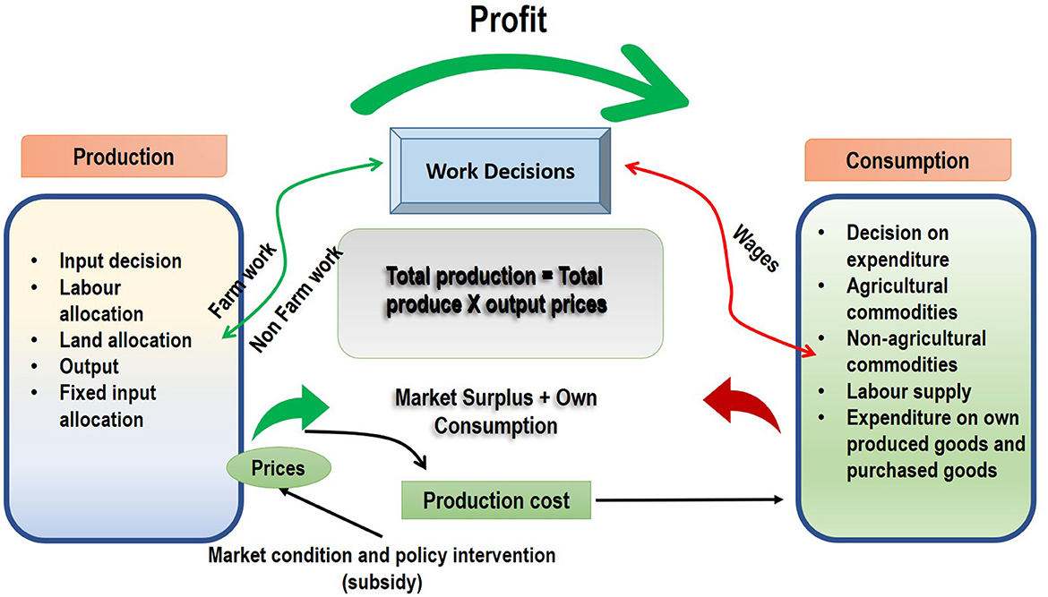
Figure 1. Structure of separable household model.

For the analysis, the production and consumption decisions in the household model were estimated as discussed below:

2.1 Production decisions

The production decisions depict how households respond to changes in product and factor prices. The production function of a farm illustrates the relationship between output and variable inputs used, such as fertilizers and seeds, as well as the fixed factors, such as land and capital. By utilizing duality, production relationships can be better understood by estimating the profit function, where normalized profit becomes a function of the relative prices of inputs and the value of fixed factors. The use of the profit function to estimate the production relationship has the additional advantage of providing an enriched specification and deriving input demand functions through the direct application of Hottelings-Shephard's Lemmas. The normalized profit function gives rise to corresponding factor demand and output supply equations.

In the present study, a Cobb-Douglas type of normalized restricted profit function was employed, as shown below:

$\begin{array}{ll}ln({\pi }^{{}^{*}})={\beta }_0+{\displaystyle \sum _j}{\beta }_{j}ln\left(\frac{p_j}{p_a}\right)+{\displaystyle \sum _k}{\gamma }_{k}ln{z}_k& (1)\end{array}$

where the normalized profit function π^* is the ratio of profit to price of output ($\frac{\pi }{p_a}$). The p_j is the effective prices of various variable inputs and z_k is the value of fixed factors. The variable inputs considered in the function were labor, animal labor, machine labor, seed, fertilizer, electricity, feed, and fodder along with fixed inputs such as capital and land. The equation is homogeneous of degree one under restriction:

$\begin{array}{ll}{\displaystyle \sum _k}{\gamma }_k=1& (2)\end{array}$

Output supply q and input demand x_i function can be derived from the profit function. Output supply function was obtained by differentiating the profit function with respect to the price of a product. The input demand was obtained by taking a negative derivative of the normalized profit function with respect to the respective input price. The equations for the same is given as follows:

$\begin{array}{ll}q=\frac{\partial \pi }{\partial p_j}=(1+{\beta }_a)\frac{\pi }{p_a}& (3)\end{array}$

And

$\begin{array}{ll}{x}_i=-\frac{\partial \pi }{\partial p_j}=-{\beta }_j\frac{\pi }{p_j}& (4)\end{array}$

The profit obtained from the profit function was then used to calculate y^*, which acts as a hinge between production and consumption activities/decisions of a household as shown in the model above.

2.2 Consumption decisions

In a closed market, a farm household typically consumes what it produces and relies on its own labor. In this situation, consumption and labor decisions depend on the household's production and income. The literature offers two approaches for estimating demand: a single equation demand function, which pragmatically considers the observed behavior without explicitly incorporating economic theory, and a complete demand system of equations, which accounts for the mutual interdependence of a large number of commodities in the consumer's budget allocation and captures the consequences of simultaneous changes in variables (Subramanian et al., 2019). The single demand function may not fully satisfy the basic requirements of demand theory; therefore, complete demand systems are applied to estimate consumer preferences, taking into account the mutual interdependence of a large number of commodities subject to budgetary constraints.

The demand for different commodities in an agricultural rural household is further aggregated into three commodity groups (indexed by i = 1 to 3): demand for agricultural goods, demand for non-agricultural goods, and demand for home time. Here, we focus on explaining the demand for home time, which represents the time required for leisure and fulfilling personal and family needs. Consumption decisions involve a trade-off between allocating time for home-related activities and consuming goods that require more income and, consequently, more work. As a result, the demand for home time will decrease. To estimate the demand functions for agriculture, non-agriculture, and home time, the linear expenditure system (LES) was applied. The LES, developed by Stone (1954), is derived from the Stone–Geary utility function, which takes the following form:

$\begin{array}{ll}u={\displaystyle \prod _{i=1}^n{(q_i-c_i)}^{b_i}}\text{ such that }\{\begin{array}{c}\text{0}<{\text{b}}_{\text{i}}<\text{1}\\ {\displaystyle \sum _{\text{i}}{\text{b}}_{\text{i}}}\text{=1}\\ ({\text{q}}_{\text{i}}-\text{ ci})>\text{1}\end{array}& (5)\end{array}$

The c_i is the minimum subsistence consumption of i^th commodity or “committed” quantities below which consumption cannot fall. The q_i is the actual quantity of i^th commodity consumed and b_i is the marginal budget share, which tell how expenditure on each commodity changes as income changes. The demand functions derived from maximization of this utility function under a budget constraint constitute (y = ∑p_iq_i), when written in logarithmic form is known as a linear logarithmic expenditure system of the following type:

$\begin{array}{ll}{p}_i{c}_i=y^{{}^{*}}({\alpha }_{i0}+{\displaystyle \sum _k}{\alpha }_{ik}ln{p}_k+{\alpha }_{id}ln{A}_d)& (6)\end{array}$

Where y^* is the full income of the household, which is comprised of profit, total time endowment, and transfer payments as shown below:

$\begin{array}{ll}{y}^{{}^{*}}=\pi +p_{l}E{A}_w+S& (7)\end{array}$

The other variables in Equation 3 are p_l the wage rate, A_w the number of workers in a household, E the total time endowment available per worker, and S net transfers (positive or negative).

In equation, p_k is the prices of the different goods (agricultural commodity, non-agricultural commodity, and home time) and A_d is the number of members in the household. To run the equation, shares of expenditure on the i^th group of each commodity (p_iq_i/y^*) and price indices were formed for different commodity groups. Thus, the dependent variables used in demand function were share of expenditure on each commodity group from total expenditure of household, price index of each commodity group, and number of dependents as independent variables. The system of equations was estimated subject to restrictions on its parameters as follows:

$\begin{array}{ll}{\displaystyle \sum _i}{\alpha }_{i0}=1,{\displaystyle \sum _i}{\alpha }_{ik}=0and{\displaystyle \sum _i}{\alpha }_{ik}={\displaystyle \sum _i}{\alpha }_{id}=0& (8)\end{array}$

In the linear logarithmic expenditure system, a set of simultaneous equations exists that are highly interrelated. To obtain more unbiased estimates of parameters compared to ordinary least squares (OLS) estimates, Zellner (1962) method for iterative seemingly unrelated regression (SURE) technique was employed to estimate the model. This technique is used due to the singularity of the covariance matrix among residuals and the satisfaction of the budget constraint. Out of the three demand equations, the parameters of two equations were estimated using SURE, while the parameters of the remaining equation were estimated using an adding-up restriction.

In our analysis, the demand equation for home time was estimated using the aforementioned procedure. The other two equations were as follows:

$\begin{array}{l}{W}_{ag}=c(1)+c(2)*ln(p_a)+c{(3)}^{*}ln(p_{na})\hfill \\ +{(0-(c(2)+c(3)))}^{*}ln(ht)+c{(4)}^{*}ln(ad)\hfill \\ W_{nag}=c(5)+c{(3)}^{*}ln(p_a)+c{(6)}^{*}ln(p_{na})\hfill \\ +{(0-(c(3)+c(6)))}^{*}ln(ht)\hfill \end{array}$

Where “W_ag” denotes the share of the agricultural group of commodities in total household expenditure; “W_nag” denotes the share of the non-agricultural group of commodities in total household expenditure. The p_a and p_na denote the consumer price index of agriculture and non-agriculture commodities group of commodities, respectively. The “ht” denotes the price/wage index for home time and “ad” denotes the number of members/dependents in the household.

3 Survey design and data

To apply the HH model, household-level primary data were collected from three states. The analysis was conducted across household categories. The following section delineates the basic sampling design used to select households for data collection.

3.1 Sampling design

A multistage simple random sampling technique was utilized to select farm households across three states. In the first stage, all states in India were divided into three categories: high, medium, and low, based on the Agriculture Development Index (ADI) (refer to the Appendix for details). Using the cumulative square root frequency method, the states were categorized as low (ADI <0.3886), medium (ADI ranging from 0.3886 to 0.5993), and high (ADI > 0.5993). One state from each category was then randomly selected. Thus, Haryana was selected as the high agriculturally developed state, Rajasthan as the medium developed state, and Odisha as the low developed state, with ADI values of 0.6699, 0.4373, and 0.1778, respectively.

In the second stage of sampling, one district was purposefully selected from each state based on the criteria of satisfying the average conditions of the state in terms of per capita income and agricultural productivity. As a result, Jind, Udaipur, and Sundargarh districts were selected from Haryana, Rajasthan, and Odisha, respectively. In the next stage, two blocks were randomly chosen from each district. Finally, clusters of villages were selected from these blocks for data collection. A schedule was developed for this purpose and pre-tested before the final data collection.

Data on various variables were collected from 300 typical agricultural households, representing the three categories of states categorized based on agricultural development parameters. Information was gathered on the production and consumption activities of the households, as well as their assets, such as land, buildings, and herd size. The households were further categorized into small (<2 hectares), medium (2–10 hectares), and large (>10 hectares) using the standard landholding criterion. Consequently, there were 205 small-category farm households, 60 medium-category farm households, and 35 large-category farm households. Data were collected on all aspects of household consumption and production, including subsidies received under different components. Information on output prices, input prices, loans availed, expenditure on various food items (e.g., cereals, pulses, beverages, and tobacco), and non-food items (e.g., clothing and footwear, gross rent and fuel, household furnishings and operations, and other expenditures) was also recorded at the household level. To analyze production, data on the quantity and value of inputs used in both crop and livestock production were collected.

3.2 Baseline characteristics of sampling unit

The baseline characteristics of the sample are described under two subheadings: A. Household characteristics and B. Subsidies received at the farm household level.

3.2.1 Household characteristics

The average values of socioeconomic characteristics are based on data collected from 300 households in three states: Haryana, Odisha, and Rajasthan. The sample of 300 farm households was post-stratified into three categories of farmers: small, medium, and large, based on the standard landholding criterion. The sample comprised 205 small-category farm households, followed by 60 medium-category farm households, and 35 large-category farm households. Since household decisions are influenced by the sociodemographic characteristics of the household, it is important to collect information on these variables, which are presented in Table 1.

TABLE 1

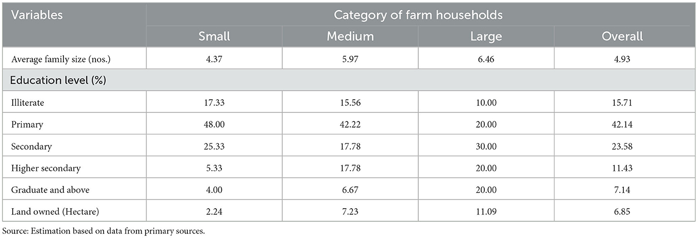
Table 1. Household characteristics among different categories of farm households.

Agriculture in India is a labor-intensive activity and is highly dependent on the family size of farm households. Among the different farm household categories, the family size was found to be highest in the large farm size category, with an average of seven members. Furthermore, the average family size increased with the increase in farm size categories. In the study area, the majority of farm household heads had primary education. Among the farm household categories, the highest proportion of educated farmers was found in the large farm household category (90%), followed by the medium category (84.45%) and the small category (82.67%). The average landholding of the sampled households was found to be 6.85 hectares, with the highest landholding observed in the large farm size category. The categorization of farm households was based on the standard landholding criterion in India.

3.3 Household-level subsidies

Before using the household model, it is important to understand the extent of total and per-unit subsidies received at the farm household level in the study area. The estimation procedure mentioned in the methodology was used to compute the amount of subsidies received by farm households. Subsidies are provided on different inputs to farmers, and the total amount of subsidies received depends on the quantity of inputs used by the farm households (refer to Table 2).

TABLE 2

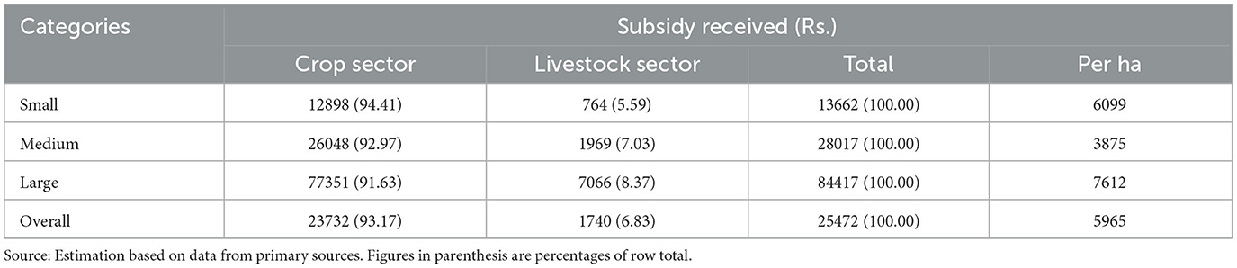
Table 2. Subsidy received among different categories of farm households.

From the table, it can be deduced that the total amount of subsidy received by farm households in the study area was found to be Rs. 25,472 per year, with a per-hectare subsidy of Rs. 5,965. The subsidies on inputs were computed for both the crop and livestock sectors for different farm households, and it can be observed that the crop sector subsidy was approximately more than 10 times that of the livestock subsidy received at the household level. The share of livestock subsidy received at the household level was higher (around 6%) than its share at the national level (<2%) due to the inclusion of only agriculture households with integrated dairy activities in the study. In states such as Punjab and Haryana selected for the study, the livestock production systems are relatively more productive and commercialized, while in most other states, especially in eastern and north-eastern regions, they are primarily subsistence-oriented (Birthal, 2022). Moreover, the concentration of private investment is higher in these states owing to its higher potential.

Farm subsidies account for 2% of India's GDP, with input subsidies forming the highest percentage of farm income at 18.17%, while price support subsidies per hectare account for 2.46% of farm income per hectare.¹ Clearly, the subsidy received at the household level was found to be highest in large farm households. The total subsidy also increased across farm household categories, as the total amount of subsidies received is directly related to the amount of inputs used, representing implicit subsidies. The amount of subsidy received per household was not only the highest in the case of large households in absolute terms but also on a per-hectare basis, indicating a greater dependence of large farms on subsidized inputs. The plausible reason behind it is better linkages with the market and better access to resources. Moreover, large households have more subsidized inputs, which makes them a high bearer of subsidies. The results show that the per-hectare subsidy was found to be the lowest in medium farm households, which may be attributed to their ability to afford inputs and services from private vendors, making them less dependent on subsidized inputs. Table 3 presents the unit of input subsidies received by different categories of farm households.

TABLE 3

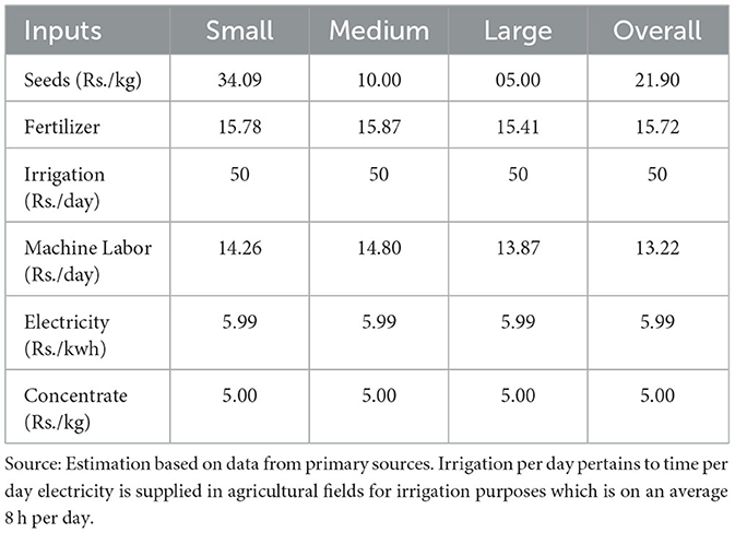
Table 3. Subsidy received per unit of inputs by different categories of farm households.

From the table, it can be clearly seen that the highest per unit subsidy was received for seeds, fertilizer, and irrigation, followed by the machine labor at farm households. These are the results of the primary data collected from 300 farm households. The subsidies received by small and medium farm households were found to be higher as compared to large farm households. Generally, at the farm level, the amount of subsidies received depends on the quantity of inputs used by farm households for the inputs for which subsidies are given implicitly. For more well-off farm households, there will be an increase in the use of inputs, thereby increasing the implicit subsidies. Government policy interventions such as subsidies affect both the consumption and production decisions of farm households. For estimating the effect of this policy intervention, a household model was employed in the study. Empirical estimates of the model are discussed in the following section.

4 Results and discussion

4.1 Empirical results of household model

In a separable approach, these decisions were estimated separately and then integrated through profit. The consumption function of the household was estimated using linear logarithmic expenditure demand systems, and the production approach consisted of using profit function with Cobb-Douglas specification. The demand system consisted of three groups of equations separately for agricultural commodities, non-agricultural commodities, and home time, which were estimated simultaneously with complete demand restrictions as discussed in the methodology. The systems approach permits the imposition of demand theory restrictions and provides more-efficient parameter estimates than a single OLS estimation of each equation (Ahmadi, 1998). The usefulness of the system approach is that it yields maximum likelihood estimates invariant to the equation deleted in the final model estimation (Chalfant, 1987). Since agriculture and non-agriculture commodities are comprised of a number of individual commodities consumed in different quantities, the price indices of these commodities were used instead of actual prices. For the calculation of price indices, expenditure share (Figures 2, 3) on each commodity was computed and multiplied with the price of commodities calculated per household. Figure 2 gives an overview of the average price indices of different commodity groups under different categories of farm households.

FIGURE 2

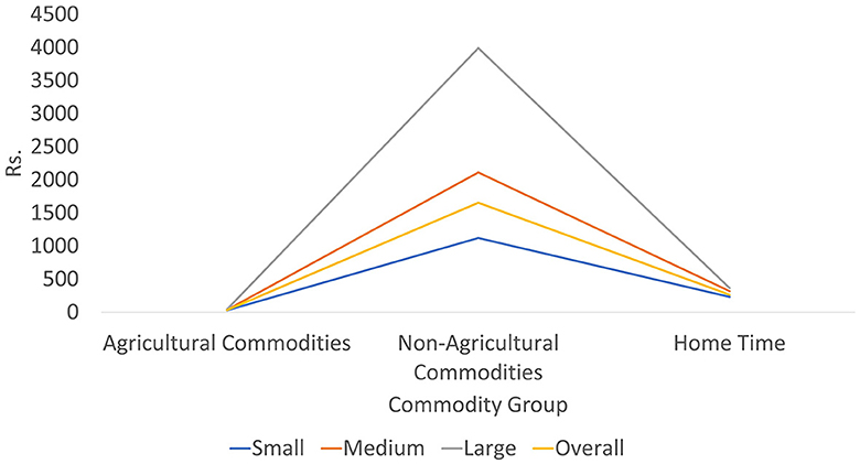
Figure 2. Average price indices of different commodity groups.

FIGURE 3

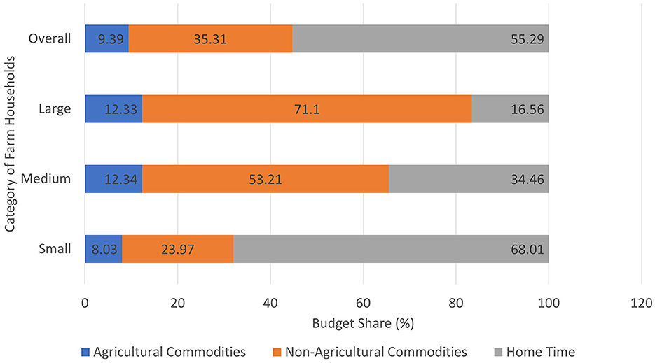
Figure 3. Budget share of different commodity groups (%). Source: estimation based on data from primary sources.

Among farm households, the price indices of both agricultural and non-agricultural commodities increased with an increase in farm size categories due to differences in the quality of the commodities consumed. The figure indicated that in the case of the non-agricultural commodities group, as discussed earlier, the index was higher as compared to the agricultural commodities group. Among farm household categories, the price index was highest for large farm size categories and least for small farm size categories. The percentage of budget share was highest for non-agricultural commodities group in farm size categories except for small farm size categories, and the lowest percentage figures were found for the agricultural commodities group among all farm size categories of households. In the case of small farm size categories, the study revealed that the percentage of budget share was highest for home time group, which comprises 68% of total expenditure. The home time group consists of the imputed value of off-farm work, and its high value reveals that after getting subsidies, small farm size categories had more off-farm work than working on the farm. This poses serious consequences on bringing farmers to the field to avail subsidies and the effectiveness of subsidy programs, especially those that involved cash transfers. The home time group was followed by the non-agricultural commodities group with 23% of the budget share, and the least was found for the agricultural commodities group with 8%. While in medium farm size categories, the highest percentage share was found for the non-agricultural commodities group with 53% of total expenditure, followed by the home time group with 35% of total expenditure, and the least was noted for agriculture commodities group with 12% share of total expenditure. In the case of large farm size categories, the highest percentage share was found for the non-agricultural commodities group with more than half (71%), followed by the home time group with 16%, and the least was again for the agricultural commodities group. This trend of percentage share of budget expenditure explains the general assertion that in India, urbanization and economic growth hassled consumers to find more alternatives in their expenditure decisions. There was a shift in expenditure patterns from agricultural foods such as cereals and pulses to other non-food items. The study by Agbola (2000), using data from the National Sample Survey Organization (NSSO) of India, found similar results where budget share on cereals declined by 38% while the expenditure trend of non-food items was found to be increasing.

4.2 Estimates of linear expenditure systems

The consumption approach of the household model was solved using logarithmic linear expenditure system model estimation, and the results for different farm categories of households in the study area are presented in Table 4.

TABLE 4

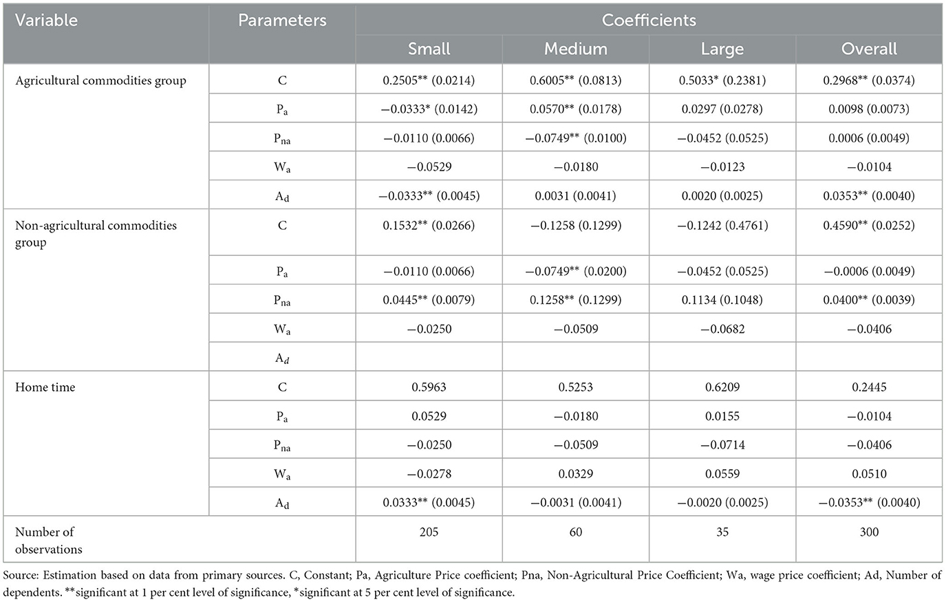
Table 4. Empirical results of linear logarithmic model of consumption with separable household model (price elasticities).

The system of equations was estimated for preferences of consumer behavior for agricultural, non-agricultural, and home time. In the agricultural commodities category, all food items, such as cereals, pulses, meat, and dairy, were taken into account, while in the non-agricultural commodities group, demand for non-agricultural goods, such as electricity, fuel, entertainment, clothing and footwear, medical services, and durable goods and services, were taken into account. The system equations estimation gives more efficient parameter estimates than OLS estimation. The parameters of the omitted equations were estimated using the adding-up theorem. The usefulness of the system approach is that it yields maximum likelihood estimates invariant to the equation deleted in the final model estimation (Chalfant, 1987).

Table 4 depicts a maximum likelihood (ML) estimate for the LES model estimation for different farm household categories. From the perusal of the table, it can be found that for the agriculture group of commodities, the estimated coefficients were positive and <1 for all farm household categories except for the wage-price coefficient, which was found to be negative. The empirical explanation for price elasticities in the logarithmic functional form underlines that when there is a one-percentage change in the price of agricultural commodities, it leads to <1 unit change in demand for agricultural commodities. The results were found to be in conformity with the study of Agbola (2000), in which the price elasticities of food groups were found to be <1. The coefficients were found to be statistically significant for all categories of farmers except large farm households. The price elasticities of other groups were found to be negative, which depicted that the increase in price led to a decrease in demand for the agriculture group of commodities, while none of the coefficients of elasticities were found to be >1. The base explanation for the logarithmic model used for the estimation of price elasticities lies in the positive coefficient indicating that the increase in price led to an increase in demand for the commodity group, whereas the negative value indicates opposite results. Adding to it, each category of consumption varies with permanent income, and the purchase of goods is not correlated to transient income (Deaton and Wigley, 1971).

4.3 Estimates of normalized profit function

Production decisions do not affect the consumption decisions directly, but it depict how a farm chooses its production pattern. For production, different fixed and variable inputs are used for the production of an output. For the analysis of production decisions in a household model, Cobb-Douglas production function was used to estimate the profit function. Variable inputs in the study were labor, irrigation, electricity, fertilizers, seeds, green fodder, dry fodder, etc., while fixed inputs used were capital and land. A farm household aims at maximizing profit on the farm, which is a restricted profit that is assumed to be subject to constraints. In the function, the profit and prices of inputs used were normalized based on output prices. The coefficients of inputs were found using Cobb-Douglas production function. Table 5 gives an overview of coefficients estimated through the production function.

TABLE 5

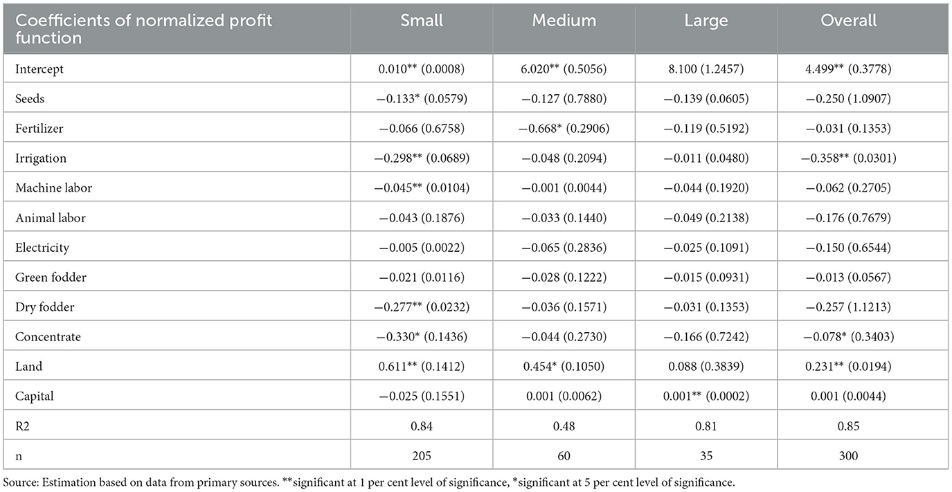
Table 5. Estimates of normalized profit function.

From Table 5, it can be noted that prices of variable inputs generally carried a negative sign showing that they had a negative relation with profit, while fixed inputs had a positive sign depicting a positive relationship with profit. In the research conducted within the study area involving 300 farm households, a significant association was observed between profit and specific factors. Notably, irrigation, concentrate prices, and land inputs displayed distinctive relationships with profit. Irrigation and concentrate prices exhibited negative correlations, whereas the fixed land input demonstrated a positive relationship. In the small farm size category of households, prices of all the variable inputs were found to be having a negative relationship with profit, in which the effect of seeds and manual labor was significant on profit. The coefficients of both irrigation (−0.298) and dry fodder (−0.277) were higher; thus, the magnitude of the effect on profit was also higher. For medium farm households, signs of coefficients of variable inputs were similar to those in small farm households, in which prices of fertilizer were found to be negative and significantly related to profit. In fixed inputs, coefficients of both land and capital were found to be positive, but the land was having a significant effect on the profit of the household. In the large farm size category of households, coefficients of prices of variable inputs had negative signs depicting its negative relationship with profit. In large farm households, the coefficient of capital was found to be positively and significantly related to the profit of households. From the table, it was evident that the use of inputs had a negative relationship with its prices. This relationship was found to be in conformity with study by Komarek et al. (2017) where fertilizer was the input discussed in the study and they found negative association between fertilizer prices and fertilizer used.

4.4 Effect of removal of subsidies on input demand

To trace the effect of subsidies, we have estimated the change in demand for inputs upon the removal of subsidies. The details on the change in absolute demand for different inputs are presented in the Appendix. Table 6 depicts only the percentage change in demand for inputs after the removal of subsidies. From the analysis of the household model, the estimated percentage change in demand after the removal of subsidies depicts that there was a substantial decrease in demand for all the inputs. Overall, the removal of subsidies is going to decrease the demand for electricity, concentrate, and irrigation by 80, 73, and 70%, respectively. From the table, it can be deduced that percent decrease in demand for inputs was lower for large farm households. This implies that the removal of subsidies had more effect on small and medium farm households than large farm households. The plausible reason behind this is the nature of subsidies being given to different categories of farmers, where small farmers were prioritized in the disbursement of subsidies to enhance the use of inputs at the farm level (Deshpande and Reddy, 1992; Sharma and Thaker, 1992; Skaggs and Falk, 1998).

TABLE 6

Table 6. Effects of removal of subsidies on input demand across farm households (% change).

In small farm household demand for machine labor and electricity were found to be having highest percent decrease in demand (−83.54 %) followed by concentrate (−78.05 %) and irrigation (−75.30 %). For other inputs such as seeds and fertilizer, there was a decrease of 62.96 and 67.07% in demand after the removal of subsidies. A perusal of Table 6 unveils that the highest percentage decrease in demand for inputs in medium farm households was seen in the case of demand for electricity, followed by concentrate and irrigation with 86, 81, and 78% decrease. For all the inputs, the percentage decrease in demand was found to be more than 50% in medium farm households. In the case of large farm households, the highest percentage decrease in demand was found for electricity, concentrate, and irrigation, with 60% to 70% decrease, while there was a 30% decrease in the demand for fertilizer after the removal of subsidies. The results find conformity to the study by Druilhe and Barreiro-Hurlé (2012) that if the inputs are being used by households facing market failure, having reduced costs, its demand will increase, thereby increasing the production. But at the local level, farmers need to be aware of the use of these subsidies as it may generate additional demand (Dorward and Chirwa, 2013), certainly which will be reduced if it is removed.

In a separable household model, consumption and production decisions are interlinked with each other through a hinge, i.e., profit. The agricultural household model measures the welfare effect through the interaction of these. Profit is a factor that affects both production and consumption among households. More is the production, hence more is the profit. Table 7 depicts the effects of the removal of subsidies on production, consumption, and marketed surplus of agricultural commodities and the labor supply of farm households.

TABLE 7

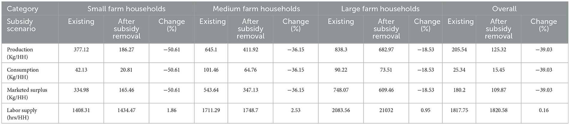
Table 7. Effect of removal of subsidies on household production, consumption and marketed surplus of agricultural commodities and the labor supply (Source: estimation based on data from primary sources).

Withdrawl of all the input subsidies has registered a 39% decline in the production, consumption, and marketed surplus of agricultural produce. However, labor supply has increased. It can be observed from the withdrawal of subsidy that the production of agricultural commodities will reduce from 205.54 kg to 125.32 kg per household. A similar effect can be seen in consumption and marketed surplus of agricultural commodities. It is to be noted that the reduction in all three factors (production, consumption, and marketed surplus) was found to be highest in small farm households, i.e., around −50%, followed by medium farm households (−36.15%) and large households (−18.53%). The results were found in line with the results that farmers may enter into a savings mode since they have access to subsidized inputs without any increase in farm productivity, which may be true in large farm household category (Kato and Greeley, 2016). There was a noted effect of the removal of subsidies not only on the consumption of staple food but also on the non-food items, and thus, the results were found in line with available literature (Rosegrant and Kasryno, 1991; Stifel and Randrianarisoa, 2004).

Nevertheless, the percentage change in labor supply was found to have increased. It is convinced that the removal of subsidies will lead to a decrease in demand for home time because in the absence of subsidy, farmers are to work more to maintain their income level, which ultimately increases the labor supply. Home time is an off-farm time spent by an individual in meeting his household social, personal, and family requirements. Leisure is assumed to be a normal good, and an increase in income through government payments will lead to an increase in unambiguous leisure and a decrease in work time. A thorough analysis of Table 7 states that when there is a removal of subsidy on inputs given to farm households, there is a decrease in demand for home time while the labor supply increased. Basically, a household confronts constraints in deciding how much time to devote to on-farm, off-farm, and leisure. Diminishing marginal factor productivity of farm household labor plays a role in deciding how much time to devote on-farm vs. off-farm work. Although the overall percentage change in labor supply was negligible (0.16%), it was found to be highest in the case of medium farm households (2.53%), followed by small households (1.86%), and the least percentage increase was noted for large farm households (0.95%). There were varied results claiming both positive and negative association of government payments with labor supply in the literature. On one hand, Dewbre and Mishra (2007) found that payments tend to increase the time allocated to leisure as the effect of payments mainly depends on intra-household time allocation. While, on the other hand, the study by Mishra and Goodwin (1997), found that such payments reduced off-farm work since they provided an additional source of income to farmers, thus decreasing off-farm employment.

5 Conclusion

Our results provide insights to the effects of the removal of subsidies as it is likely to have serious implications not only on the production side but also on consumption at the farm household level. Studies using household model have not been conducted in India using cross-sectional data, so our study is a novel approach in this regard. Nevertheless, we cannot deny the fact that there is a constraint of having a sophisticated database. Adding to the limitations of the study, it may have few prior studies for comparable studies to draw upon. Moreover, the study does not fully explore the regional subsidy programs or potential alternative policies. The study paves a future path for research on subsidies to trace its trajectory with clear policy outcomes. Earlier studies have indeed concluded subsidies to be unsustainable in the long run, but we emphasize that complete removal may lead to food insecurity and a decreased standard of living for farmers. This is the reason behind direct benefit transfer started by the government, which is evolving and eventually falling into place. It may be due to the fact that subsidies are targeted at input price and input use. Subsidies on inputs, such as fertilizers, seeds, implements, and irrigation, are implicit subsidies and less use of these inputs infers that small and marginal farmers in the study area were less likely to be benefitted from subsidies. This was primarily due to the untargeted input subsidies, which benefit farmers who are using it more, often the large farmers. On the other hand, output prices are less remunerative to bear the effect of removal of subsidy and ultimately reduce the profit and income of the household. Consumption and production decisions are interlinked with each other, though the hinge, i.e., profit and the welfare effect is measured through the interaction of these. The empirical findings of the household model depict that removal of subsidies will not only affect the demand for inputs but will also lead to a decline in the demand for consumption of both agricultural and non-agricultural commodities. The effect of removal of subsidies was found to be more prominent in small and medium farm households, which implies these households were prioritized while channeling the subsidies. This underscores the importance attached to Direct Benefit Transfer (DBT) to the small and marginal farmers. Moreover, the study may help in tracking leakage and environmental damage caused due to overuse of subsidies. Thus, with proper planning, clear policy outcomes, and long-term vision, further research to document both primary and secondary outcomes of subsidies in India needs to be done to decide upon a structured course of action for subsidy distribution.

Data availability statement

The original contributions presented in the study are included in the article/Supplementary material, further inquiries can be directed to the corresponding authors.

Author contributions

PL: Data curation, Formal analysis, Conceptualization, Investigation, Methodology, Writing – original draft. BC: Conceptualization, Supervision, Writing – review & editing. RT: Writing – review & editing, Data curation, Methodology. ME-S: Writing – review & editing, Data curation, Formal analysis, Funding acquisition. SM: Writing – review & editing, Methodology, Formal analysis, Funding acquisition. AK: Writing – original draft, Conceptualization, Formal analysis, Validation, Visualization. GS: Writing – review & editing, Data curation, Investigation, Visualization. ML: Data curation, Writing – review & editing, Software. RK: Data curation, Writing – review & editing, Formal analysis.

Funding

The author(s) declare that no financial support was received for the research, authorship, and/or publication of this article.

Acknowledgments

The authors extend their appreciation to the Researchers Supporting Project number (RSP2023R182), King Saud University, Riyadh, Saudi Arabia.

Conflict of interest

The authors declare that the research was conducted in the absence of any commercial or financial relationships that could be construed as a potential conflict of interest.

The author(s) declared that they were an editorial board member of Frontiers, at the time of submission. This had no impact on the peer review process and the final decision.

Publisher's note

All claims expressed in this article are solely those of the authors and do not necessarily represent those of their affiliated organizations, or those of the publisher, the editors and the reviewers. Any product that may be evaluated in this article, or claim that may be made by its manufacturer, is not guaranteed or endorsed by the publisher.

Supplementary material

The Supplementary Material for this article can be found online at: https://www.frontiersin.org/articles/10.3389/fsufs.2023.1295704/full#supplementary-material

Footnotes

1. ^Chandrakanth, M. G. (2021). Available online at: https://timesofindia.indiatimes.com/blogs/author/prof-mg-chandrakanth/.

References

Acharya, S. (2000). Subsidies in Indian agriculture and their beneficiaries. Agric. Sit. India 57, 251–260.

Google Scholar

Agbola, F. (2000). Estimating the Demand for Food and Non-Food Items Using an Almost Ideal Demand System Modelling Approach. Sydney: Australian Agricultural and Resource Economics Society, 1–14.

Google Scholar

Ahearn, M., El-Osta, H., and Dewbre, J. (2006). The impact of coupled and decoupled government subsidies on off-farm labor participation of U.S. farm operators. Am. J. Agric. Econ. 88, 393–408. doi: 10.1111/j.1467-8276.2006.00866.x

CrossRef Full Text | Google Scholar

Ahmadi, E. (1998). The Wholesale Demand for Food in China: An Economic Analysis of the Implications for Australia. Canberra, ACT: Rural Industries Research and Development Corporation.

Google Scholar

Bergström, F. (2000). Capital subsidies and the performance of firms. Small Bus. Econ. 14, 183–193. doi: 10.1023/A:1008133217594

CrossRef Full Text | Google Scholar

Bezlepkina, I. V., and Oude Lansink, A. (2006). Impact of debts and subsidies on agricultural production: Farm-data evidence. Q. J. Int. Agric. 45, 7–34.

Google Scholar

Birthal, P. S. (2022). Livestock, Agricultural Growth and Poverty Alleviation. NABARD Research and Policy Series No.7/2022. Mumbai: National Bank for Agriculture and Rural Development, Mumbai.

Google Scholar

Chalfant, J. (1987). A globally flexible, almost ideal demand system. J. Bus. Econ. Stat. 5, 233–242. doi: 10.1080/07350015.1987.10509581

CrossRef Full Text | Google Scholar

Deaton, A. S., and Wigley, K. J. (1971). Econometric models for the personal sector. Bullet. Oxford Univ. Inst. Econ. Stat. 33, 81–91. doi: 10.1111/j.1468-0084.1971.mp33002001.x

CrossRef Full Text | Google Scholar

Deshpande, R., and Reddy, V. (1992). Impact of Subsidies on Agricultural Development. Pune: Agro Economic Research Centre, Gokhale Institute of Politics and Economics.

Google Scholar

Dewbre, J., and Mishra, A. K. (2007). Impact of program payments on time allocation and farm household income. J. Agric. Appl. Econ. 39, 489–505. doi: 10.1017/S1074070800023221

CrossRef Full Text | Google Scholar

Dorward, A. R., and Chirwa, E. W. (2013). Impacts of the Farm Input Subsidy Programme in Malawi: Informal Rural Economy Modelling. Future Agricultures Consortium Working Paper, 067.

Google Scholar

Druilhe, Z., and Barreiro-Hurlé, J. (2012). Fertilizer Subsidies in Sub-Saharan Africa, ESA Working Paper No. 12–04. Rome: FAO.

Google Scholar

Ellis, F. (1988). Peasant Economics: Farm Households and Agrarian Development. Cambridge: Cambridge University Press.

Google Scholar

El-Osta, H. S., Mishra, A. K., and Ahearn, M. C. (2004). Labor supply by farm operators under 'decoupled' farm program payments. Rev. Econ. Household 2, 367–385. doi: 10.1007/s11150-004-5653-7

CrossRef Full Text | Google Scholar

Fan, S., Gulati, A., and Thorat, S. (2009). Investment, subsidies, and pro-poor growth in rural India. Agric. Econ. 39, 163–170. doi: 10.1111/j.1574-0862.2008.00328.x

CrossRef Full Text | Google Scholar

Garg, B., and Dhaliwal, N. (1982). Rationale for subsidy for dairying in Punjab. Indian J. Agric. Econ. 37, 280.

Google Scholar

Giannakas, K., Schoney, R., and Tzouvelekas, V. (2001). Technical effciency, technological change and output growth of wheat farms in Saskatchewan. Can. J. Agric. Econ. 49, 135–152. doi: 10.1111/j.1744-7976.2001.tb00295.x

CrossRef Full Text | Google Scholar

Guan, Z., and Oude Lansink, A. (2006). The source of product in Dutch agriculture – a perspective from finance. Am. J. Agric. Econ. 88, 644–656. doi: 10.1111/j.1467-8276.2006.00885.x

CrossRef Full Text | Google Scholar

Gulati, A. (1990). Fertilizer Subsidy: Is the cultivator “net subsidized”. Indian J. Agric. Econ. 45, 1–10.

Google Scholar

Hadley, D. (2006). Patterns in technical effciency and technical change at the farm-level in England and Wales, 1982–2002. J. Agric. Econ. 57, 81–100. doi: 10.1111/j.1477-9552.2006.00033.x

CrossRef Full Text | Google Scholar

Henningsen, A., Kumbhakar, S., and Lien, G. (2009). Econometric Analysis of the Effects of Subsidies on Farm Production in Case of Endogenous Input Quantities. Selected Paper Prepared for Presentation at the Agricultural and Applied Economics Association, 26–29. Available online at: http://ageconsearch.umn.edu/bitstream/49728/2/Henningsen_Kumbhakar_Lien_2.pdf (accessed April 1, 2017).

Google Scholar

Jayne, T. S., and Rashid, S. (2013). Input subsidy programs in sub-Saharan Africa: a synthesis of recent evidence. Agric. Econ. 44, 547–562. doi: 10.1111/agec.12073

CrossRef Full Text | Google Scholar

Jones, C. (2013). Subsidies in the Global Food System I: India's Subsidised Farm Inputs - Future Directions International. Available online at: https://www.futuredirections.org.au/publication/subsidies-in-the-global-food-system-i-india-s-subsidised-farm-inputs/ (accessed June 4, 2021).

Google Scholar

Karagiannis, G., and Sarris, A. (2005). Measuring and explaining scale efficiency with the parametric approach: the case of Greek tobacco growers. Agric. Econ. 33, 441–451. doi: 10.1111/j.1574-0864.2005.00084.x

CrossRef Full Text | Google Scholar

Kato, T., and Greeley, M. (2016). Agricultural input subsidies in sub-saharan africa. IDS Bulletin 47, 130. doi: 10.19088/1968-2016.130

CrossRef Full Text | Google Scholar

Khonje, M., Nyondo, C., Mangisoni, J. H., Ricker-Gilbert, J., Burke, W. J., Chadza, W., et al. (2021). Does subsidizing legume seeds improve farm productivity and nutrition in Malawi? Food Policy 113, 102308. doi: 10.1016/j.foodpol.2022.102308

CrossRef Full Text | Google Scholar

Kleinhanß, W., Murillo, C., Juan, C. S., and Sperlich, S. (2007). Efficiency, subsidies, and environmental adaption of animal farming under CAP. Agric. Econ. 36, 49–65. doi: 10.1111/j.1574-0862.2007.00176.x

CrossRef Full Text | Google Scholar

Komarek, A. M., Drogue, S., Chenoune, R., Hawkins, J., Msangi, S., Belhouchette, H., et al. (2017). Agricultural household effects of fertilizer price changes for smallholder farmers in central Malawi. Agric. Syst. 154, 168–178. doi: 10.1016/j.agsy.2017.03.016

CrossRef Full Text | Google Scholar

McCloud, N., and Kumbhakar, S. C. (2008). Do subsidies drive product? a cross-country analysis of Nordic dairy farms. Adv. Econ. 23, 1–14. doi: 10.1016/S0731-9053(08)23008-2

CrossRef Full Text | Google Scholar

Mishra, A. K., and Goodwin, B. K. (1997). Farm income variability and the supply of off-farm labor. Am. J. Agric. Econ. 79, 880–887. doi: 10.2307/1244429

CrossRef Full Text | Google Scholar

Narayanamoorthy, A. (1997). Economic viability of drip irrigation: an empirical analysis from Maharashtra. Ind. J. Agric. Econ. 52, 728–739.

Google Scholar

Pandey, U., and Khanna, S. (1980). An economic evaluation of small farmers' development agency for weaker sections in Haryana. Ind. J. Agric. Econ. 35, 49–58.

Google Scholar

Piesse, J., and Thirtle, C. (2000). A stochastic frontier approach to firm level efficiency, technological change and productivity during early transition in Hungary. J. Comp. Econ. 28, 473–501. doi: 10.1006/jcec.2000.1672

CrossRef Full Text | Google Scholar

Rizov, M., Pokrivcak, J., and Ciaian, P. (2013). CAP subsidies and productivity of the EU farms. J. Agric. Econ. 64, 537–557. doi: 10.1111/1477-9552.12030

CrossRef Full Text | Google Scholar

Rosegrant, M. W., and Kasryno, F. (1991). The impact of fertilizer subsidies and rice price policy on food crop production in Indonesia. ACIAR Proc. Series 12, 32–41.

Google Scholar

Ruzzante, S., Labarta, R., and Bilton, A. (2021). Adoption of agricultural technology in the developing world: a meta-analysis of the empirical literature. World Dev. 146, 105599. doi: 10.1016/j.worlddev.2021.105599

CrossRef Full Text | Google Scholar

Sadoulet, E., and de Janvry, A. (1995). Household Models. Quantitative Development Policy Analysis. London: The John Hopkins University Press.

Google Scholar

Sharma, V. P., and Thaker, H. (1992). Fertilizer subsidy in India: Who are the beneficiaries? Econ. Polit. Weekly 45, 68–76.

Google Scholar

Skaggs, R. K., and Falk, C. L. (1998). Market and welfare effects of livestock feed subsidies in Southeastern New Mexico. J. Agric. Res. Econ. 23, 545–557.

Google Scholar

Skuras, D., Tsekouras, K., Dimara, E., and Tzelepis, D. (2006). The effects of regional capital subsidies on productivity growth: a case study of the Greek food and beverage manufacturing industry. J. Reg. Sci. 46, 355–381. doi: 10.1111/j.0022-4146.2006.00445.x

CrossRef Full Text | Google Scholar

Stifel, D., and Randrianarisoa, J C. (2004). Rice Prices, Agricultural Input Subsidies, Transactions Costs and Seasonality: A Multi-Market Model Poverty and Social Impact Analysis PSIA for Madagascar. Washington, DC: World Bank

Google Scholar

Stone, J. (1954). Linear expenditure systems and demand analysis: an application to the pattern of british demand. Econ. J. 64, 511–527. doi: 10.2307/2227743

CrossRef Full Text | Google Scholar

Subramanian, R., Kakkagowder, C., Perumal, A., and Gurusamy, P. (2019). Consumption, expenditure and demand analysis of milk and milk products in India. Ind. J. Econ. Dev. 15, 301–306. doi: 10.5958/2322-0430.2019.00037.4

CrossRef Full Text | Google Scholar

Yadav, S., Singh, S., and Dubey, A. (1982). Role of subsidy in agricultural development. Ind. J. Agric. Econ. 37, 278–279.

Google Scholar

Zellner, A. (1962). An efficient method of estimating seemingly unrelated regression equations and tests for aggregation bias. J. Am. Stat. Assoc. 57, 348–368. doi: 10.1080/01621459.1962.10480664

CrossRef Full Text | Google Scholar