Green total factor productivity growth and its driving forces in China’s fisheries sector

The rapid development of China’s fisheries sector has brought about significant environmental problems, which are detrimental to the sustainable development of the sector. Balancing environmental protection while promoting fisheries development has become an urgent issue in China. Based on data from 30 provincial-level administrative regions in China from 2004 to 2019, this study utilizes the Epsilon-based Measure (EBM) model considering undesirable outputs and the global Malmquist-Luenberger (GML) index to measure the green total factor productivity (GTFP) growth in China’s fisheries sector. Furthermore, it explores the spatiotemporal evolution and driving forces of fisheries GTFP growth using spatial Durbin model (SDM). The results indicate that ignoring the resource and environmental costs in fisheries production would overestimate the growth of total factor productivity (TFP) by 1.3%. The growth of fishery output primarily comes from the increase in input factors, exhibiting extensive characteristics that have been gradually diminishing over time. During the sample period, the provinces with the fastest growth in GTFP shifted from being mainly concentrated in the central and western regions to the eastern region. The local driving forces behind the improvement of fisheries GTFP include internet penetration rate, transportation convenience, education level of rural residents. The driving forces from economically similar provinces include the positive spatial interplay between provinces, fishery disaster rate, fisherman training, fishery trade openness, and urbanization rate. Overall, these finds offer a novel approach to reexamine the growth of China’s fisheries and provide valuable insights for the future fisheries development.

1. Introduction

TFP has received significant research attention in the literature on economic growth as a driving force for economic development beyond input factors (Solow, 1957; Pan et al., 2022). In the field of fisheries research, TFP has also been the subject of significant focus and is commonly used to measure the quality of fisheries development (Asche et al., 2013; Aponte, 2020; Zhong et al., 2022). Therefore, improving the TFP of the fisheries sector has become one of the key issues for achieving high-quality development. However, in the face of resource and environmental challenges in fisheries development, it is not enough to focus solely on improving TFP. Prolonged extensive development in the fisheries sector has led to severe resource and environmental problems. In response, the Chinese government has introduced a series of laws and regulations to promote sustainable fisheries development. In 2013, the State Council issued “Several Opinions on Promoting the Sustainable and Healthy Development of Marine Fisheries,” which emphasized the protection of marine fishery resources and the ecological environment. With a focus on aquaculture, the Ministry of Agriculture and Rural Affairs, the Ministry of Ecology and Environment, and other departments jointly issued “Several Opinions on Accelerating the Green Development of Aquaculture” in 2019, which outlined the direction for the green development of the aquaculture industry from various perspectives such as spatial layout, farming methods, and environmental considerations. Considering the current situation of fisheries development and policy directions, green development will be the primary direction for the future of China’s fisheries. The measurement and analysis of GTFP in the fisheries sector take into account the costs of resources and environmental factors, thus reflecting the resource and environmental constraints faced in fisheries development. Therefore, assessing and analyzing fisheries GTFP is of significant importance in promoting sustainable development in the industry.

Currently, research on TFP in the fishing industry focuses on two main aspects. The first aspect is the measurement and analysis of fisheries TFP. The measurement can be broadly classified into two categories: parametric estimation and non-parametric estimation (Ye et al., 2023). Parametric estimation is primarily based on production functions and involve estimating residuals from the production function relationship to measure TFP (Van Beveren, 2012; Van Nguyen and See, 2023). In the fishing industry, it is more common to combine production functions with Törnqvist index to measure total factor productivity (Squires, 1992; Wang and Walden, 2021). Non-parametric estimation primarily refers to the combined use of data envelopment analysis (DEA) and the malmquist index (Asche et al., 2013; Zhang et al., 2023). When looking at specific sectors, the measurement of TFP in the fishing sector is mostly estimated using parametric methods. For example, Wang and Walden (2021) used a constructed production function to measure the TFP of the US commercial fishing industry. They found that improvements in biomass growth can lead to higher output growth or lower input growth. In the aquaculture sector, both parametric and non-parametric methods are commonly used in research for measuring TFP. Indeed, there is a temporal sequence in the application of these two measurement methods in the aquaculture sector (See et al., 2021). In the early stages of research, the focus was primarily on using stochastic frontier analysis, such as the stochastic logarithmic production function, to measure technical efficiency, an important component of TFP in aquaculture. It was only later that studies began to incorporate the use of DEA for TFP estimation. Both measurement methods have their respective advantages, and the choice of which method to use depends on factors such as research objectives, data, production process type, and numbers of output (Pascoe and Tingley, 2007; Van Nguyen et al., 2021). This study will utilize an evolved methodology based on DEA, known as EBM, in conjunction with the GML index, to measure the GTFP growth in China’s fisheries sector. Additionally, it is important to emphasize that the fisheries sector mentioned in this study refers to both aquaculture and fishing sectors.

Another type of research focuses on explaining the factors causing changes in fisheries TFP. These factors involve specific policies, fleet characteristics, environmental and farm characteristics, but they exhibit variations in the fishing and aquaculture sectors. In the fishing sector, fishery resource management policies are crucial (McClanahan et al., 2015). These fishery resource management policies primarily focus on the management of fisheries capture and vessels, such as individual fishing quotas (Sanchirico et al., 2006; Solís et al., 2014), transferable quotas (Newell et al., 2005; Pincinato et al., 2021), Vessel Capacity Reduction Programs (Holland et al., 1999, 2017). Among these, most studies have affirmed the positive effects of these policies on fishing vessel TFP (Pascoe et al., 2012; Solís et al., 2015; Nielsen et al., 2023), while a few studies have found that some policies have not achieved the intended outcomes (Walden et al., 2012). Additionally, factors such as total kW, total fishing days per year, and the stock of physical capital also influence vessel TFP (Jin et al., 2002; Pipitone and Colloca, 2018). In comparison to the fishing sector, there are more factors that affect the TFP in the aquaculture sector. These factors include education level, experience, age and credit constraints of the farmer (Kareem et al., 2009; Iliyasu et al., 2016; Mitra et al., 2019; See et al., 2021), adoption of new production technology or production process innovation (Dey et al., 2010), pond characteristics (Long et al., 2020; Mitra et al., 2020), family characteristics (Iliyasu et al., 2016), and government regulations (Shao et al., 2021).

In this study, the GTFP of the fisheries sector was measured, and subsequently, its driving forces were explored. This study contributes to existing research in three aspects. Firstly, previous studies have mainly focused on either the fishing or aquaculture sector, and often explored the total factor productivity (TFP) of specific fish species production, which fails to provide a comprehensive view of the TFP of the entire fisheries sector. This study combines the fishing and aquaculture sectors to investigate the overall TFP of the fisheries sector. Secondly, it departs from the traditional understanding of fisheries growth, shifting from a focus on productivity growth to a balance between productivity growth and sustainable resource-environment considerations. Previous studies on fisheries productivity often neglected the environmental externalities associated with fishing activities. This study takes into account the environmental costs associated with fisheries production in calculating the TFP. Additionally, considering the carbon sequestration function of fisheries, the study incorporates the economic value of carbon sequestration in desirable outputs. Thirdly, this study analyzes the driving forces of fisheries GTFP based on five dimensions: natural environment, infrastructure, human capital, market size, and government governance. It also explores the spatial spillover effects of these dimensions on fisheries GTFP.

The rest of the paper is organized as follows. Section 2 provides theoretical analysis and proposes relevant hypotheses. Section 3 introduces the methodology, indicator selection and data sources. Results are presented in Section 4. Section 5 summarizes the conclusions and provides policy implications.

2. Methods and materials

2.1. Measuring GTFP growth for the fishery sector

By utilizing input and output data, DEA can be used to evaluate the efficiency of decision-making units. DEA primarily consists of two types: radial measurement-based models and non-radial measurement-based models. Radial measurement-based models do not consider slack variables and assume that all factors change proportionally. However, this assumption does not align with reality. Non-radial measurement-based models incorporate slack variables and avoid the strict assumptions of radial measurement by identifying points that are far from the frontier to maximize input and output inefficiency. This means that the original ratio information of the efficiency frontier projection is lost. To address the issues faced in non-radial measurement, Tone and Tsutsui (2010) proposed the EBM in 2010. Based on this model, and following the approach of Wu et al. (2019), we have developed an EBM that incorporates undesirable outputs. The formula is as follows:

$\begin{array}{ll}{\mathrm{k}}^{\ast }=\underset{\theta ,\eta ,\lambda ,{\mathrm{s}}^{-},{\mathrm{s}}^{+\mathrm{g}},{\mathrm{s}}^{-\mathrm{b}}}{min}\frac{\theta -{\epsilon }_{\mathrm{x}}{{\displaystyle \sum }}_{\mathrm{i}=1}^{\mathrm{m}}\frac{{\mathrm{w}}_{\mathrm{i}}^{-}{\mathrm{s}}_{\mathrm{i}}^{-}}{{\mathrm{x}}_{\mathrm{i}0}}}{\eta +{\epsilon }_{\mathrm{y}}\left[{{\displaystyle \sum }}_{\mathrm{i}=1}^{\mathrm{s}1}\frac{{\mathrm{w}}_{\mathrm{i}}^{+\mathrm{s}1}{\mathrm{s}}_{\mathrm{i}}^{+\mathrm{g}}}{{\mathrm{y}}_{\mathrm{i}0}}+{{\displaystyle \sum }}_{\mathrm{i}=1}^{\mathrm{s}2}\frac{{\mathrm{w}}_{\mathrm{i}}^{-\mathrm{s}2}{\mathrm{s}}_{\mathrm{i}}^{-\mathrm{b}}}{{\mathrm{y}}_{\mathrm{i}0}}\right]}& (1)\end{array}$

$\mathrm{s}.\mathrm{t}.\{\begin{array}{c}\hfill \theta {\mathrm{X}}_0-X\lambda -{\mathrm{s}}^{-}=0\hfill \\ \hfill \begin{array}{c}\hfill \eta {\mathrm{Y}}_0-{\mathrm{Y}}^{+\mathrm{g}}\lambda +{\mathrm{s}}^{+\mathrm{g}}=0\hfill \\ \hfill \eta {\mathrm{Y}}_0-{\mathrm{Y}}^{-\mathrm{b}}\lambda -{\mathrm{s}}^{-\mathrm{b}}=0\hfill \end{array}\hfill \\ \hfill \begin{array}{c}\hfill {\lambda }_1+{\lambda }_2+\dots +{\lambda }_{\mathrm{n}}=1\hfill \\ \hfill \lambda \ge 0,{\mathrm{s}}^{-}\ge 0,{\mathrm{s}}^{+\mathrm{g}}\ge 0,{\mathrm{s}}^{-\mathrm{b}}\ge 0,\theta \le 1,\eta \le 1\hfill \end{array}\hfill \end{array}$

Where $s^{-}$ represents the slack variable. $s^{+g}$ and $s^{-b}$ are both redundant variables. $W_i^{-}$ represents the weight of the i-th input, with $\sum W_i^{-}=1$ ( ${\forall }_i{W}_i^{-}\ge 0$ ). $W_i^{+}$ represents the weight of the s-th output, with $\sum W_i^{+S1}+\sum W_i^{-S2}=1$ ( ${\forall }_i{W}_i^{+}\ge 0$ ).

Relying solely on the EBM model is insufficient for measuring fisheries GTFP growth; the use of index methods is also necessary. The Malmquist-Luenberger (ML) index has long been used to measure productivity growth incorporating undesirable outputs. However, this index can encounter cases where linear programming has no solution and suffer from non-transitivity issues. To overcome the limitations of the ML index, Oh (2010) proposed the GML index. This study considers the combination of the EBM model with the GML index, incorporating undesirable outputs, to measure China’s fisheries GTFP growth. Existing studies decomposes the GML index into two dimensions: efficiency change and technological change. The formula for the GML index is as follows:

$\begin{array}{ll}{\mathrm{G}\mathrm{M}\mathrm{L}}^{\mathrm{t},\mathrm{t}+1}\left({\mathrm{x}}^{\mathrm{t}},{\mathrm{y}}^{\mathrm{t}},{\mathrm{b}}^{\mathrm{t}},{\mathrm{x}}^{\mathrm{t}+1},{\mathrm{y}}^{\mathrm{t}+1},{\mathrm{b}}^{\mathrm{t}+1}\right)=\frac{1+{\mathrm{D}}^{\mathrm{G}}\left({\mathrm{x}}^{\mathrm{t}+1},{\mathrm{y}}^{\mathrm{t}+1},{\mathrm{b}}^{\mathrm{t}+1}\right)}{1+{\mathrm{D}}^{\mathrm{G}}\left({\mathrm{x}}^{\mathrm{t}},{\mathrm{y}}^{\mathrm{t}},{\mathrm{b}}^{\mathrm{t}}\right)}& (2)\end{array}$

$\begin{array}{l}=\frac{1+{\mathrm{D}}^{\mathrm{t}+1}\left({\mathrm{x}}^{\mathrm{t}+1},{\mathrm{y}}^{\mathrm{t}+1},{\mathrm{b}}^{\mathrm{t}+1}\right)}{1+{\mathrm{D}}^{\mathrm{t}}\left({\mathrm{x}}^{\mathrm{t}},{\mathrm{y}}^{\mathrm{t}},{\mathrm{b}}^{\mathrm{t}}\right)}\\ \times \left(\frac{\left(1+{\mathrm{D}}^{\mathrm{G}}\left({\mathrm{x}}^{\mathrm{t}+1},{\mathrm{y}}^{\mathrm{t}+1},{\mathrm{b}}^{\mathrm{t}+1}\right))/(1+{\mathrm{D}}^{\mathrm{t}+1}\left({\mathrm{x}}^{\mathrm{t}+1},{\mathrm{y}}^{\mathrm{t}+1},{\mathrm{b}}^{\mathrm{t}+1}\right)\right)}{\left(1+{\mathrm{D}}^{\mathrm{G}}\left({\mathrm{x}}^{\mathrm{t}},{\mathrm{y}}^{\mathrm{t}},{\mathrm{b}}^{\mathrm{t}}\right)/(1+{\mathrm{D}}^{\mathrm{t}}\left({\mathrm{x}}^{\mathrm{t}},{\mathrm{y}}^{\mathrm{t}},{\mathrm{b}}^{\mathrm{t}}\right)\right)}\right)\end{array}$

$={\mathrm{E}\mathrm{C}}^{\mathrm{t},\mathrm{t}+1}\times {\mathrm{T}\mathrm{C}}^{\mathrm{t},\mathrm{t}+1}$

Where $D^t\left(x^t,y^t,b^t\right)$ and $D^G\left(x^t,y^t,b^t\right)$ represent the current and global EBM directional distance function, respectively. $b^t$ represents the undesirable output of the decision-making unit in period t. $GM{L}^{t,t+1}$ represents the growth in fisheries GTFP from period t to t + 1. $E{C}^{t,t+1}$ represents the change in efficiency from period t to t + 1, and $T{C}^{t,t+1}$ represents the change in technology from period t to t + 1. When $GM{L}^{t,t+1}$ , $E{C}^{t,t+1}$ , and $T{C}^{t,t+1}$ are greater than 1, it indicates growth from period t to t + 1. If they are equal to 1, it means no change, and if they are less than 1, it indicates a decline.

2.2. Methods for testing the drivers of fisheries GTFP growth

This study will employ spatial econometric model to examine the drivers of fisheries GTFP growth. Spatial econometric model is advantageous as it can effectively handle the spatial correlation among spatial units and test the spatial spillover effects. Prior to estimating the spatial econometric model, it is necessary to test the spatial autocorrelation of the dependent variable to determine the need for employing spatial econometric model. In this study, the Global Moran’s I index will be used to test the spatial autocorrelation of fisheries GTFP growth. The expression for the Global Moran’s I index is as follows:

$\begin{array}{ll}{\mathrm{Moran}}^{\text{'}}\mathrm{s}\mathrm{I}=\frac{{{\displaystyle \sum }}_{\mathrm{i}=1}^{\mathrm{n}}{{\displaystyle \sum }}_{\mathrm{j}=1}^{\mathrm{n}}{\mathrm{W}}_{\mathrm{i}\mathrm{j}}\left({\mathrm{Y}}_{\mathrm{i}}-\overline{Y}\right)\left({\mathrm{Y}}_{\mathrm{j}}-\overline{Y}\right)}{{\mathrm{S}}^2{{\displaystyle \sum }}_{\mathrm{i}=1}^{\mathrm{n}}{{\displaystyle \sum }}_{\mathrm{j}=1}^{\mathrm{n}}{\mathrm{W}}_{\mathrm{i}\mathrm{j}}},\left(\mathrm{i}\ne \mathrm{j}\right)& (3)\end{array}$

${\mathrm{S}}^2=\frac{{{\displaystyle \sum }}_{\mathrm{i}=1}^{\mathrm{n}}{\left({\mathrm{Y}}_{\mathrm{i}}-\overline{Y}\right)}^2}{\mathrm{n}}$

Where $Y_i$ and $Y_j$ represent the fisheries GTFP growth of province i and province j, respectively. $W_{ij}$ is the spatial weight matrix based on inverse economic distance, which captures the interconnections between provinces. The value of the Moran’s I index is between 0 and 1. A positive Moran’s I index indicate the presence of spatial autocorrelation in fisheries GTFP, implying that high values tend to cluster with high values and low values tend to cluster with low values. Conversely, a negative Moran’s I index suggests the existence of spatial heterogeneity, where high values (low values) tend to cluster with low values (high values). When Moran’s I index equal to zero, it signifies the absence of spatial correlation, indicating a random distribution of fisheries GTFP growth among provinces. Spatial correlation represents a form of spatial dependence, reflecting the first law of geography, which states that geographically proximate entities are more likely to be related.

If the estimation of the Global Moran’s I index suggests the presence of spatial correlation in fisheries GTFP growth, it is essential to employ spatial econometric models to examine the driving factors of this productivity. The three classical specifications of spatial econometric models are the SDM, spatial autoregressive model (SAR), and spatial error model (SEM). To determine the appropriate model specification among these, it is common practice to conduct tests using the SDM as the baseline model and employing the WALD, LR, and LM tests. In this study, the SDM specification is as follows:

$\begin{array}{ll}{\mathrm{FGTFP}}_{\mathrm{it}}=\rho W\ast {\mathrm{FGTFP}}_{\mathrm{j}\mathrm{t}}+\alpha X_{\mathrm{it}}+\beta W\ast {\mathrm{X}}_{\mathrm{j}\mathrm{t}}+{\gamma }_{\mathrm{i}}+{\phi }_{\mathrm{t}}+{\mu }_{\mathrm{it}}& (4)\end{array}$

Where $\mathit{FGTF}{P}_{\mathit{it}}$ denotes the fisheries GTFP growth of province i in year t. $W\ast \mathit{FGTF}{P}_{jt}$ represents the spatial lag term of fisheries GTFP growth, and the corresponding coefficient $\rho$ captures the strength of spatial interaction among provinces regarding GTFP growth. $X_{\mathit{it}}$ represents the vector of independent variables, encompassing five categories of variables, namely, natural environment, infrastructure, human capital, market size, and government governance. W represents the spatial weight matrix based on inverse economic distance. $W\ast X_{jt}$ is the spatial lag term of $X_{\mathit{it}}$ . The parameters α and β are the coefficients to be estimated. The subscripts ${\gamma }_i$ and ${\phi }_t$ represent province and year fixed effects, respectively. The term ${\mu }_{\mathit{it}}$ represents the random disturbance.

2.3. Variable and data

2.3.1. Indicators used to measure fisheries GTFP

For input, this study extends the traditional framework of capital, land, and labor by incorporating resource, taking into account the specific characteristics of the fisheries sector. For the measurement of capital, land, and labor, we employ indicators such as fishery capital stock, aquaculture area, and the number of individuals employed in the fisheries sector. As for resource inputs, we consider the unique aspects of both the aquaculture and fishing. In the case of aquaculture, we measure resource inputs using the quantity of fish fry. However, in the context of the fishing, where data on fishery resource stocks across Chinese provinces are unavailable, the common approach of measuring resource pressure using fishery resource stocks is not feasible. Instead, we utilize the tonnage of fishing vessels as a proxy, as it provides insights into the pressure exerted by the fishing on fishery resources.

It is important to note that the currently available public data does not include information on fishery capital stock. While some studies have used the year-end quantity of fishing vessels as a proxy for fishery capital stock (Sun et al., 2017), it should be acknowledged that the number of vessels alone does not fully capture the comprehensive capital inputs in the fisheries sector. Firstly, fisheries production involves not only fishing vessels but also fixed assets such as aquaculture or fishing equipment. Secondly, fishing vessels vary significantly in size and power, and relying solely on vessel counts to measure capital stock can introduce significant measurement errors. Lastly, the approach of using vessel counts often overlooks the issue of capital depreciation.

To address these limitations, this study follows the approach proposed by Li et al. (2018). We calculate the capital stock for the fisheries sector in each province. Then, we estimate the provincial fishery capital stock using the following formula:

$\begin{array}{l}\mathrm{Fishery}\mathrm{Capital}\mathrm{Stock}=\mathrm{Provincial}\mathrm{capital}\mathrm{stock}\\ \ast \frac{\mathrm{Provincial}\mathrm{fishery}\mathrm{gross}\mathrm{output}}{\mathrm{Provincial}\mathrm{gross}\mathrm{domestic}\mathrm{product}}\end{array}\text{ (5)}$

For output, existing research has predominantly focused on economic outputs (Álvarez et al., 2020; Mitra et al., 2020). However, production not only generates economic outputs but also entails the generation of pollutants. While these pollutants are not desired outcomes, they impose a burden on society. Therefore, fisheries output indicators should encompass both desirable outputs, such as economic production, and undesirable outputs, such as pollution. Economic output represents the desirable outputs and can be understood as fishery value-added. On the other hand, the emission of pollutants constitutes the undesirable outputs. The primary challenge lies in quantifying the undesirable outputs. In this study, fisheries are defined to include both aquaculture and fishing. In practice, pollution emissions predominantly arise from aquaculture, while fishing activities have a more significant impact on fishery resources. This distinction is evident in the regulatory policies implemented by China, where regulations for aquaculture primarily focus on pollution prevention and control, while fishing regulations mainly aim to prevent overfishing and preserve fishery resources (Chang et al., 2022). Therefore, this study primarily focuses on the undesirable outputs related to pollution generated by aquaculture activities. However, currently, direct data on provincial-level aquaculture pollution emissions is unavailable. Consequently, an indirect estimation approach is employed to obtain this information.

For the undesirable outputs, we draw on the methods used by Li (2014), Guo and Liu (2021), and Ren and Zeng (2021). We estimate the emissions of total nitrogen, total phosphorus, and chemical oxygen demand (COD) from aquaculture in each province from 2004 to 2019 based on the pollutant emission coefficients provided in the “Manual of Pollutant Source Emission Coefficients for Aquaculture in the First National Pollution Source Census” and the production data from the “China Fishery Statistical Yearbook.” The specific steps are as follows: Firstly, we obtain the pollutant emission coefficients for over 20 freshwater fish species (including sturgeon, eel, carp, and tilapia) in four different freshwater aquaculture modes, as well as for over 20 marine fish species in five different marine aquaculture modes from the “Manual of Pollutant Source Emission Coefficients for Aquaculture in the First National Pollution Source Census.” Additionally, we gather production data for different fish species in freshwater and marine aquaculture from the “China Fishery Statistical Yearbook.” Secondly, we calculate the mean emission coefficients for freshwater fish species in the four freshwater aquaculture modes and for marine fish species in the five marine aquaculture modes. Thirdly, we combine the emission coefficients for freshwater aquaculture with the production data for freshwater fish farming. For each freshwater fish species, we multiply its production by the corresponding emission coefficients for total nitrogen, total phosphorus, and COD. By summing up these calculations, we obtain the total nitrogen, total phosphorus, and COD emissions from freshwater aquaculture. The same approach is applied to estimate the emissions from marine aquaculture. Finally, we aggregate the total nitrogen, total phosphorus, and COD emissions from both freshwater and marine aquaculture to obtain the overall emissions of from the total nitrogen, total phosphorus, and COD in aquaculture.

The desirable outputs consist of two main components. Firstly, following the practice of existing research (Zhang et al., 2020; Lee and Lee, 2022; Yu et al., 2022) and select fishery output value as one of the desirable outputs. Secondly, we consider the economic value of carbon sequestration in marine aquaculture. Considering the unique characteristics of fisheries, bivalve and seaweed aquaculture exhibit significant carbon sequestration capabilities, as they can utilize their carbon-fixing capacity to remove or absorb carbon dioxide from water bodies (Sea et al., 2022). Specifically, seaweed aquaculture in marine environments can absorb carbon dioxide through photosynthesis, reducing the carbon dioxide partial pressure in seawater and promoting its absorption, thus facilitating carbon sequestration. Bivalves contribute to carbon sequestration through carbon fixation during shell growth and the conversion of organic carbon during soft tissue growth. Drawing on the methods proposed by Shao et al. (2019) and Le et al. (2023), we estimate the carbon sequestration in fisheries at the provincial level in China. Subsequently, we apply the calculation methodology introduced by Sun et al. (2020) to determine the economic value of carbon sequestration in marine aquaculture. Table 1 provides an overview of the indicators used in the calculation of fisheries GTFP growth.

TABLE 1

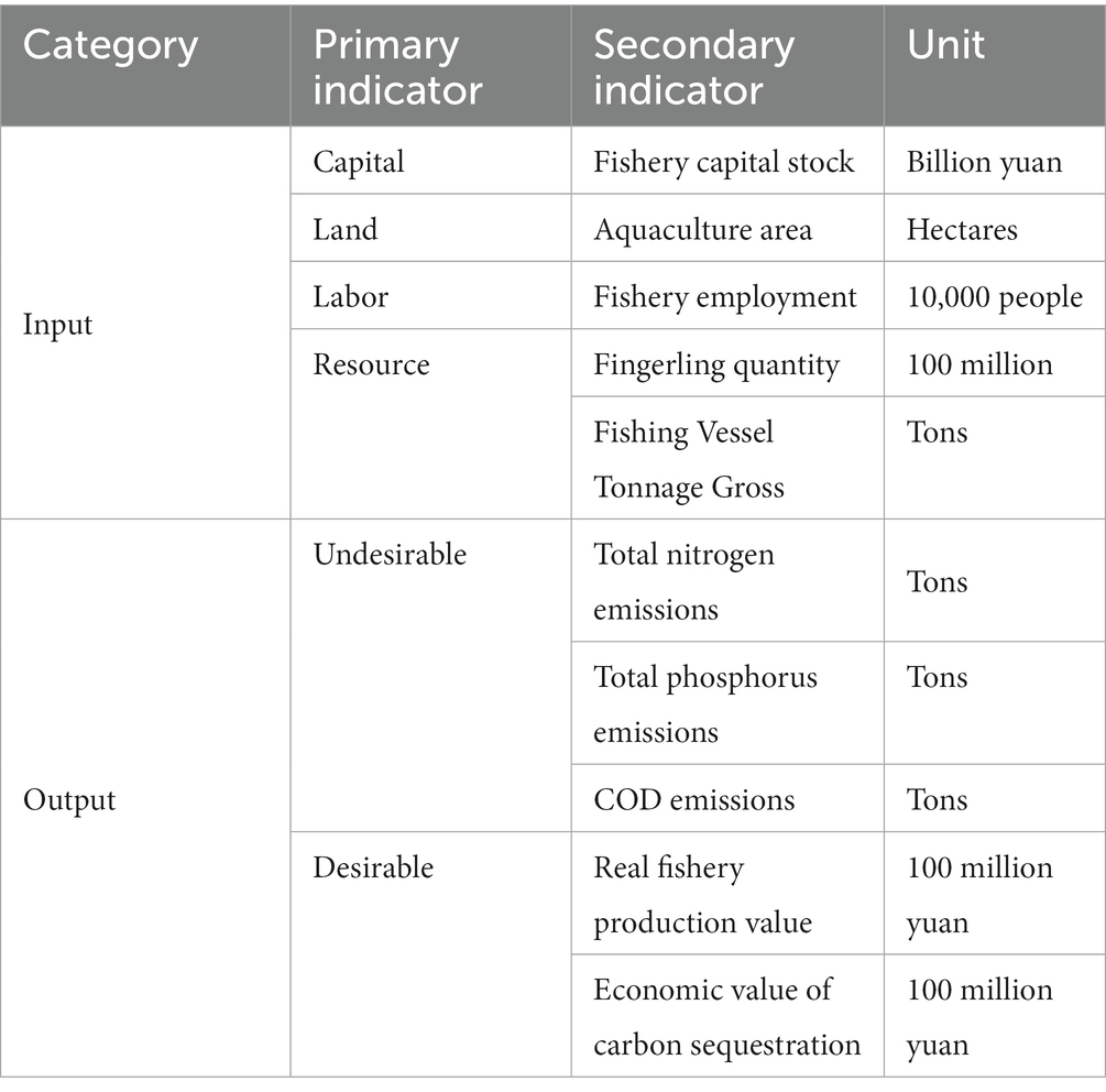
Table 1. The indicators used in the measurement of fisheries GTFP growth.

2.3.2. Indicators used in the analysis of driving forces

In the analysis of driving forces, the dependent variable is the fishery GTFP growth. It is important to note that the fishery GTFP, derived from the EBM model of non-desired outputs and the GML index, represents the concept of year-on-year growth rate and cannot be directly used as the dependent variable. Following previous studies, the cumulative growth of fishery GTFP is calculated using the initial year of the research sample as the base year, which is used as the dependent variable (Yan et al., 2020; Lee and Lee, 2022). To examine the spatial correlation of fishery GTFP growth and its decomposition components, the corresponding Moran’s I index is calculated, and the results are presented in Table 2. It indicates that most years show a positive Moran’s I index, but only in 2013, 2014, 2015, and 2016 are the results statistically significant. For the fishery efficiency growth, the Moran’s I index is positive and statistically significant in most years, while for the fishery technology growth, the Moran’s I index is positive in most years, but statistically significant only in 2007, 2009, and 2019. These results suggest that fishery efficiency growth exhibits a more significant spatial correlation compared to fishery technology growth. Fisheries efficiency typically involves issues related to fisheries production management, and the diffusion of management knowledge can occur more rapidly through collaboration and exchange among fisheries producers in different provinces. In contrast, fisheries technological advancements involve technical aspects and may involve patent-related issues, resulting in relatively weaker spillover effects. The findings in Table 2 indicate the existence of spatial correlation. Therefore, it is necessary to employ spatial econometric models in the analysis of driving forces.

TABLE 2

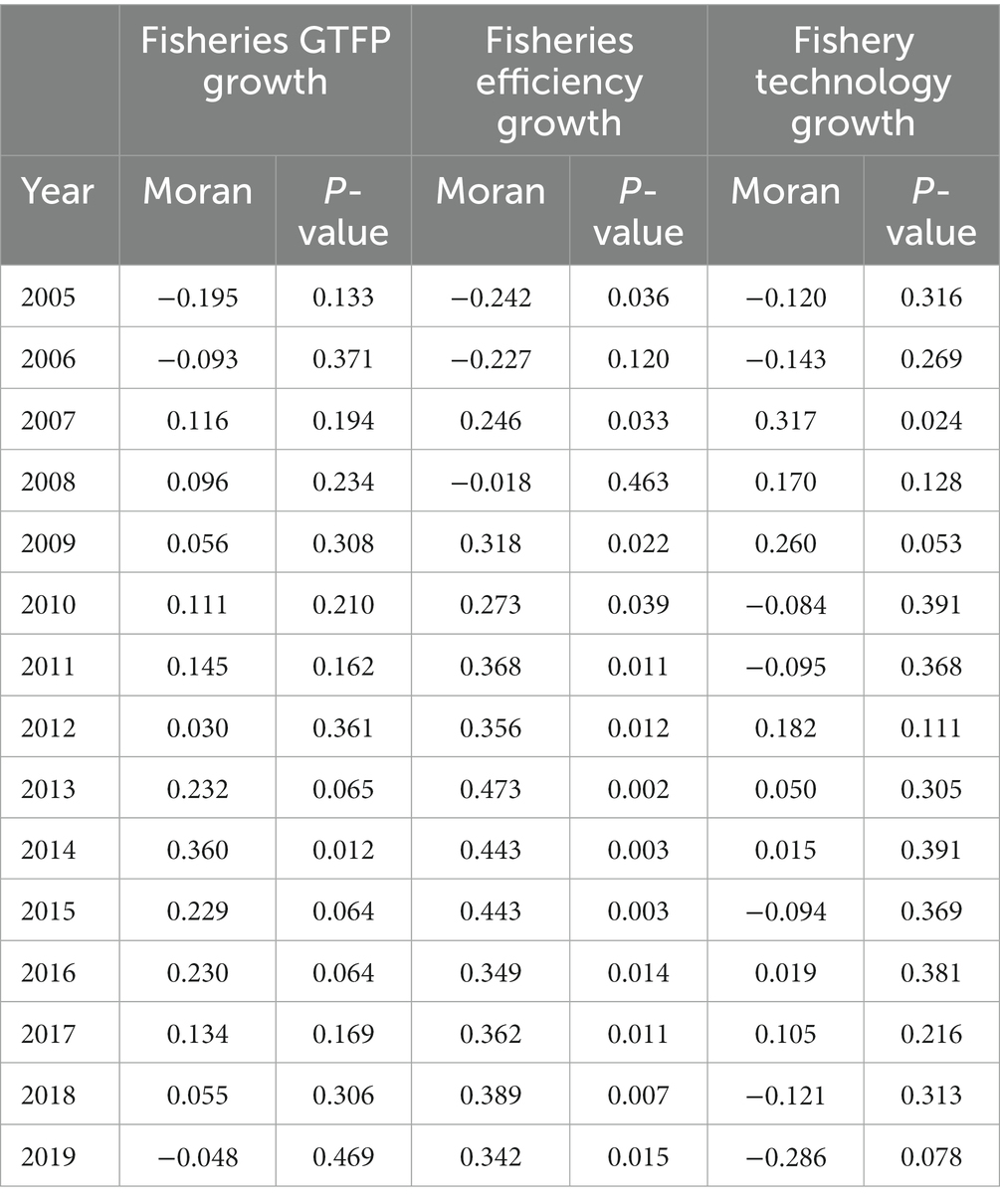
Table 2. Spatial correlation test of fisheries GTFP growth and its decomposed components.

The independent variables are selected based on five dimensions: natural environment, infrastructure, human capital, market size, and government governance. The natural environment is measured by variables such as temperature (temp) and the incidence of fisheries disasters (natdis). Infrastructure is assessed using indicators such as internet penetration rate (internet) and transportation convenience (trans). Human capital is captured through indicators such as the education level of fishermen (aedu) and the provision of fisheries technical training (lnpeop). Market size is represented by trade openness (fishopen) and urbanization rate (urban. Government governance is evaluated by the proportion of environmental governance investment to gross domestic product (envir).

2.3.3. Data source

China’s fisheries GTFP growth is calculated using data from 30 provincial-level administrative region for the period of 2004–2019. The chosen time frame is based on the availability of data, as data prior to 2004 and after 2019 have significant gaps. Provincial-level administrative region such as Tibet, Hong Kong, Macau, and Taiwan were not included in the analysis due to limited data availability.

Data on aquaculture area, fisheries employment, fry quantity, and fishing vessel tonnage are sourced from the “China Fishery Statistical Yearbook” for input indicators. Fisheries capital input calculation utilizes fixed capital formation, fixed asset investment price index, and regional GDP data from the “China Statistical Yearbook.” undesirable output, including total nitrogen, total phosphorus, and COD emissions, are calculated using production data for different fishery species from the “China Fishery Statistical Yearbook,” combined with pollutant emission coefficients from the “Handbook of Pollutant Generation and Discharge Coefficients for Aquaculture in the First National Pollution Source Census.” Desirable output, represented by fishery value-added, is obtained from the “China Fishery Statistical Yearbook,” while the economic value of carbon sequestration is estimated using production data for shellfish and algae from the “China Fishery Statistical Yearbook.”

In the section on driving force analysis, data for calculating provincial average temperature is obtained from the “China Meteorological Science Data Sharing Service Platform.” To derive provincial average temperature, spatial interpolation is applied to convert daily observations from various weather stations into grid-point data, which is then regionally averaged. Fishery disaster area, aquaculture area, fishery technical training attendance, fishery trade, and total fishery output are sourced from the “China Fishery Statistical Yearbook.” Internet penetration rate is obtained from the “Statistical Report on Internet Development in China.” Grade highway is sourced from the “China Transport Statistics Yearbook.” Rural labor force education level is derived from the “China Population and Employment Statistics Yearbook.” Exchange rate from the “China Statistical Yearbook” is used to convert fishery trade volume reported in USD to CNY. Urbanization rate data is sourced from the “China Statistical Yearbook.” Environmental governance investment is obtained from the “China Environmental Statistics Yearbook.”

3. Results

3.1. Measurement of TFP and GTFP growth in China’s fisheries sector

Based on the EBM model and the GML index, this study estimated China’s fishery GTFP growth and its decomposition from 2004 to 2019. The estimation results are presented in Table 3. The results show that the annual average fishery GTFP experienced positive growth in 11 provincial-level administrative regions, including Qinghai, Hubei, Ningxia, Chongqing, Gansu, Fujian, Guizhou, Shaanxi, Beijing, Shanxi, and Jiangsu. Among them, Qinghai had the highest growth rate, reaching 4.7%. Compared to most provinces, Qinghai has a lower level of fishery development, which allows it to have greater growth potential than some other provinces. By learning from more developed provinces in the field of fisheries, Qinghai can access opportunities for rapid growth. Meanwhile, 19 provincial-level administrative regions, including Shanghai, Yunnan, Inner Mongolia, Jilin, Sichuan, Tianjin, Anhui, Shandong, Guangdong, Guangxi, Xinjiang, Jiangxi, Hebei, Henan, Zhejiang, Hainan, Hunan, Liaoning, and Heilongjiang, experienced a decline in annual average fishery GTFP. Among them, Henan had the fastest decline rate, with an average annual decrease of −4.2%. Looking at the decomposition components, efficiency showed positive growth in 10 provincial-level administrative regions, while technology exhibited positive growth in 27 regions. Moreover, in 23 regions, the rate of technological progress was faster than the rate of efficiency improvement. Overall, the growth of fishery GTFP was mainly driven by technological progress.

TABLE 3

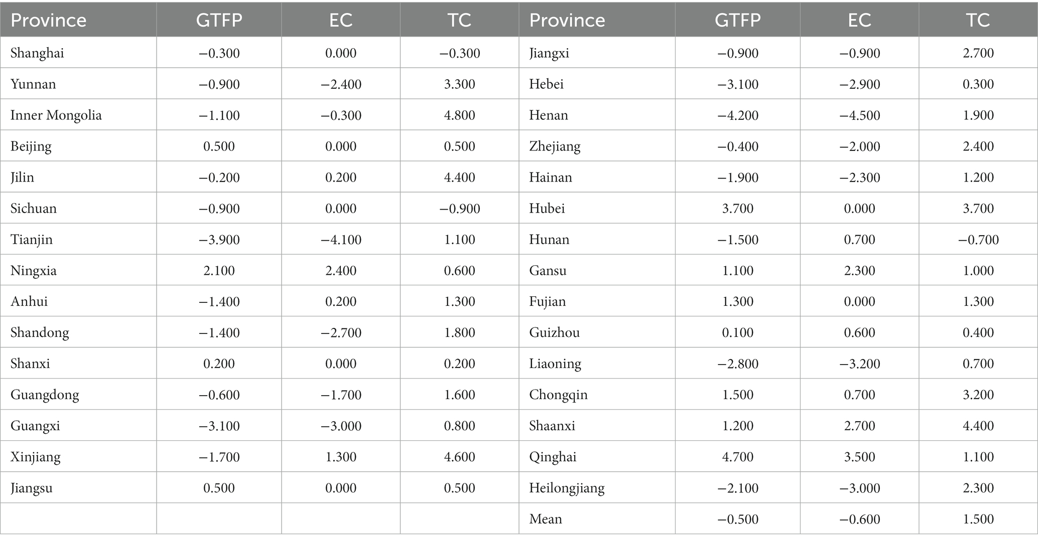
Table 3. Average annual growth rates of fishery GTFP by province, 2004–2019.

In addition, an interesting finding from Table 3 is that coastal provinces such as Shandong, Guangdong, and Zhejiang, known for their developed coastal areas, exhibit negative growth rates in fishery GTFP. These rates are significantly lower than those observed in some less-developed inland provinces. This finding may seem counterintuitive, as coastal provinces typically possess better technological conditions and institutional foundations. Several factors could account for this divergence. The decline in fishery GTFP in coastal provinces can be partially attributed to the substantial scale of fishing and aquaculture operations in these regions. The heightened strain on fishery resources and the environment might impede the overall fishery TFP level, particularly considering the environmental challenges specific to coastal areas. Another contributing factor could be the structural issues in resource allocation. Given their natural advantages as coastal regions, these provinces tend to prioritize marine aquaculture in resource allocation decisions. Consequently, the proliferation of marine ranches or blue grain storages, which require significant financial support, may inadvertently lead to a crowding-out effect on the development of freshwater aquaculture in coastal provinces. This phenomenon, in turn, might result in a relatively slower growth rate of freshwater aquaculture and ultimately impede the overall growth of fishery GTFP in these regions.

To further support this analysis, Table 4 provides additional insights by presenting the average annual growth rates of freshwater aquaculture and marine aquaculture GTFP for the 11 coastal provincial-level administrative regions. Averagely, the growth rate of marine aquaculture GTFP in coastal provinces from 2004 to 2019 was 9%, surpassing the average growth rate of 1.6% observed in freshwater aquaculture. These findings underscore the substantial divergence between the growth rates of marine and freshwater aquaculture GTFP.

TABLE 4

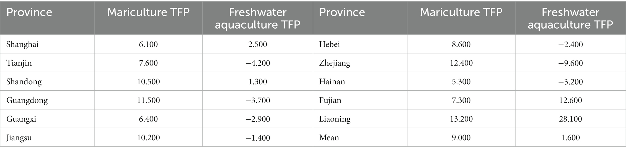
Table 4. Average growth rate of fishery GTFP in coastal provinces from 2004 to 2019.

Examining the provinces individually, except for Fujian and Liaoning, the growth rate of marine aquaculture TFP is higher than that of freshwater aquaculture TFP in all provinces. Combining the information from Tables 3, 4, it can be concluded that the lower growth rate of fishery TFP in coastal provinces is primarily due to the relatively lower growth rate of freshwater aquaculture TFP. This may reflect the crowding out effect of the rapid development of marine aquaculture on the development of freshwater aquaculture in coastal provinces, highlighting the contradiction in resource allocation between marine and freshwater aquaculture.

To compare the differences between fishery GTFP growth and TFP growth, Table 5 presents the estimation results of fishery TFP growth. By comparing these results with those in Table 3, it is evident that, on average, fishery GTFP has a growth rate of −0.5%, while TFP has a growth rate of 0.8%, indicating a difference of 1.3 percentage points. Therefore, disregarding the negative environmental externalities associated with fishery production can lead to an overestimation of fishery TFP growth. Similar conclusions have been drawn in studies from the agricultural sector (Pan and Ying, 2013), highlighting the tendency to overestimate TFP when environmental factors are not considered. Furthermore, substantial variations in efficiency are observed. When considering the negative environmental externalities, the growth rate stands at −0.6%, in contrast to the growth rate of 1.3% without such considerations, signifying a significant discrepancy of 1.9 percentage points. A noteworthy distinction arises from the fact that the fishery technological progress displays negative growth when environmental externalities are overlooked, while it exhibits positive growth when accounting for these factors. This phenomenon may be attributed to the increasing emphasis on environmentally friendly-oriented technological advancements within China’s marine aquaculture sector during the examined time frame (Ren and Zeng, 2021).

TABLE 5

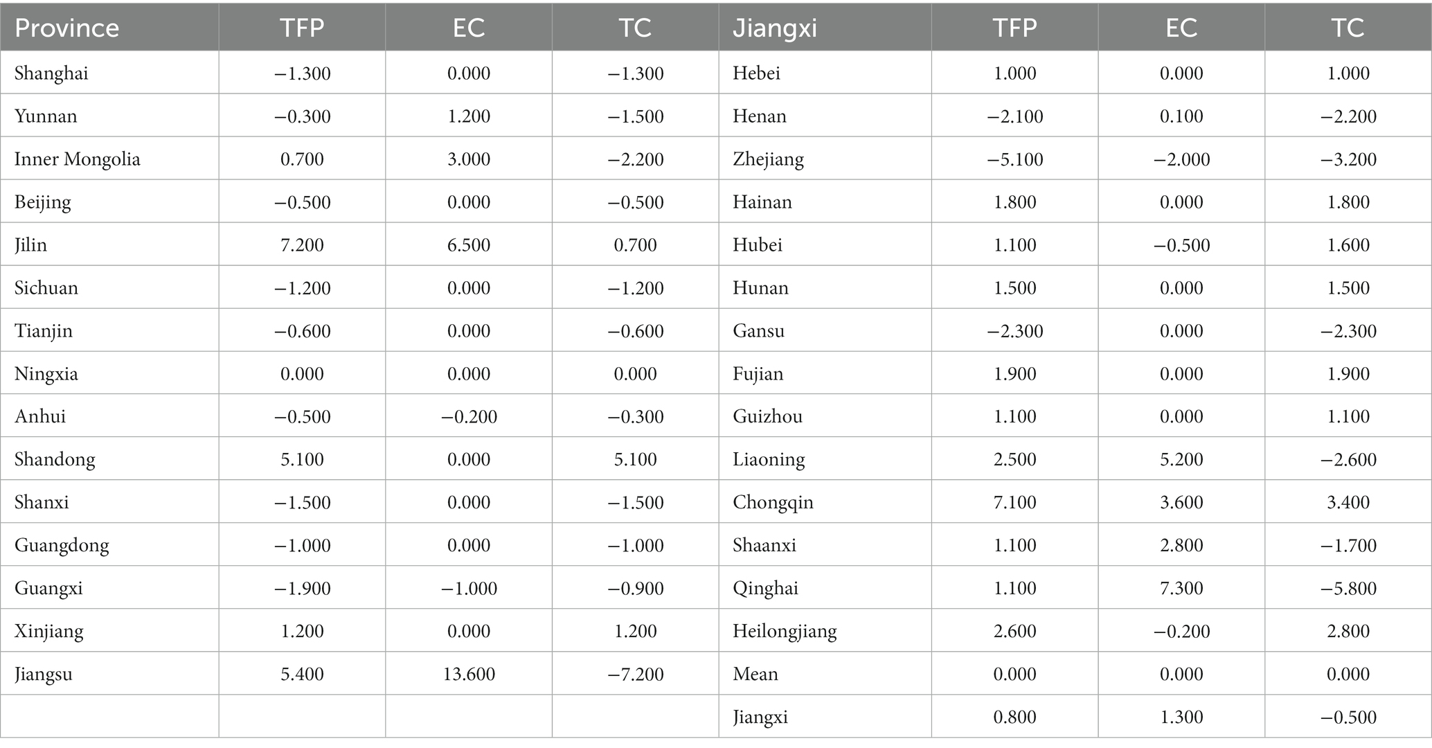
Table 5. Average annual growth rates of fishery TFP by province, 2004–2019.

3.2. Comparison of TFP and GTFP growth trend in China’s fisheries sector

Figure 1 presents the trends in fisheries TFP and GTFP. It also depicts the growth trend of fisheries output in constant prices (using 2004 as the base year). It is worth noting that the TFP (GTFP) calculated based on the GML index represents the relative change from the previous period and does not directly reflect the absolute change. To address this limitation, this study follows the approach suggested by previous studies (Li and Tao, 2012; Liu et al., 2022), where the TFP (GTFP) in 2004 is set as the reference point (equal to 1), and subsequent TFP (GTFP) values are computed by multiplying the TFP (GTFP) growth rate in each year by the corresponding GML index. This methodology is also applied to measure the growth of fisheries output to ensure comparability.

FIGURE 1

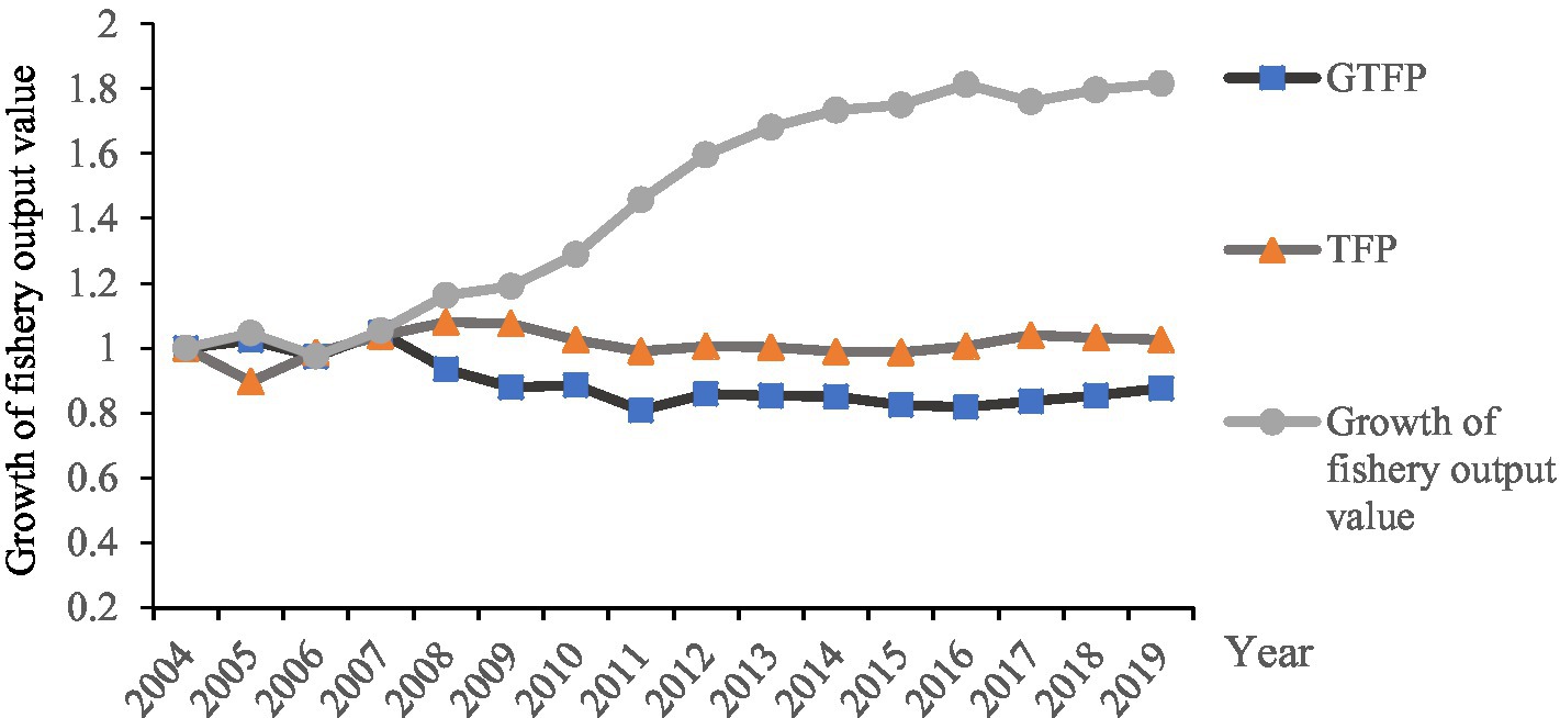
Figure 1. The trends of fishery TFP and GTFP growth.

It can be found that the fisheries sector’s output exhibits an overall upward trend. However, both TFP and GTFP show a slight decline, indicating that the growth in fisheries is driven by intensive factor inputs rather than contributions from TFP. In China’s aquaculture industry, the majority of fish farmers operate on a small scale, resulting in a limited degree of scale efficiency. Their strategy for achieving higher output often involves increasing input factors such as feed and fingerlings per unit area, while investments in technology and management practices remain inadequate. In the fishing industry, increased inputs such as fishing vessels and labor are often utilized to enhance catch volumes, ultimately depleting fishery resources. The East China Sea has even experienced a situation where there are “no fish to catch,” reflecting the extensive nature of fishing practices.

Additionally, an interesting phenomenon is observed. Before 2007, fisheries output growth was similar to TFP growth. However, a significant divergence occurred after 2007, with fisheries output continuing to increase while TFP experienced a slight decline. This phenomenon suggests that the contribution of input factors to fisheries growth is expanding, while the contribution of TFP is diminishing. This may be related to China’s previous extensive economic development pattern. Following the global financial crisis in 2008, the Chinese government initiated large-scale investments to mitigate the crisis, contributing to the extensive nature of China’s economic development to some extent. Additionally, the economic growth pressure resulting from financial crises may lead to a relaxation of environmental regulatory.

3.3. Spatial evolution of GTFP growth in China’s fisheries sector

Figure 2 presents the spatial distribution of the GTFP growth in the Chinese fisheries sector for the years 2004–2005 and 2018–2019. According to Figure 2A, during the period of 2004–2005, the provincial-level administrative region with positive growth in fisheries GTFP are Xinjiang, Qinghai, Inner Mongolia, Jilin, Yunnan, Hunan, Anhui, Liaoning, Shandong, Shaanxi, Chongqing, Guizhou, Hubei, Jiangxi, Shanghai, Zhejiang, and Guangdong, totaling 17 provincial-level administrative regions. Among them, Xinjiang, Qinghai, Shaanxi, Chongqing, Guizhou, Hubei, Liaoning, Jilin, Shandong, Jiangxi, Guangdong, Zhejiang, and Shanghai exhibited the fastest growth, belonging to the first tier. However, 13 provinces and cities including Heilongjiang, Gansu, Sichuan, Ningxia, Shanxi, Henan, Hebei, Beijing, Tianjin, Jiangsu, Guangxi, Hainan, and Fujian experienced a negative growth in GTFP in their fisheries sector.

FIGURE 2

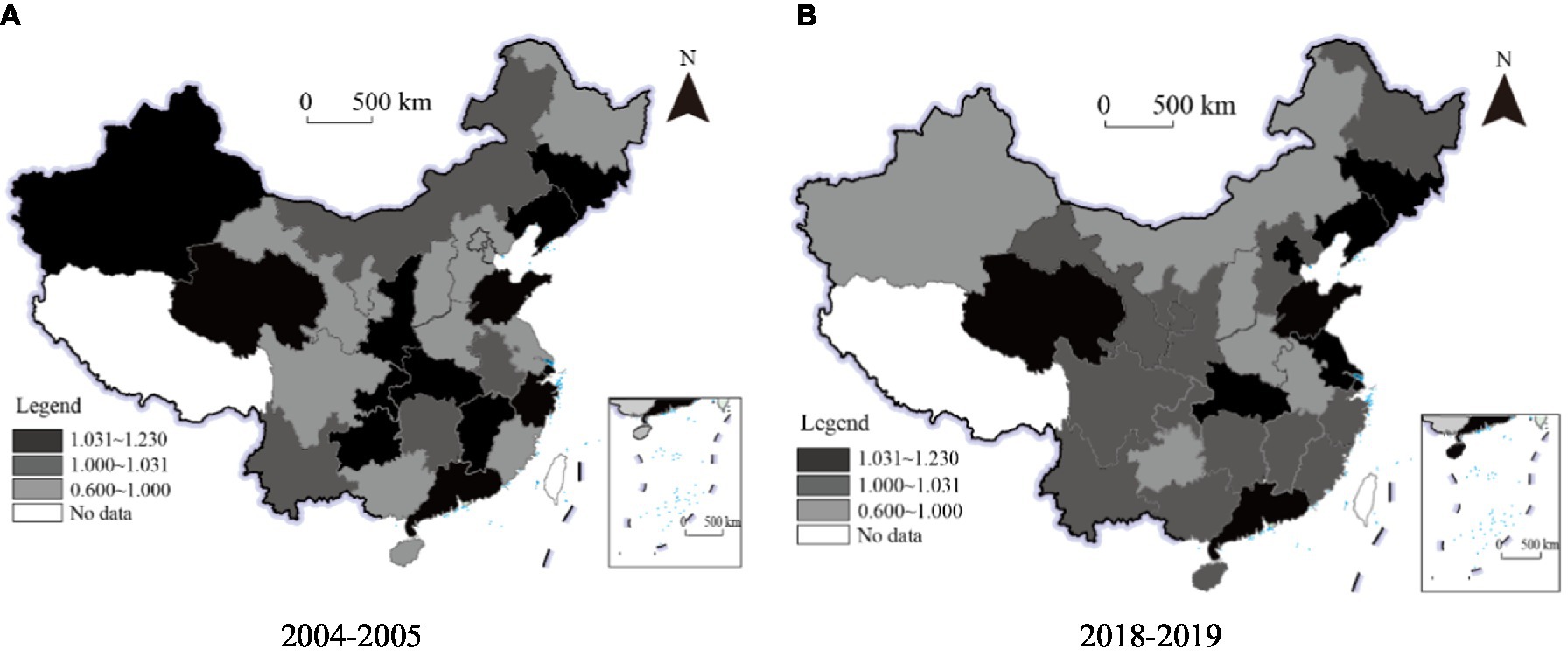
Figure 2. Spatial distribution and evolution of GTFP growth in China’s fisheries industry. China’s administrative system, Beijing, Shanghai, Tianjin, and Chongqing are considered municipalities directly under the central government and are at the same administrative level as provincial-level regions. Therefore, when referring to “cities” in the text, we are specifically talking about these four direct-administered municipalities.

According to Figure 2B, by 2019, there have been significant changes in the spatial distribution pattern of GTFP in China’s fisheries sector. In terms of quantity, compared to the period of 2004–2005, the number of provincial-level administrative regions with positive growth rates in GTFP increased significantly during 2018–2019, with a total of 24 regions experiencing positive growth. However, the number of regions belonging to the first tier in terms of growth decreased from 13 to 10.

Furthermore, examining the evolution of spatial distribution, it can be found that during the 2004–2005 period, the provincial-level administrative regions with the fastest growth rates were mainly located in the central and western regions. However, by 2018–2019, the provincial-level administrative regions with the fastest growth rates were primarily concentrated in the eastern coastal areas, with 8 out of the top 10 fastest-growing situated in the eastern region. Since China’s accession to the WTO in 2001, the pace of opening up to the outside world has accelerated. As a forefront of openness, the eastern region has gained unprecedented development opportunities. The export volume of aquatic products has also increased significantly. However, the development of the fisheries sector has been relatively extensive, and the increase in export volume may have further solidified this development mode. Consequently, the growth of GTFP in certain provinces in the eastern region were relatively lower during the 2004–2005 period. However, since the new government took office in 2013, there has been a shift toward advocating high-quality development in the fisheries sector at the policy level. On the practical front, there have been continuous efforts to promote technological innovation and management practices. Leveraging better technological and industrial foundations, the eastern region has been at the forefront among all provinces and cities, leading to a rapid growth in GTFP in the fisheries sector.

3.4. Drivers of GTFP growth in China’s fisheries sector

3.4.1. Estimation results of spatial econometric models

In this section, the initial model used is the SDM. The Hausman test is employed to determine whether the fixed effects should be included. The p-value based on the Hausman test, as shown in Table 6, is 0.000, rejecting the use of the Random Effects (RE) model. The Likelihood Ratio test is conducted to choose between individual fixed effects, time fixed effects, and the combination of both. The LR test results indicate that the p-values for all the options are 0.000, rejecting the use of only individual fixed effects or time fixed effects. Thus, the appropriate choice is the two-way fixed effects that includes both individual and time fixed effects. The three traditional spatial econometric model specifications are SDM, SAR, and SEM. For the same research question, these models may yield different estimation results. Therefore, before conducting model estimation, it is necessary to determine the specific model form. This study follows the testing strategy proposed by LeSage (2008) as well as Elhorst (2010). The SDM model is initially tested to examine whether it can degenerate into the SAR and SEM models. According to the results of the Wald test and LR test presented in Table 3, it is concluded that the SDM model cannot degenerate into the SEM and SAR models. Hence, the appropriate model choice is the SDM model. Considering all the testing results, this study adopts the SDM with two-way fixed effects. All subsequent empirical analyzes in this study will be based on this model.

TABLE 6

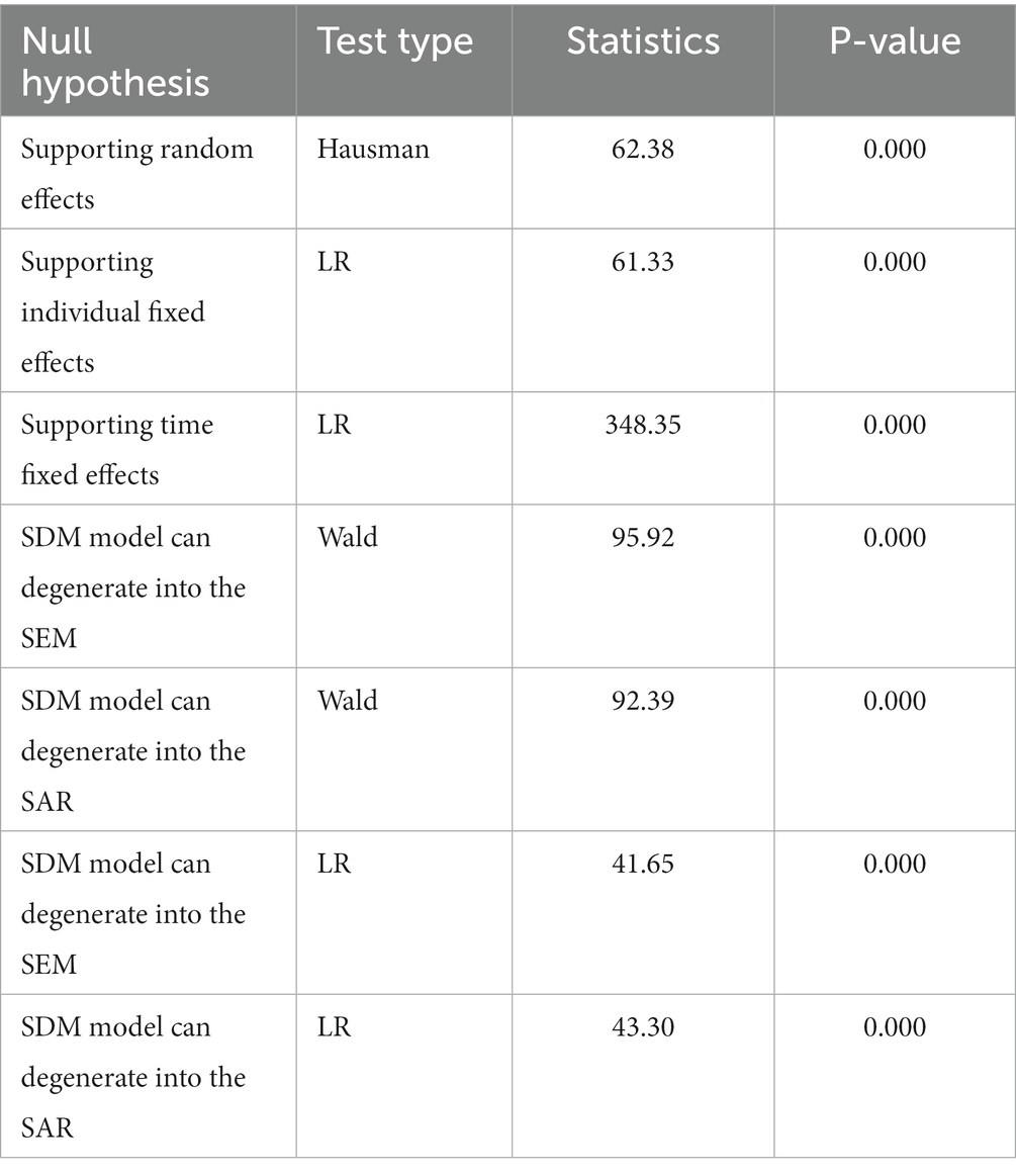
Table 6. Model test results.

Table 7 presents the estimation results of the model, columns (1) show that the spatial autoregressive coefficients ρ are all significantly positive. This suggests that provinces with similar levels of economic development in terms of their fisheries sector tend to mutually enhance their TFP, demonstrating a beneficial spatial interactive pattern.

TABLE 7

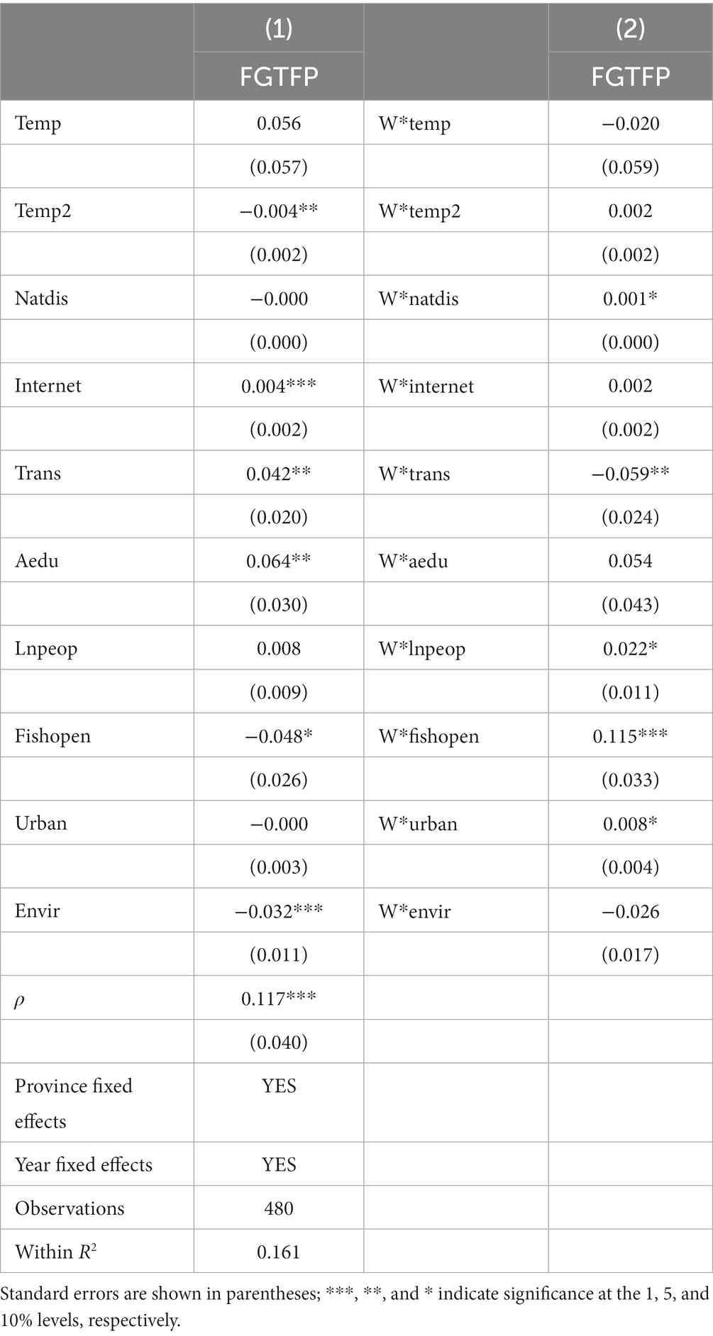
Table 7. Estimated results of the SDM.

Columns (1) to (2), present the estimated results of the effects of natural environment, infrastructure, human capital, macroeconomic conditions, and government governance factors, as well as their spatial lag terms, on fisheries GTFP. Considering that the effect of rising temperature on fisheries GTFP may not be linear, the quadratic term of temperature is included in the model. The results show that the coefficient of the quadratic term of temperature is negative and statistically significant, indicating a “inverted U-shaped” relationship between temperature and fisheries GTFP. This suggests that excessively high temperatures are detrimental to the improvement of GTFP. Internet penetration rate and transportation convenience both show significant positive correlations with fisheries GTFP. On one hand, internet usage helps fisheries producers access market information, management information, innovative knowledge, and fisheries technology, thereby improving the productivity of fisheries units. On the other hand, the widespread use of the internet enables fisheries producers to reduce financing costs, influencing fisheries production. Additionally, Ankrah Twumasi et al. (2021) mentioned another positive mechanism of internet usage influencing fisheries GTFP, which is the income effect brought by non-agricultural work that can improve productivity. The increase in non-agricultural income promotes agricultural household income growth, allowing agricultural producers to have more funds to invest in better machinery, equipment, higher-quality feed, or fertilizers, thereby stimulating productivity improvement (Ma et al., 2018).

Regarding human capital, the average education level of rural labor and fisheries technical training are positively correlated with fisheries GTFP, but only the average education level shows statistical significance based on significance tests. According to Wang et al. (2020), there are issues such as insufficient funds, outdated personnel structure, and inefficient management system in the promotion of aquaculture technology in China. This could be an important reason why fisheries technical training has not fully realized its potential. The level of trade openness has a negative correlation with fisheries GTFP, which is contrary to expectations. The potential reason for this is that the increase in trade openness not only expands the market size faced by fisheries producers but also increases the risks and uncertainties they face. The increase in uncertainty associated with trade openness outweighs the benefits it brings to GTFP, resulting in an inhibitory effect. Additionally, the negative impact may be related to the disproportionate increase in input costs such as aquaculture feed, labor, and land, and the price increase of exported fisheries products. The rise in input costs exceeds the increase in output prices, resulting in decreased output per unit of input and lowered fisheries GTFP. Another unexpected result is the estimated effect of environmental governance investment intensity. The result shows that the increase in environmental pollution control investment intensity has an inhibitory effect on fisheries TFP. This may be because environmental pollution control investment partly reflects government environmental regulations. According to existing studies (Ryan, 2012; He et al., 2020), in the short term, environmental regulations force producers to reduce pollution emissions, but they also increase the cost expenditure for producers, which hinder the improvement of GTFP.

The spatial lag coefficients for fisheries disaster rate, fisheries technical training person-times, fisheries trade openness, and urbanization rate are all positive and statistically significant. This indicates that an increase in these variables in one province has a positive spatial spillover effect on the fisheries GTFP of its economically similar provinces. The spatial lag coefficient for transportation convenience is negative and statistically significant, suggesting an improvement in transportation convenience in one province has a negative spatial spillover effect on the fisheries GTFP of its economically similar provinces.

3.4.2. Decomposition of spatial effects

Despite the estimation results of the SDM provided in Table 7, which reflect the directions of the effects of natural environment, infrastructure, human capital, market size, and government governance on fishery GTFP, the point estimates of the coefficients do not capture the magnitude of the marginal effects of each factor on fishery GTFP. Therefore, following the approach presented by Lesage and Pace (2010), the effect of the five categories of factors on fishery GTFP is decomposed into direct effect, indirect effect, and total effect. The direct effect refers to the changes in fishery GTFP within a province caused by itself independent variables, including the spatial feedback effect on fishery GTFP. The indirect effect refers to the effect of the independent variables of a province on fishery GTFP in provinces with similar levels of economic development. The total effect is the sum of the direct and indirect effect. The decomposition is presented in Table 8.

TABLE 8

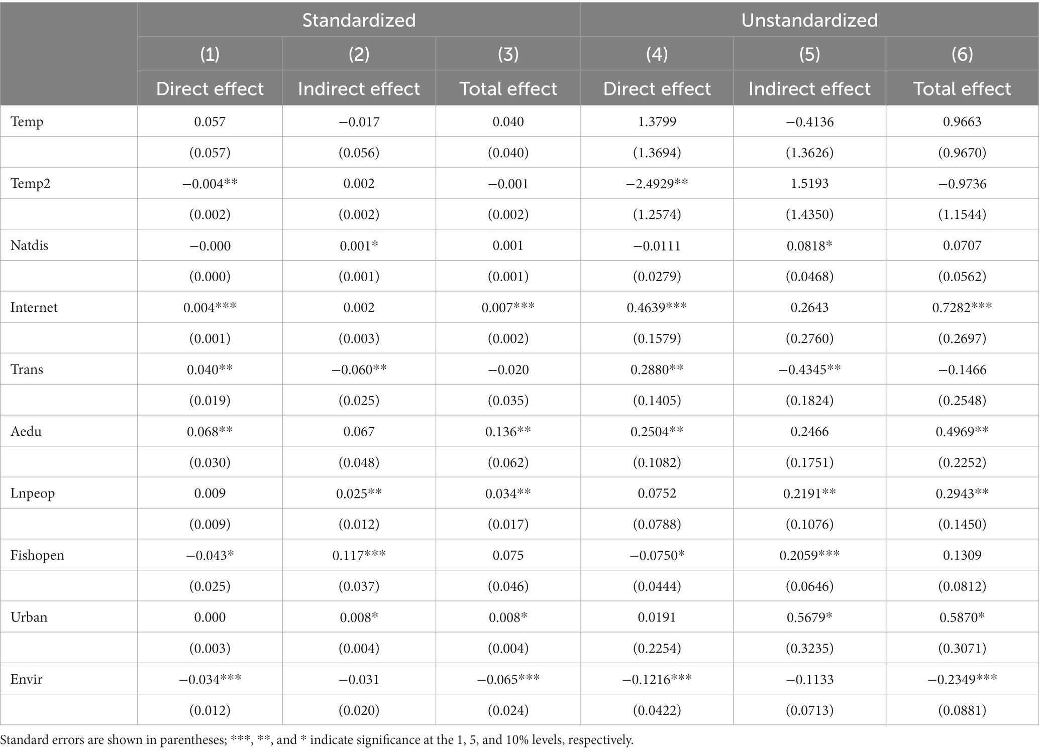
Table 8. The decomposition of spatial effect.

The results of the direct effect in column (1) indicate that the estimated coefficients and significance of the quadratic term for temperature do not exhibit significant changes compared to Table 7. The estimated coefficient and statistical significance of internet penetration rate also remain unchanged. This result suggests that for every one-percentage-point increase in internet penetration rate, fishery GTFP will increase by 0.4%. The estimated coefficient for transportation convenience is 0.040, and it is statistically significant. This implies that for every one-percentage-point increase in the ratio of paved road mileage to land area, fishery GTFP will increase by approximately 0.04%. An increase of 1 year in the average years of education for rural residents will lead to a 6.8% increase in fishery GTFP. For every one-percentage-point increase in the ratio of fishery import and export trade to the total value of fishery production, fishery GTFP will decrease by approximately 0.04%. An increase of one percentage point in the proportion of environmental pollution control investment to GDP will result in a 3.4% decrease in fishery GTFP.

For indirect effect, for every one-percentage-point increase in the average fishery disaster rate of provinces with similar levels of economic development to the province being analyzed, the fishery GTFP of the province being analyzed will increase by approximately 0.1%. For every one-percentage-point increase in the ratio of paved road mileage to land area in provinces with similar levels of economic development to the province being analyzed, the fishery GTFP of the province being analyzed will decrease by approximately 0.06%. For every one-percentage-point increase in the number of technical training sessions for fishermen in provinces with similar levels of economic development to the province being analyzed, the fishery TFP of the province being analyzed will increase by approximately 0.03%. For every one-percentage-point increase in the ratio of import and export trade to the total value of fishery production in provinces with similar levels of economic development to the province being analyzed, the fishery GTFP of the province being analyzed will increase by approximately 0.12%. For every one-percentage-point increase in the urbanization rate in provinces with similar levels of economic development to the province being analyzed, the fishery GTFP of the province being analyzed will increase by approximately 0.8%.

Due to the different scales of the original variables, it is not possible to directly compare the estimated coefficients of the variables in columns (1) to (3) of Table 8. To determine which factor among the five factors of natural environment, infrastructure, human capital, market size, and government governance has the greatest promoting effect on fishery GTFP, all variables are standardized to unify the scales, and the model is re-estimated based on the standardized variables. The results are shown in columns (4) to (6) of Table 8. In column (4), the standardized coefficients of internet penetration rate and transportation convenience are the largest among all variables. Therefore, infrastructure has the largest positive direct effect on China’s fishery GTFP, followed by human capital. Specifically, for every one-standard-deviation increase in internet penetration rate and transportation convenience, the growth rate of fishery GTFP in a province will increase by approximately 0.46 standard deviations and 0.29 standard deviations, respectively. In column (5), the standardized results show that the urbanization rate has the largest positive indirect effect on China’s fishery GTFP, followed by the number of technical training sessions for fishermen and the degree of fishery trade openness. Therefore, in combination, market size has the largest positive indirect effect on China’s fishery GTFP. For every one-standard-deviation increase in the urbanization rate, the number of technical training sessions for fishermen, and the degree of fishery trade openness in a province, the growth rate of fishery GTFP in provinces with similar levels of economic development to this province will increase by approximately 0.57, 0.22, and 0.21 standard deviations, respectively.

4. Conclusions and policy implications

Over the years, the inclusion of negative environmental externalities resulting from aquaculture pollution has posed a challenge in assessing fishery TFP growth at the provincial level in China. This study bridges this gap by estimating the negative environmental externalities associated with aquaculture, utilizing pollutant discharge coefficients from the “Handbook of Pollutant Generation and Discharge Coefficients for Aquaculture in the First National Pollution Source Census,” and aquaculture production data from the “China Fishery Statistical Yearbook.” By amalgamating the fishery capture and aquaculture sectors and integrating the estimations of aquaculture pollution emissions, this study endeavors to measure the GTFP growth of the entire fishery sector while meticulously examining the driving forces behind it.

Our study reveals that disregarding the environmental cost entailed by fishery production activities leads to an overestimation of fishery TFP growth. In comparison to GTFP growth that consider these costs, the growth rate of fishery TFP is inflated by 1.3% when such considerations are disregarded. In terms of its decomposition, the growth of fishery efficiency is overestimated by 0.7%, while fishery technological growth is underestimated by 1% in the absence of accounting for environmental costs. The expansion of fishery output primarily stems from augmented input factors rather than the TFP growth, indicative of an extensive pattern. Nonetheless, considering the progressively decelerating pace of fishery output growth, the contribution of increased input factors is gradually waning. Examining spatial distribution and evolution, we observe that in 2005, provinces and municipalities boasting the swiftest growth rates in GTFP were predominantly situated in China’s central and western regions. Among the 12 provinces with the highest growth rates, 7 were concentrated in these areas. By 2019, the provinces and municipalities leading in growth rates were predominantly found in the eastern region, with 8 out of the top 10 provinces located there.

From the analysis of driving forces, provinces with similar levels of economic development in terms of their fisheries sector tend to mutually enhance their GTFP growth, demonstrating a beneficial spatial interactive pattern. The enhancement of fishery GTFP in a specific province can be facilitated by the improvement of factors such as internet penetration rate, transportation convenience, and rural residents’ education level. Moreover, the fishery disaster rate, fisherman training, fishery trade openness, and urbanization rate in a province exhibit positive spatial spillover effects on the fishery GTFP growth of provinces with similar levels of economic development. When comparing the direct and indirect effects of these driving factors, it becomes apparent that infrastructure factors, including internet penetration rate and transportation convenience, exert the most significant direct influence on fishery GTFP growth. Market size factors, including trade openness and urbanization rate, on the other hand, exhibit the largest indirect effects on fishery GTFP growth.

The enhancement of GTFP in the fishery sector holds significant implications for achieving high-quality economic development in fisheries. Our study offers valuable policy insights to guide the advancement of China’s fishery sector. Firstly, while prioritizing economic gains, it is imperative to ensure a balanced consideration of environmental benefits. This entails intensifying efforts to regulate pollution emissions arising from aquaculture activities and implementing stringent controls to prevent overfishing, thus safeguarding fishery resources. Secondly, the government should amplify its investments in foundational infrastructure, such as internet connectivity and road networks. This strategic approach aims to reduce information exchange costs and enhance logistical efficiency within the fishery sector. Thirdly, fostering regional market integration and bolstering inter-regional collaboration are pivotal. By promoting constructive interactions among different regions, we can stimulate the elevation of fishery GTFP and propel sustainable development.

There are still some areas that need further improvement in this study. Due to the difficulty in obtaining data on fishery resource stocks, this study directly uses the tonnage of fishing vessels as a measure of the pressure exerted by fishery production on fishery resources. However, this indicator may not be entirely accurate. For example, under different fishery resource stocks, the same tonnage of fishing vessels may exert different pressures on fishery resources. If we can collect data on fishery resource stocks in the future, it will enable us to estimate China’s fishery GTFP more accurately and providing stronger support for the formulation of more effective fishery management and policies.

Data availability statement

The raw data supporting the conclusions of this article will be made available by the authors, without undue reservation.

Author contributions

WS: Conceptualization, Methodology, Writing – original draft, Writing – review & editing. HG: Supervision, Writing – review & editing, Data curation, Funding acquisition, Software. JB: Visualization, Data collection.

Funding

The author(s) declare financial support was received for the research, authorship, and/or publication of this article. This research was supported by Zhejiang Province Philosophy and Social Science Planning Project (23NDJC255YB).

Conflict of interest

The authors declare that the research was conducted in the absence of any commercial or financial relationships that could be construed as a potential conflict of interest.

Publisher’s note

All claims expressed in this article are solely those of the authors and do not necessarily represent those of their affiliated organizations, or those of the publisher, the editors and the reviewers. Any product that may be evaluated in this article, or claim that may be made by its manufacturer, is not guaranteed or endorsed by the publisher.

References

Álvarez, A., Couce, L., and Trujillo, L. (2020). Does specialization affect the efficiency of small-scale fishing boats? Mar. Policy 113:103796. doi: 10.1016/j.marpol.2019.103796

CrossRef Full Text | Google Scholar

Ankrah Twumasi, M., Jiang, Y., Zhou, X., Addai, B., Darfor, K. N., Akaba, S., et al. (2021). Increasing Ghanaian fish farms’ productivity: does the use of the internet matter? Mar. Policy 125:104385. doi: 10.1016/j.marpol.2020.104385

CrossRef Full Text | Google Scholar

Aponte, F. R. (2020). Firm dispersion and total factor productivity: are Norwegian salmon producers less efficient over time? Aquac. Econ. Manage. 24, 161–180. doi: 10.1080/13657305.2019.1677803

CrossRef Full Text | Google Scholar

Asche, F., Guttormsen, A. G., and Nielsen, R. (2013). Future challenges for the maturing Norwegian salmon aquaculture industry: an analysis of total factor productivity change from 1996 to 2008. Aquaculture 396-399, 43–50. doi: 10.1016/j.aquaculture.2013.02.015

CrossRef Full Text | Google Scholar

Chang, Y.-C., Zhang, X., and Khan, M. I. (2022). The impact of the COVID-19 on China's fisheries sector and its countermeasures. Ocean Coastal Manage. 216:105975. doi: 10.1016/j.ocecoaman.2021.105975

PubMed Abstract | CrossRef Full Text | Google Scholar

Dey, M. M., Paraguas, F. J., Kambewa, P., and Pemsl, D. E. (2010). The impact of integrated aquaculture–agriculture on small-scale farms in southern Malawi. Agric. Econ. 41, 67–79. doi: 10.1111/j.1574-0862.2009.00426.x

CrossRef Full Text | Google Scholar

Elhorst, J. P. (2010). Applied spatial econometrics: raising the bar. Spat. Econ. Anal. 5, 9–28. doi: 10.1080/17421770903541772

CrossRef Full Text | Google Scholar

Guo, H., and Liu, X. (2021). Spatial and temporal differentiation and convergence of china's agricultural green total factor productivity. J. Quant. Technol. Econ. 38, 65–84. doi: 10.13653/j.cnki.jqte.2021.10.004

CrossRef Full Text | Google Scholar

He, G., Wang, S., and Zhang, B. (2020). Watering down environmental regulation in China. Q. J. Econ. 135, 2135–2185. doi: 10.1093/qje/qjaa024

CrossRef Full Text | Google Scholar

Holland, D., Gudmundsson, E., and Gates, J. (1999). Do fishing vessel buyback programs work: a survey of the evidence. Mar. Policy 23, 47–69. doi: 10.1016/S0308-597X(98)00016-5

CrossRef Full Text | Google Scholar

Holland, D. S., Steiner, E., and Warlick, A. (2017). Can vessel buybacks pay off: an evaluation of an industry funded fishing vessel buyback. Mar. Policy 82, 8–15. doi: 10.1016/j.marpol.2017.05.002

CrossRef Full Text | Google Scholar

Iliyasu, A., Mohamed, Z. A., and Terano, R. (2016). Comparative analysis of technical efficiency for different production culture systems and species of freshwater aquaculture in peninsular Malaysia. Aquac. Rep. 3, 51–57. doi: 10.1016/j.aqrep.2015.12.001

CrossRef Full Text | Google Scholar

Jin, D., Thunberg, E., Kite-Powell, H., and Blake, K. (2002). Total factor productivity change in the New England groundfish fishery: 1964–1993. J. Environ. Econ. Manag. 44, 540–556. doi: 10.1006/jeem.2001.1213

CrossRef Full Text | Google Scholar

Kareem, R. O., Aromolaran, A. B., and Dipeolu, A. O. (2009). Economic efficiency of fish farming in Ogun state, Nigeria. Aquac. Econ. Manage. 13, 39–52. doi: 10.1080/13657300802679145

CrossRef Full Text | Google Scholar

Le, C.-Y., Feng, J.-C., Sun, L., Yuan, W., Wu, G., Zhang, S., et al. (2023). Co-benefits of carbon sink and low carbon food supply via shellfish and algae farming in China from 2003 to 2020. J. Clean. Prod. 414:137436. doi: 10.1016/j.jclepro.2023.137436

CrossRef Full Text | Google Scholar

Lee, C.-C., and Lee, C.-C. (2022). How does green finance affect green total factor productivity? Evidence from China. Energy Econ. 07:105863. doi: 10.1016/j.eneco.2022.105863

CrossRef Full Text | Google Scholar

LeSage, J. P. (2008). An introduction to spatial econometrics. Rev. Econ. Ind. 123, 19–44. doi: 10.4000/rei.3887

CrossRef Full Text | Google Scholar

Lesage, J., and Pace, R. (2010). Spatial econometric models. Berlin, Heidelberg: Springer.

Google Scholar

Li, G. (2014). The green productivity revolution of agriculture in China fr0m 1978 to 2008. China Econ. Q. 13, 537–558. doi: 10.13821/j.cnki.ceq.2014.02.011

CrossRef Full Text | Google Scholar

Li, C., Feng, W., and Shao, G. (2018). Spatio-temporal difference of total carbon emission efficiency of fishery in China. Econ. Geogr. 38, 179–187. doi: 10.15957/j.cnki.jjdl.2018.05.022

CrossRef Full Text | Google Scholar

Li, L., and Tao, F. (2012). Selection of optimal environmental regulation intensity for chinese manufacturing industry-based on the greenTFP perspective. China Ind. Econ. 30, 70–82. doi: 10.19581/j.cnki.ciejournal.2012.05.006

CrossRef Full Text | Google Scholar

Liu, W., Du, M., and Bai, Y. (2022). Impact of environmental regulations on green total factor productivity. China Popul. Resour. Environ. 32, 95–107.

Google Scholar

Long, L. K., Van Thap, L., Hoai, N. T., and Pham, T. T. T. (2020). Data envelopment analysis for analyzing technical efficiency in aquaculture: the bootstrap methods. Aquac. Econ. Manage. 24, 422–446. doi: 10.1080/13657305.2019.1710876

CrossRef Full Text | Google Scholar

Ma, W., Abdulai, A., and Ma, C. (2018). The effects of off-farm work on fertilizer and pesticide expenditures in China. Rev. Dev. Econ. 22, 573–591. doi: 10.1111/rode.12354

CrossRef Full Text | Google Scholar

McClanahan, T., Allison, E. H., and Cinner, J. E. (2015). Managing fisheries for human and food security. Fish Fish. 16, 78–103. doi: 10.1111/faf.12045

CrossRef Full Text | Google Scholar

Mitra, S., Khan, M. A., and Nielsen, R. (2019). Credit constraints and aquaculture productivity. Aquac. Econ. Manage. 23, 410–427. doi: 10.1080/13657305.2019.1641571

CrossRef Full Text | Google Scholar

Mitra, S., Khan, M. A., Nielsen, R., and Islam, N. (2020). Total factor productivity and technical efficiency differences of aquaculture farmers in Bangladesh: do environmental characteristics matter? J. World Aquacult. Soc. 51, 918–930. doi: 10.1111/jwas.12666

CrossRef Full Text | Google Scholar

Newell, R. G., Sanchirico, J. N., and Kerr, S. (2005). Fishing quota markets. J. Environ. Econ. Manag. 49, 437–462. doi: 10.1016/j.jeem.2004.06.005

CrossRef Full Text | Google Scholar

Nielsen, R., Hoff, A., and Andersen, J. L. (2023). Structural and productivity changes from introducing strong user rights in the Danish demersal fisheries. Mar. Policy 147:105385. doi: 10.1016/j.marpol.2022.105385

CrossRef Full Text | Google Scholar

Oh, D. H. (2010). A global Malmquist-Luenberger productivity index. J. Prod. Anal. 34, 183–197. doi: 10.1007/s11123-010-0178-y

CrossRef Full Text | Google Scholar

Pan, W., Xie, T., Wang, Z., and Ma, L. (2022). Digital economy: an innovation driver for total factor productivity. J. Bus. Res. 139, 303–311. doi: 10.1016/j.jbusres.2021.09.061

CrossRef Full Text | Google Scholar

Pan, D., and Ying, R. (2013). Agricultural total factor productivity growth in China under the binding of resource and environment. Resour. Sci. 35, 1329–1338.

Google Scholar

Pascoe, S., Coglan, L., Punt, A. E., and Dichmont, C. M. (2012). Impacts of vessel capacity reduction programmes on efficiency in fisheries: the case of australia’s multispecies northern prawn fishery. J. Agric. Econ. 63, 425–443. doi: 10.1111/j.1477-9552.2011.00333.x

CrossRef Full Text | Google Scholar

Pascoe, S., and Tingley, D. (2007). “Capacity and technical efficiency estimation in fisheries: parametric and non-parametric techniques” in Handbook of operations research in natural resources. eds. A. Weintraub, C. Romero, T. Bjørndal, R. Epstein, and J. Miranda (Boston, MA: Springer US), 273–294.

Google Scholar

Pincinato, R. B. M., Asche, F., Cojocaru, A. L., Liu, Y., and Roll, K. H. (2021). The impact of transferable fishing quotas on cost, price, and season length. Mar. Resour. Econ. 37, 53–63. doi: 10.1086/716728

CrossRef Full Text | Google Scholar

Pipitone, V., and Colloca, F. (2018). Recent trends in the productivity of the Italian trawl fishery: the importance of the socio-economic context and overexploitation. Mar. Policy 87, 135–140. doi: 10.1016/j.marpol.2017.10.017

CrossRef Full Text | Google Scholar

Ren, W., and Zeng, Q. (2021). Is the green technological progress bias of mariculture suitable for its factor endowment? Empirical results from 10 coastal provinces and cities in China. Mar. Policy 124:104338. doi: 10.1016/j.marpol.2020.104338

CrossRef Full Text | Google Scholar

Ryan, S. P. (2012). The costs of environmental regulation in a concentrated industry. Econometrica 80, 1019–1061. doi: 10.3982/ECTA6750

CrossRef Full Text | Google Scholar

Sanchirico, J. N., Holland, D., Quigley, K., and Fina, M. (2006). Catch-quota balancing in multispecies individual fishing quotas. Mar. Policy 30, 767–785. doi: 10.1016/j.marpol.2006.02.002

CrossRef Full Text | Google Scholar

Sea, M. A., Hillman, J. R., and Thrush, S. F. (2022). The influence of mussel restoration on coastal carbon cycling. Glob. Chang. Biol. 28, 5269–5282. doi: 10.1111/gcb.16287

PubMed Abstract | CrossRef Full Text | Google Scholar

See, K. F., Ibrahim, R. A., and Goh, K. H. (2021). Aquaculture efficiency and productivity: a comprehensive review and bibliometric analysis. Aquaculture 544:736881. doi: 10.1016/j.aquaculture.2021.736881

CrossRef Full Text | Google Scholar

Shao, G., Liu, B., and Li, C. (2019). Evaluation of carbon dioxide capacity and the effects of decomposition and spatio-temporal differentiation of seawater in China's main sea area based on panel data from 9 coastal provinces in China. Acta Ecol. Sin. 39, 2614–2625.

Google Scholar

Shao, Y., Wang, Y., Yuan, Y., and Xie, Y. (2021). A systematic review on antibiotics misuse in livestock and aquaculture and regulation implications in China. Sci. Total Environ. 798:149205. doi: 10.1016/j.scitotenv.2021.149205

CrossRef Full Text | Google Scholar

Solís, D., Agar, J. J., and del Corral, J. (2015). IFQs and total factor productivity changes: the case of the Gulf of Mexico red snapper fishery. Mar. Policy 62, 347–357. doi: 10.1016/j.marpol.2015.06.001

CrossRef Full Text | Google Scholar

Solís, D., del Corral, J., Perruso, L., and Agar, J. J. (2014). Evaluating the impact of individual fishing quotas (IFQs) on the technical efficiency and composition of the US Gulf of Mexico red snapper commercial fishing fleet. Food Policy 46, 74–83. doi: 10.1016/j.foodpol.2014.02.005

CrossRef Full Text | Google Scholar

Solow, R. M. (1957). Technical change and the aggregate production function. Rev. Econ. Stat. 39, 312–320. doi: 10.2307/1926047

CrossRef Full Text | Google Scholar

Squires, D. (1992). Productivity measurement in common property resource industries: an application to the pacific coast trawl fishery. Rand J. Econ. 23, 221–236. doi: 10.2307/2555985

CrossRef Full Text | Google Scholar

Sun, K., Cui, X., Su, Z., and Wang, Y. (2020). Spatio-temporal evolution and influencing factors of the economic value for mariculture carbon sinks in China. Geogr. Res. 39, 2508–2520.

Google Scholar

Sun, K., Ji, J., Li, L., Zhang, C., Liu, J., and Fu, M. (2017). Marine fishery economic efficiency and its spatio- temporal differences based on undesirable outputs in China. Resour. Sci. 39, 2040–2051. doi: 10.18402/resci.2017.11.03

CrossRef Full Text | Google Scholar

Tone, K., and Tsutsui, M. (2010). An epsilon-based measure of efficiency in DEA–a third pole of technical efficiency. Eur. J. Oper. Res. 207, 1554–1563. doi: 10.1016/j.ejor.2010.07.014

CrossRef Full Text | Google Scholar

Van Beveren, I. (2012). Total factor productivity estimation: a practical review. J. Econ. Surv. 26, 98–128. doi: 10.1111/j.1467-6419.2010.00631.x

CrossRef Full Text | Google Scholar

Van Nguyen, Q., Pascoe, S., Coglan, L., and Nghiem, S. (2021). The sensitivity of efficiency scores to input and other choices in stochastic frontier analysis: an empirical investigation. J. Prod. Anal. 55, 31–40. doi: 10.1007/s11123-020-00592-8

CrossRef Full Text | Google Scholar

Van Nguyen, Q., and See, K. F. (2023). Application of the frontier approach in capture fisheries efficiency and productivity studies: a bibliometric analysis. Fish. Res. 263:106676. doi: 10.1016/j.fishres.2023.106676

CrossRef Full Text | Google Scholar

Walden, J. B., Kirkley, J. E., Färe, R., and Logan, P. (2012). Productivity change under an individual transferable quota management system. Am. J. Agric. Econ. 94, 913–928. doi: 10.1093/ajae/aas025

CrossRef Full Text | Google Scholar

Wang, P., Ji, J., and Zhang, Y. (2020). Aquaculture extension system in China: development, challenges, and prospects. Aquac. Rep. 17:100339. doi: 10.1016/j.aqrep.2020.100339

CrossRef Full Text | Google Scholar

Wang, S. L., and Walden, J. B. (2021). Measuring fishery productivity growth in the northeastern United States 2007–2018. Mar. Policy 128:104467. doi: 10.1016/j.marpol.2021.104467

CrossRef Full Text | Google Scholar

Wu, P., Wang, Y., Chiu, Y. H., Li, Y., and Lin, T.-Y. (2019). Production efficiency and geographical location of Chinese coal enterprises - undesirable EBM DEA. Resour. Policy 64:101527. doi: 10.1016/j.resourpol.2019.101527

CrossRef Full Text | Google Scholar

Yan, Z., Zou, B., Du, K., and Li, K. (2020). Do renewable energy technology innovations promote China's green productivity growth? Fresh evidence from partially linear functional-coefficient models. Energy Econ. 90:104842. doi: 10.1016/j.eneco.2020.104842

CrossRef Full Text | Google Scholar

Ye, F., Qin, S., Nisar, N., Zhang, Q., Tong, T., and Wang, L. (2023). Does rural industrial integration improve agricultural productivity? Implications for sustainable food production. Front. Sustain. Food Syst. 7:1024. doi: 10.3389/fsufs.2023.1191024

CrossRef Full Text | Google Scholar

Yu, D., Liu, L., Gao, S., Yuan, S., Shen, Q., and Chen, H. (2022). Impact of carbon trading on agricultural green total factor productivity in China. J. Clean. Prod. 367:132789. doi: 10.1016/j.jclepro.2022.132789

CrossRef Full Text | Google Scholar

Zhang, M., Cheng, Z., and Fan, Y. (2023). Exploring the impact of insect-resistant transgenic cotton application on agriculture total factor productivity under climate change. J. Agrotech. Econ. 42, 17–34.

Google Scholar

Zhang, X., Shan, Z., and Yu, L. (2020). Green efficiency measurement and spatial spillover effect of china's marine carbon sequestration fishery. Chinese Rural Econ. 36, 91–110.

Google Scholar

Zhong, S., Li, A., and Wu, J. (2022). The total factor productivity index of freshwater aquaculture in China: based on regional heterogeneity. Environ. Sci. Pollut. Res. 29, 15664–15680. doi: 10.1007/s11356-021-16504-8

PubMed Abstract | CrossRef Full Text | Google Scholar