 Asmamaw Mulusew
 Mingyong Hong*
- School of Economics, Guizhou University, Guizhou, China
Replications are important for science, both statistically and philosophically. A plethora of empirical studies that have been done so far show that there are always variations, errors and inconclusive findings on the technical efficiency (TE) scores of wheat output in Ethiopia. In this study, we intend to contribute to these controversies by providing the first thorough investigation of the magnitude of mean-effect size and the underlying factors of mean technical efficiency variations in wheat production across studies in Ethiopia. These efficiency scores are retrieved from 31 studies, or a household size of 12,754 over the years 2011–2022. The analysis of meta-regression was done using a random effect model using Comprehensive Meta-analysis (CMA-4) software. The Begg and Mazumdar rank-correlation test, egger test, and funnel plot were used to determine publication bias across studies. Since 2022, we have utilized the classic fail-safe-N test. One issue with publication bias is the omission of some non-significant studies from the analysis, which, if they were included, would cancel out the observed effect. Further, the missing study problem or “file drawer” problem, of the study would also be computed using the “Trim and Fill” estimation approach. To evaluate heterogeneity, a forest plot is used. The effect size is also determined using the random effect model along with the I-squared statistic, the tau-squared and tau, and the Q-test. As a result, a mean effect size of 71.6% with a 95% confidence interval of 67.9%−75.3% is observed. The meta-regression demonstrates that the 31 mean technical efficiency studies included in the research had varying efficiency scores due to variations in sample size, methodologies used, publication status, and study range. It suggests that, with all other factors held constant, a 1% change in these regressors causes a 0.01%, 10.88%, 21.22%, and 6.74% change, respectively, in the mean technical efficiency scores across studies in Ethiopia. In addition, the technical efficiency score across studies is also affected by the location in which the study is conducted.
1 Introduction
Ethiopia's economy is centered primarily on agriculture. Ethiopia's agricultural sector contributed 37.57% of its GDP in 2021 (Ministry of Agriculture, 2021). In the country's agriculture-based economy, grain production ranks among the most significant subsectors. Sixty percent of the rural workforce is employed there, and it makes up about 80% of the area that is being farmed (International Trade Administration, 2022). The Ethiopian diet is completely dependent on grains. In actuality, wheat, sorghum, and corn account for more than 50% of the daily calories consumed by a typical household. Cereals account for an average of 40% of household food budgets (International Trade Administration, 2022). The Ethiopian government launched a ten-year economic growth strategy in 2021, with agriculture as its top priority sector (2021–2030). The Ethiopian government has an audacious plan to achieve wheat self-sufficiency and stop imports, and it has vowed to start exporting wheat to neighboring nations by 2023. Currently, Ethiopia is the 2nd largest African wheat producer (USDA, 2022). Ethiopia imported wheat and meslin from Ukraine alone for US$418.26 million in 2021, according to the UN's COMTRADE database on international trade. Within the next 40–50 years, Africa is predicted to experience the majority of the global population increase, with Ethiopia accounting for a sizable portion of that growth (World Bank, 2022). Ethiopia's population is anticipated to double over the subsequent 30 years, reaching 210 million people by 2060 if current growth rates continue. Hence, increasing productivity and efficacy in the primary sector are crucial to overcoming these obstacles and narrowing the growing food demand.
Studying wheat-producing smallholder farmers' technical efficiency1 levels and the factors that influence them, then, has a significant advantage in selecting development strategies in Ethiopia. The reason for the country's comparatively low grain yields is due to the country's rough topography, technical inefficiencies, poor land management, insufficient mechanization, unpredictable rainfall, small-scale landholdings, and insufficient supply of fertilizer and improved seed. Making the agricultural sector more technically efficient is one of the lynchpins of rural development plans and a crucial step in enhancing food security and farm earnings.
Studies on technical efficiency in Ethiopia have resulted in conflicting findings with regard to the agricultural productivity of wheat and factors that affect technological efficiency. However, outcomes were erratic. Some have revealed low MTE with a value of 0.48 (Eskeziaw et al., 2021), while others have revealed high MTE with a score of 0.858 (Jeilan Husen and Fentaw, 2019). Evidently, depending on a number of parameters, including the methodology employed, the kinds of data used, the range, the sample size used, and the state or region where the studies are conducted, the empirical estimations of the study's technical efficiency would differ. Some of the key variables that affected wheat production's technical efficiency between 2011 and 2022 in Ethiopia include an increased percentage of smallholder households' fertilizer consumption, more complete adoption of high-yielding seed varieties, and the number of retail stores selling fertilizer. The study then identified the factors under control that were responsible for the variation in efficiency scores, including factors like off-farm income, education, age, and extension activities (Mussa, 2011; Asfaw et al., 2019; Jeilan Husen and Fentaw, 2019; Hailu, 2020; Bezu et al., 2021). The goal of the current study is to lay the groundwork for understanding the distribution of the mean TE on the output of Ethiopian wheat. A meta-regression dataset created from the existing 31 pieces of studies on wheat technical efficiency in Ethiopian agriculture covering the period 2011–2022 is employed in the empirical analysis. To make it evident how technical efficiency is distributed, this research can be summarized quantitatively. Therefore, the study's primary goals are to deal with these issues:
➣ This study's main purpose was to determine the magnitude of mean-effect size and examine the underlying factors of MTE variations in wheat production across studies in Ethiopia.
➣ Systematic review of the empirical estimates of social, demographic, and economic factors that have an impact on Ethiopia's MTE for wheat cultivation.
In addition, the study would predict the mean efficiency score intervals of future technical efficiency studies for future policy and study inferences. Low productivity and technical inefficiency are the main issues that farmers in Ethiopia have faced for a long time. Before pinpointing the factors contributing to low agricultural output, it is, in our opinion, preferable to comprehend the output losses brought on by technical inefficiencies. Researchers have been particularly interested in figuring out how much Ethiopian households would be able to boost production yield with the same inputs. Similarly, technical inefficiencies should be the concern of researchers in Ethiopia. Because the availability and supply of inputs used for production are very limited, food insecurity is very high, and its population will grow a lot over the coming decades. So, we selected wheat since it ranks as the third most extensively farmed crop in Ethiopia and because adopting this crop would allow us to comprehend the nation's agricultural technical efficiency. From a policy standpoint, the Ethiopian government unveiled a new initiative named “The nationally developed summer irrigation strategy for wheat production” by 2022 to replace imported wheat with domestic production for the purpose of reducing hunger and exporting it by 2023. As a result, this study would also be relevant to policy in order to support Ethiopia's recently proposed national strategy. Finally, as far as the authors are aware, no statistical study has been carried out that has synthesized the data from various studies utilizing a systematic review and meta-regression analysis, given the MTE studies in Ethiopian agriculture. Henceforth, in terms of meta-analysis and systematic review, this study would be a pioneering effort in the country.
2 Method
2.1 Techniques for systematic reviews and meta-analyses data extraction
2.1.1 Reporting approach
This paper has adopted the Preferred Reporting Items for Systematic Review and Meta-Analysis (PRISMA) standard, as shown below in Figure 1. Our methods for conducting searches, gathering data, and publishing results all adhere to Havránek et al.'s (2020) and Wang et al.'s (2023) standards for performing meta-analyses.
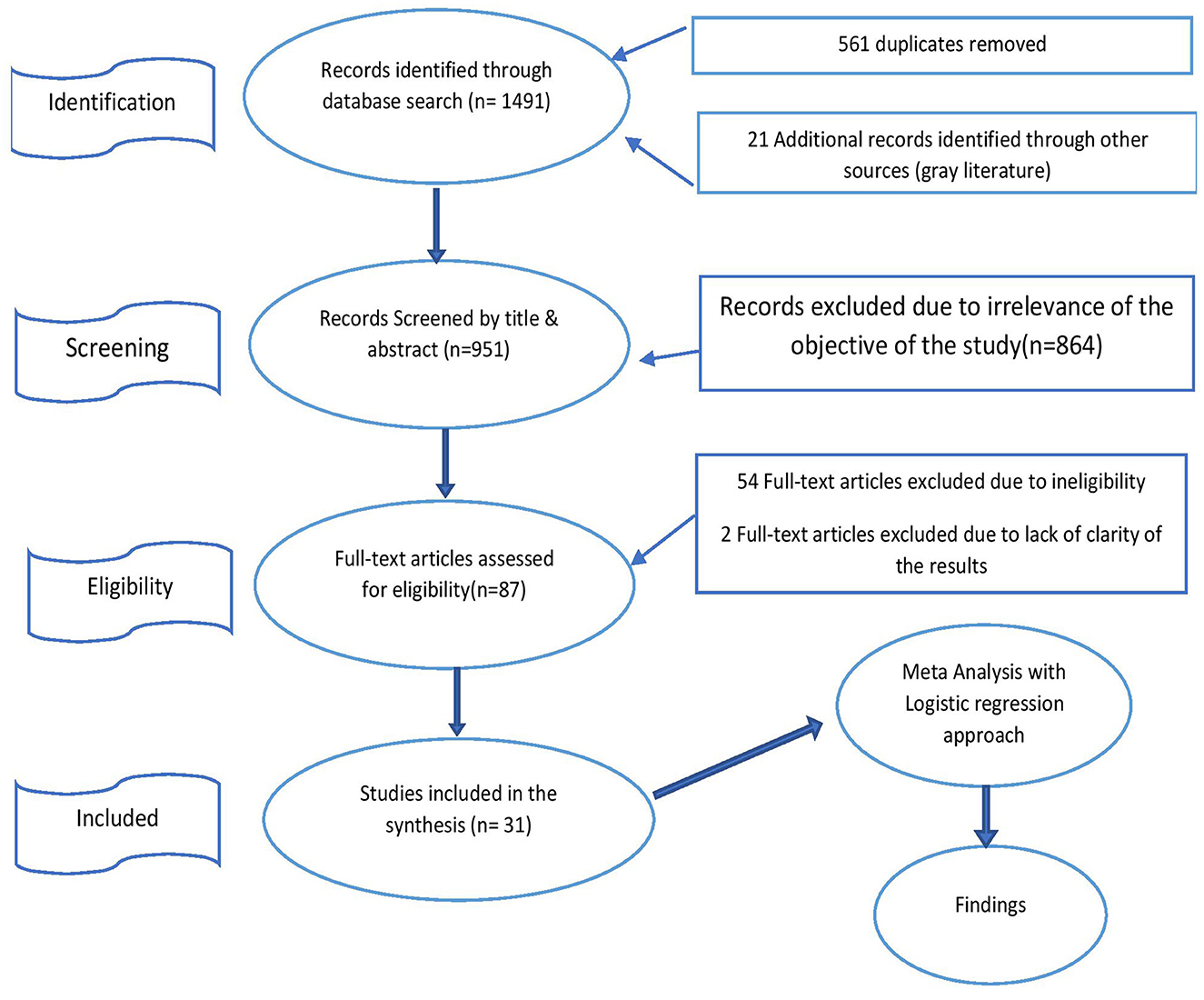
Figure 1. The preferred reporting items for systematic review and meta-analysis flowchart used for meta-analysis and systematic review.
2.1.2 Querying strategy
We used Herzing's publish or perish software to collect the relevant studies. We searched English databases, including Google Scholar, Crossref, Scopus, Web of Science, and African Journals Online. We also browsed through gray literature and conference proceedings related to technical efficiency, with an emphasis on Ethiopia. The search included key terms and keywords independently and/or in combination using the Boolean operators “OR” or “AND.” The searched keywords were (“East Africa Countries” or “Sub-Sahara Africa” or Ethiopia) AND (“Technical Efficiency of Wheat” or “MTE of Wheat” or “Agricultural Performance”) AND (determinants, factors, drives, or causes) in English databases.
2.1.3 Exclusion and inclusion criteria
We comprised studies published in English from 2011 through 2022 that were searched and reviewed from June 1, 2022, to September 30, 2022. We included studies that: (I) include at least one driver or determinant of the TE of wheat (II) uses data from at least one region, or Ethiopia. (III) Are not meta-analyses themselves. (IV) Use household or plot-level data. (V) Reports the coefficients of all control variables. (VI) All studies and those with unclear methods were excluded. (VII) Had a sufficient sample size (n > 50) because of the poor reliability of the estimates. (VIII) Discusses drivers in a conceptual way with empirical analysis. Then, a total of 1,491 articles, book chapters, reports, and 561 studies that were found in the initial search were duplicated and excluded from the list in the first phase. And then, the first searches yielded 951 studies investigating the drivers of TE in wheat output. Finally, considering the abstracts and titles of all the selected papers, the two authors systematically assessed them in two steps. First, inclusion criteria were checked against the titles and abstracts. Then, a recursive search was conducted, and entire texts were reviewed for inclusion. In the final meta-database, there were 31 articles that matched the requirements. Five publications from the database were randomly selected to serve as the pilot for the data abstraction form. The extraction form was modified once the template had been tested.
2.2 Model specifications
The meta-analysis utilizes two models. The fixed-effect approach can only be used if there are key indicators that demonstrate that the included studies are almost identical (Borenstein et al., 2010). But the fixed-effect approach can rarely be used in actual practice. In real-world synthesis, depending on the study, the effect size varies. It is due to a variety of reasons, like differences in participant mixes and intervention implementation. A random-effects approach, therefore, seems to be adequate and effective in the majority of meta-analyses (Gavriilidis et al., 2020). Therefore, pooled estimates of the scale of technical efficiency or the summary effect of a meta-analysis for this paper were estimated by a random effect model.
The study's observed effect, Ti, is determined by the true effect θi plus the within-study error εi. In turn, θi, is determined by the average of all true effects μ and the between-study error ζi. More generally, given any observed effect of Ti,
So, the issue that needed to be addressed was how the weights in the random-effect approach were spread. We must consider two levels of sampling and two sources of errors when using the random effect estimation approach. First, the true effect sizes θ are distributed around μ with a variance of τ2 that corresponds to how the true effects are actually distributed around their mean. Second, for any given θ, the observed effect T will be dispersed about that θ with a variance σ2 that is mostly determined by the study's sample size. Therefore, we must address both within-study (ε) and between-study (ζ) sampling errors when allocating weights to estimate μ.
In a random-effects analysis, the observed variance is divided into two components: within studies and between studies, and both portions are used for determining the weights. The variance is decomposed by first computing the overall (observed) variance and then segregating the within-study variance.
A number of formulas operationalize this logic. If all studies had the same genuine effect, we would calculate Q, which stands for the overall variance, and df, which stands for the expected variance. The excess variance would be the result of the difference, Q – df. Finally, this value would be converted to match the within-study variance in scale. The tau-squared (τ2) value is the most recent one. The Q statistic, which indicates overall variance, is described as follows:
That is, the sum of the “squared deviations” of each research study (Ti) from the overall mean (T). As shown by the “Wi” in the calculation, the “inverse variance” of the study is used to weight each of the squared deviations. A large study that deviates significantly from the mean would have a greater influence on Q than a small study conducted in the same area. An equivalent formula that can be used in calculations is:
Q must now be dissected into its constituent pieces since it represents the overall variance. The predicted value of Q would be the degrees of freedom (df) for the meta-analysis if the only source of variance was a within-study error.
Consequently, we are able to calculate the between-study variation, τ2, as
Where, .
The extra variance (observed minus predicted) makes up the numerator, Q minus df. Due to the fact that Q is a weighted sum of squares, the denominator, C, is a scaling factor. We made sure that the tau-squared was measured using the same unit as the variance within studies by using this scaling factor.
Each study was weighted by the inverse of its variance in this random effect analysis. The distinction is that the variance now consists of both the initial (within-study) variance and the tau-squared variance, which is between-study variance. In particular, the weight given to each study in the random effects model is:
where is the between-studies variance plus the within-study variance for study (i), tau-squared. That is,
Following that, the weighted mean () is calculated as:
This is equal to the sum of the products (effect size times weight) divided by the total weights. The reciprocal of the weights' sum is used to calculate the variance of the combined effect, or
then the square root of the variance is the combined effect's standard error,
For the combined effect, the 95% confidence interval would be calculated as:
Last but not least, if one so desired, the Z-value might be calculated using:
Assuming an effect in the hypothesized direction, the one-tailed p-value is given by
and the two-tailed p-value by
where Φ(Z) is the standard normal cumulative distribution function.
2.3 Empirical estimation models
2.3.1 Publication bias
The fundamental problem with publication bias is that not all completed studies are published, and the selection process is biased. When “editors, reviewers, or researchers” favor statistically significant findings, publication selection occurs (Stanley, 2005).
We employed the funnel plot, the Egger test, or the Begg and Mazumdar rank correlation test to find the publication bias problem. Additionally, we employed the “classic, fail-safe N test” since publication bias raises the possibility that any non-significant papers are omitted from the analysis, which, if true, would cancel out the effect that was observed. The “Trim and Fill” estimating approach would also be used to compute the study's “file drawer” or missing studies problem. The funnel plot is a representation of the relationship between effect size on the horizontal axis and a metric of study size (often standard error or precision) on the vertical axis. The optimum option for the vertical axis is typically the standard error (Sterne and Egger, 2001). Large studies are visible near the top of the “graph” and frequently congregate close to the mean effect size. Smaller studies are shown at the “bottom of the graph” and will be spread throughout a range of values because there is more “sampling variation” in effect-size estimates in smaller studies. Any asymmetry in a funnel plot could be a sign of publication bias.
2.3.1.1 Begg and Mazumdar “rank-correlation” test
The funnel plot illustrates a typical instance of publication bias. Small studies are more “likely” to be included when they demonstrate a relatively large treatment effect, while large studies are more “likely” to be included regardless of their treatment effect. In these conditions, the size of the study and the magnitude of the effect will be inversely correlated. This association was proposed as a test for publication bias by Begg and Mazumdar. Hence, we calculated the rank-order correlation (Kendall's tau b) between the treatment effect and the standard error (which is mostly determined by sample size) for each individual.
2.3.1.2 Egger's test of the intercept
In order to forecast the standardized effect (effect size divided by the standard error), Egger advises utilizing precision, which is the inverse of the standard error, to assess the same bias. In this test, the regression line's slope (B1) captures the magnitude of the treatment effect, whereas the intercept (B0) captures the bias. The rank correlation strategy may not be as advantageous as this one. This could be a stronger test in some situations. Additionally, Egger's linear regression might be used to assess the statistical significance of the funnel plot's asymmetry. Therefore, we employed the inverse variance-weighted Egger's test regression of the observed effect size from trial i (MTEi) on its standard error.
Where Φ is a “multiplicative dispersion parameter” computed from the data which allows for “heterogeneity.”
2.3.1.3 Classic fail-safe N
Instead of merely speculating on the effects of the missing research, Robert Rosenthal suggested that we determine the number of papers necessary to cancel out the effect. There are grounds for alarm if this number is in fact quite tiny. However, if this number is high, we may be confident that the treatment effect is present, even though it may have been overstated due to the omission of some trials. The phrase “Fail-Safe N,” coined by Harris Cooper, refers to the “number of studies” that must be present for the effect to be valid. There are two significant flaws with this approach. In the first place, it makes the assumption that there is no effect on the hidden research, rather than taking into account the likelihood that some of the investigations may have revealed an effect in the opposite direction. The amount of paper needed to reverse the effect may therefore be less than the “fail-safe N.” Second, and maybe more importantly, this approach emphasizes statistical significance. In other words, it may allow us to assert that the treatment effect is not zero, but it raises the question of whether it will remain statistically significant after accounting for the missing trials. Every study's p-value is calculated by the “fail-safe N.” algorithm, which then aggregates these values. The commonly accepted approach nowadays, however, is to calculate an effect size for each study, aggregate the effect sizes, and then calculate the p-value for the total effect. This approach is also the one that this study employs. The two methods typically provide different outcomes.
2.3.1.4 Duval and Tweedie's “Trim and Fill”
A technique created by Duval and Tweedie enables us to impute missing studies. In this study, we identified the likely positions of the missing studies in the funnel plot, included them in the analysis, and then recalculated the cumulative effect. Iteratively trimming the asymmetric results from the right side to identify the unbiased effect gives rise to the term “Trim and Fill,” which refers to the process of filling in the plot with the mean effect by re-inserting the trimmed studies on the right as well as their imputed counterparts on the left. A formal test for asymmetry might also be performed by regressing effect sizes on sample sizes. Similar to the presence of a link between effect sizes and sample sizes, an asymmetric funnel plot can identify publication bias (Card and Krueger, 1995). If there is a substantial negative correlation between sample size and mean technical efficiency estimates in this study, publication bias would be obvious. Therefore, this study used regression to test for asymmetric funnel plots that might indicate publication bias.
where MTEi mean, technical efficiency of study i, SSizei, sample size of study i, and εi error terms.
2.3.2 Analysis of study heterogeneity
A “forest plot” is employed in this investigation to identify heterogeneity. A forest plot offers a detailed visual representation of the findings from each study included in the meta-analysis at a glance.
2.3.3 Determining effect size
According to Hedges and Vevea (1998), Borenstein et al. (2010), Borenstein (2019); Higgins and Thomas (2019), and Borenstein et al. (2021), the articles used in the analysis are thought to constitute a representative sample of all possible studies. Therefore, a conclusion about that universe would be drawn using this approach. In order to determine both parameters for the current study, the software is fed information on the t-statistics and sample size. We were also thinking about the constraints of this approach when used in this manner. In particular, we need enough research to produce a trustworthy estimate of tau-squared in order for the model to function properly. Furthermore, while we can state that the results apply to the field of comparable research, it's not always apparent what exactly falls within that field. We compared the following test statistics across studies to ascertain the effect size of the study.
2.3.3.1 Q-test for heterogeneity
The “null hypothesis,” that all studies included in the analysis have a uniform effect size, is tested by the Q-statistic. If every study had the same true effect size (the number of papers minus 1), the expected value of Q would be equal to the degrees of freedom. Even if the test for heterogeneity is not “statistically significant,” we should infer that the impact size varies between trials if logic dictates that it does.
2.3.3.2 The I-squared statistic
We used I-squared statistics since it is widely believed that I-squared indicates the degree of effect size heterogeneity between studies. In some instances, I-squared has been used in this study to categories the level of variance as low, moderate, or high. I-squared is a percentage, not an exact sum. It demonstrates the relative contribution of sampling error and variation in actual effects to the variation in observed effects. The exact differences in the impacts are unknown to us.
2.3.3.3 Tau-squared and tau
In this investigation, tau-squared is employed to comprehend the variance of true effect sizes.
2.3.4 Meta-regression model; moderator analysis
According to Card and Krueger (1995) and Tesfaye and Tadele (2019), the main goal of a “meta-analysis” of observational studies is not to determine an overall estimate of effect but rather to look into the causes behind variations in estimates between studies and identify patterns of estimates. In a meta-analysis, there are commonly two ways to create the quantitative review. One method is to combine probability values or Z scores; a different method is to combine effect sizes like Cohen's d, correlation coefficients, or effect sizes like Cohen's d. The central premise of this research is that the characteristics of the studies can account for the difference in technical efficiency indices reported in the literature. The following meta-regression model is estimated to look at how technical efficiency scores vary among studies:
where MTEic represents the mean technical efficiency scores from the ith primary study, conducted in the c region in Ethiopia, and ∂0 is the intercept; PUBYEARic is the year in which the research is conducted, which starts from 2011, 2012, 2013, etc. Xmic is a vector of other research attributes used in the meta-regression analysis. It includes, AREA is a categorical variable, equal to one for Tigray, two for Amhara, three for Oromia, four for SNNP, and five for Ethiopia in general; METHOD is a dummy variable that is equal to one if the model is a stochastic frontier and zero otherwise; When a manuscript has been published in a journal, the dummy variable PUBLICATION STATUS is equal to one; otherwise, it is equal to zero. Dummy_2010 is a dummy variable that will be one if the research article covers the years 2010 through 2019 and zero otherwise; a dummy variable called Dummy_2022 has a value of one if the study was carried out between 2020 and 2022 and a value of zero otherwise; the SAMPLE SIZE represents the number of observations used; N0_VARIABLES stands for the number of variables used in the primary study; the final variable, RANGE, represents the difference between the minimum and highest MTE scores reported in the study. The list of moderator variables and their descriptions, which are employed in the study, are displayed in Table 1 below.
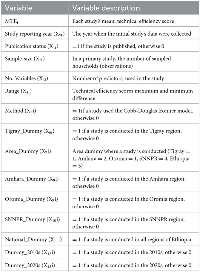
Table 1. Moderator variables and descriptions of them.
3 Discussion and results
3.1 Descriptive statistics and effect size
3.1.1 Descriptive statistics
The descriptive summary of the main studies that were chosen and used in the meta-analysis is shown in Table 2. The average mean efficiency score of the entire set of research (both published and unpublished) is 71.6% and ranges between 48 and 85.8%. Additionally, a detailed examination of Table 3's efficiency estimates by breaking it down according to numerous moderator variables, such as the publication year, the number of variables used, the methodologies used, the range, the region of the study, etc., provided more information. Thus, this measure does not account for the precision (standard deviation and sample size) of each study in estimating the mean efficiency score of households in Ethiopia. Therefore, the average mean efficiency score like this is not the effect size of all the selected studies. Consequently, it is important to use caution when interpreting this outcome. The software for comprehensive meta-analysis assists in recalculating the mean effect size by converting the mean technical efficiency into Fisher's Z estimates to account for relative study size and any deviation from a normal distribution.
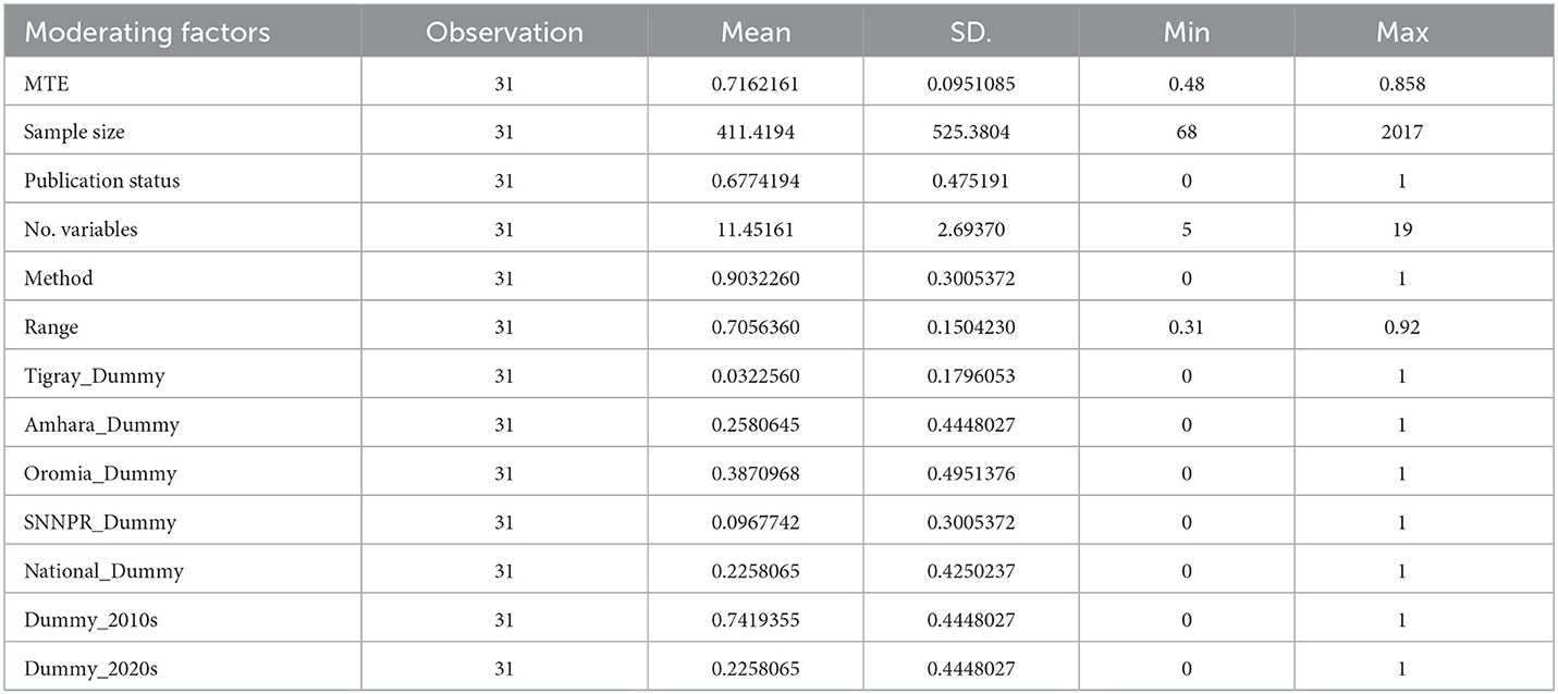
Table 2. The meta-regression model's moderator variables' summary statistics.
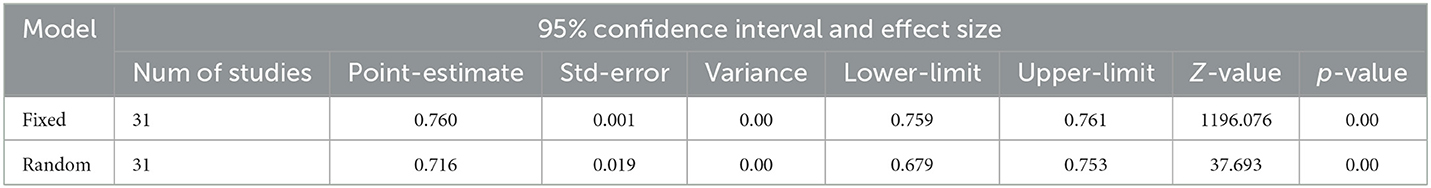
Table 3. Effect size estimated based subgroups as a unit of analysis.
3.1.2 Calculation of effect size of all included studies
Because we are employing the random-effects model, the summary effect size is associated with the mean effect size rather than the common effect size. A 95% confidence interval is used in Table 3 to estimate the mean effect size on the premise that the studies are not homogeneous.
We are calculating the mean of these effects (across all included research) because, in a random-effect model, the true effect size varies from study to study. Thus, the 95% confidence interval for the mean effect size is between 0.679 and 0.753, with a mean of 0.716. The average effect size across all similar trials could lie anywhere within this range. The null hypothesis—that the mean impact size is zero—is tested using the Z-value. The Z-value is 37.693, and the “p-value” is 0.001. We reject the “null hypothesis” using a criterion alpha of 0.050 and come to the conclusion that the mean effect size is not exactly zero in the universe of populations similar to those in the research.
The Prediction Interval (effect size) of future technical efficiency studies; between study variance and other heterogeneity statistics are determined in Table 4. It shows the prediction interval of future technical-efficiency studies along with their “between study variance” and other heterogeneity statistics. The computed test statistics show as follows:
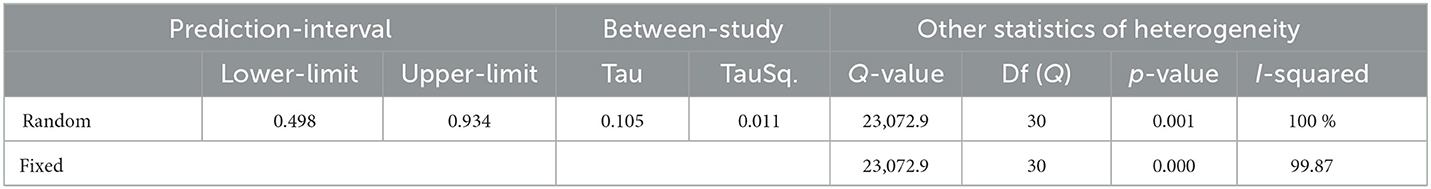
Table 4. Prediction interval of MTE effect-size of future studies.
3.1.2.1 The Q-test for heterogeneity
The anticipated value of Q would be equal to the degrees of freedom (the number of studies minus 1) if the genuine effect sizes of all studies were equal. The result in Table 4 shows that the Q-value is 23,072.88 with 30 df and a p-value < 0.001. We can reject the null hypothesis that the true effect size is the same across all of these trials using a criteria alpha of 0.100. Hence, the fact that the effect magnitude varies among studies is supported by empirical data in this circumstance. Researchers occasionally believe that the Q-statistic or the associated p-value provide information on the degree of variation in the effects. This is incorrect. Only the “Is there any variation in effects?” question is addressed by the Q-value and p-value. In most cases, the key concern is, “How much does the effect size vary?” The prediction interval addresses this query, which could be covered later.
3.1.2.2 The “I-squared” statistic
Many individuals believe that I-squared represents how much the “effect size” varies among studies. The 100% I-squared statistic indicates that some 100% of the variance in observed effects actually represents variance in true effects as opposed to sampling error. The prediction interval, which is described below, is the statistic that indicates how widely the effect size fluctuates.
3.1.2.3 Tau-squared and tau
The variation of actual effect sizes, tau-squared, is 0.011 in raw units. Tau, the true effect size standard deviation, is 0.105 in raw units. Therefore, the study further revealed that both published and unpublished researches effect size variation is very low and close to the actual effect size.
3.1.2.4 Prediction interval (future studies)
The assumption that the effects are normally distributed around the mean is one of several that affect the prediction interval's accuracy. Therefore, it would be crucial to determine whether there are truly observable effects that support this conclusion if the prediction interval includes effects that suggest an intervention is hazardous (DerSimonian and Laird, 1986; Higgins and Thompson, 2002; Higgins et al., 2003; Higgins, 2008; IntHout et al., 2016; Borenstein et al., 2017; Higgins and Thomas, 2019; Borenstein, 2020). We could determine that the prediction interval is between 0.498 and 0.934 if we assume that the true-effects are normally distributed (in raw units). And the true effect size in 95% of all comparable populations falls within this interval. The interval could be misleading, though, if our estimates of the mean, standard deviation, and/or effects don't follow a “normal distribution.”
3.2 Meta-regression analysis
We have to investigate the publication bias and heterogeneity issues using a funnel plot, regression model, and forest plot before applying the meta-regression model.
3.2.1 Exploring publication bias
The publication bias is shown either visually using the funnel plot, the Egger test, or the Begg and mazumdar rank correlation test. In addition, the “Trim and Fill” and classic fail-safe N test estimation tests are given below.
3.2.1.1 Funnel plot test result
Figures 2, 3 show the funnel plot for the mean technical efficiencies of the sampled research, stratified by publication type for both standard error and precision. Without publication bias, we would anticipate a symmetrical distribution of the studies around the aggregate effect size. The bottom of the plot, however, should show a higher concentration of studies on one side of the mean (the vertical grid line) than the other if bias exists. This would be in line with the reality that smaller studies (placed at the bottom) are more “likely” to be published if they have “larger than” the “average effects,” increasing their likelihood of satisfying the need for statistical significance. Figures 2, 3 shown below are found to be distributed symmetrically about the total effect size. Further, the majority of the studies, both published and unpublished, on the right and left sides are evenly distributed. This revealed that the study has not found any publication bias. Further, various diagnostic tests are also performed to quantify or augment this display.
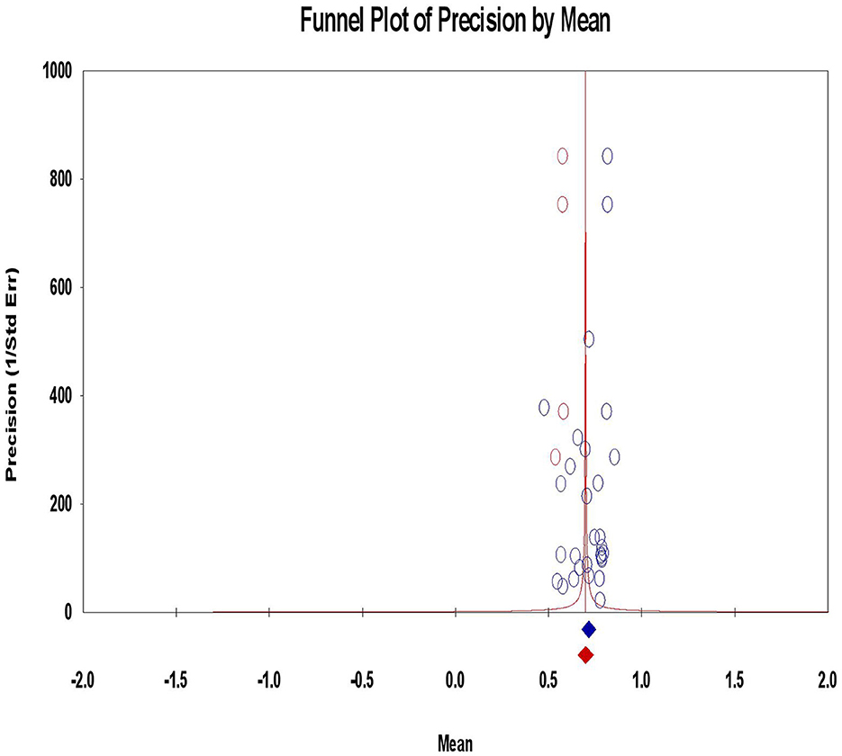
Figure 2. The funnel plot (precision of studies vs. mean), stratified by publication type for the mean technical efficacy of the sampled research. The majority of the research, both published and unpublished, are evenly distributed across the right and left sides of the grid line.

Figure 3. The funnel plot (standard error vs. mean) stratified by publication type for the mean technical efficacy of the sampled research. The researches are evenly distributed across the right and left sides of the grid line.
3.2.1.1.1 Classic “fail-safe N” test
The outcome of the classic “fail-safe N” test is displayed in Table 5. Data from 31 papers were used in this analysis, which resulted in a z-value of 843.87609 and a 2-tailed p-value of 0.00000. The fail-safe-N value is 5,746,727.0. This implies that for the total two-tailed p-value to exceed 0.050, we should need to find and add 5,746,727 “null” studies. To put it another way, the effect would have to be eliminated if there were 185,378.3 missing studies for every study that was seen. A 31-study meta-analysis demonstrating that one should not be concerned that the entire observed effect size is an artifact of a bias to modify the mean effect size, which is implausible.

Table 5. Classic “fail safe N” test result.
3.2.1.1.2 Begg and Mazumdar's “rank correlation” test
The results of the Begg and Mazumdar “rank correlation” test are displayed in Table 6. Although a substantial association raises the possibility of bias, it does not specifically address its effects. A non-significant association, on the other hand, may not be indicative of bias because of poor statistical power. In this instance, the one-tailed p-value (recommended) is 0.36057, while the two-tailed p-value (based on continuity-corrected normal approximation) is 0.72115. Kendall's tau b (adjusted for ties, if any) is −0.04526. Generally speaking, the test result can also show that the study was free of publication bias.
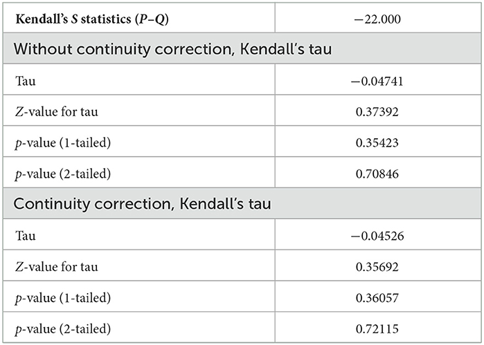
Table 6. Begg and Mazumdar “rank-correlation” test.
3.2.1.1.3 Egger's test of the intercept
Regression of the Egger test according to Table 7's results: the intercept (B0) is −12.19777 with a 95% confidence interval of (−26.68053, 2.28499), t = 1.7255, and df = 29. The recommended one-tailed p-value is 0.04781, while the two-tailed p-value is 0.09562. Egger's test of the intercept favors the informal test result and fails to reject the hypothesis of zero intercepts indicating no publication bias. In light of the fact that the problem is not present in this research, the result further shows that the mean and effect size would not be adjusted for publication bias.
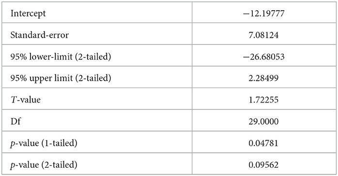
Table 7. Results of the Egger's regression test.
3.2.1.1.4 Duval and Tweedie's “Trim and Fill”
Based on a random effects model, the program searches solely for studies that are absent on the left side of the mean effect. The result suggests that four research exists according to these variables estimate. The fixed effect model pooled studies are shown in Table 8, with a 95% confidence interval and point estimate of 0.76131 and (0.75881, 0.76131) respectively. The imputed point estimate using Trim and Fill is 0.69131 (0.69033, 0.69229). The pooled studies' point estimate and 95% confidence interval for the random-effects model are 0.71615 (0.67891, 0.75338). The imputed point estimate using Trim and Fill is 0.69933 (0.65792, 0.74075). Additionally, as our model is a random effect model, the test confirms that the mean effect size is equal to the MTE effect size of the outcome. As a result, we can draw the conclusion that the papers chosen for the meta-regression analysis can be trusted to accurately represent the distribution of technical efficiency in Ethiopian agriculture for further study.
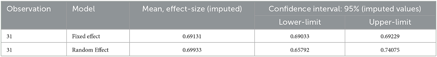
Table 8. Trim and Fill test result.
3.2.2 Detecting heterogeneity among studies
The random effect meta-analysis estimate in Figure 4 shows the forest plot for the mean technical efficiency for each study by kind of publication, i.e., journal (=1) or thesis (=0). The area of each square in the plots corresponds to the study's weight in the meta-analysis and represents the mean technical efficiency evaluated in each of the 31 observations. According to Figure 4, research that has been published in journals has an average mean technical efficiency that is lower than studies that have not been published.
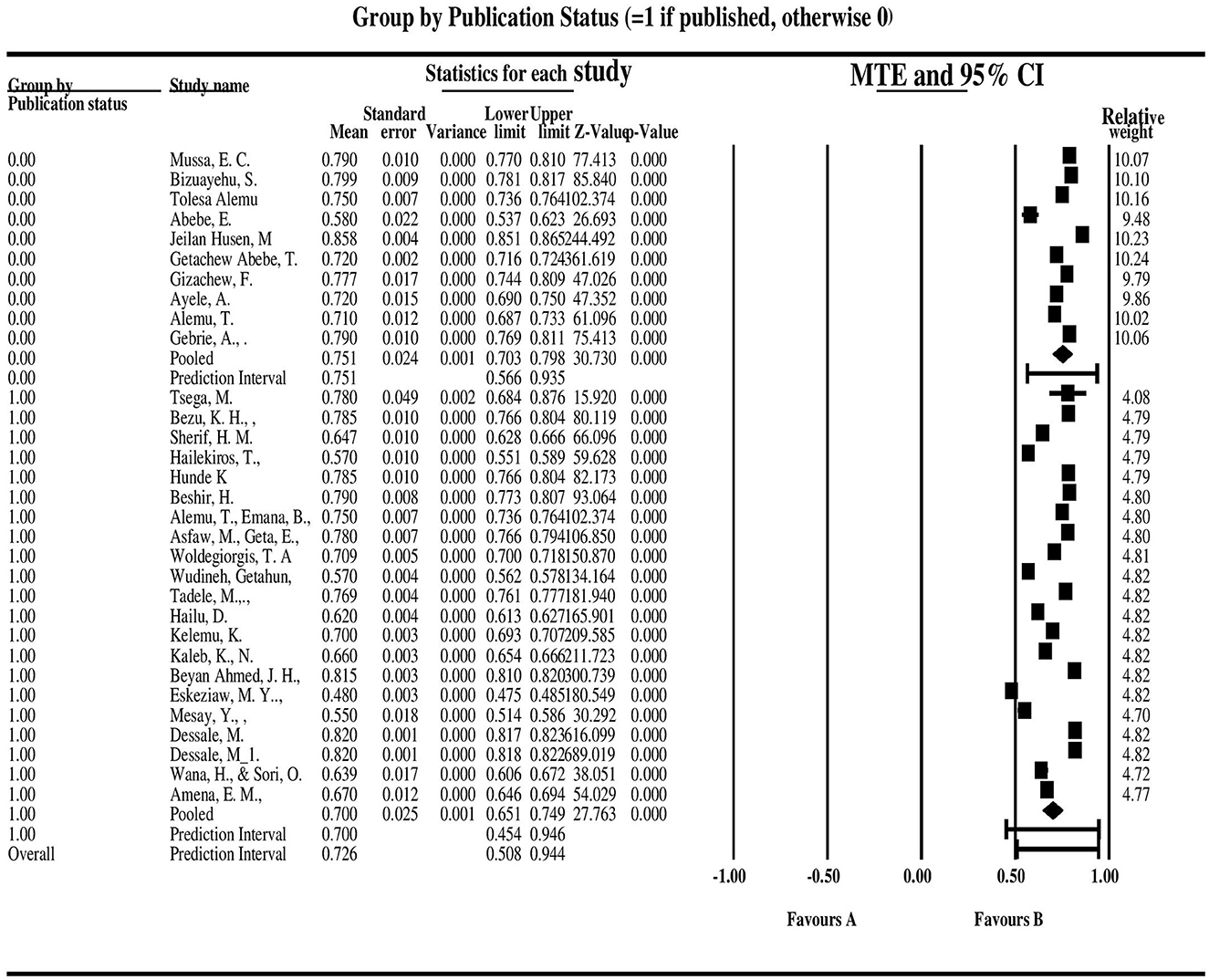
Figure 4. The forest plot for the mean technical efficiency for each study by kind of publication, i.e., journal (=1) or thesis (=0).
Additionally, the “forest plot” shows that studies that have not yet been published in journals are less heterogeneous (based on the square distribution), while research that has been published in journals is more heterogeneous. Due to the heterogeneity of the published studies, the overall meta-analysis average mean technical efficiency estimate is significantly diverse (pooled MTE = 72.6%). Furthermore, Figure 5 shows that, with a 95% confidence interval between 0.68 and 0.75, the mean technical efficiency effect size is 0.72. This further demonstrates that in 95% of all comparable groups, true effect size lies within the interval of 0.50 to 0.93.
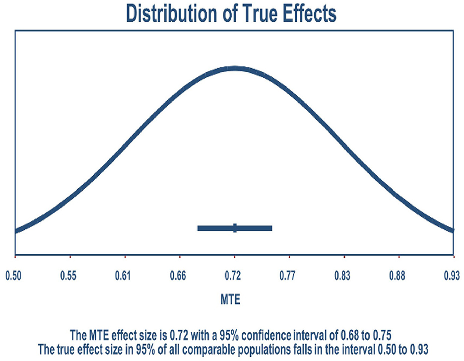
Figure 5. The true effect size distribution of all the sampled studies and their effect size.
3.3 Meta-regression analysis: moderator analysis
Meta-regression in this section answers possible factors for variations in effect sizes among studies. The sample papers were assessed over a 12-year period (2011–2022). The MRA in Table 9 is based on the random effect model. The regression result in Table 9 displays that the 31 mean technical efficiency studies included in the analysis have shown different efficiency scores because they differ in sample size, methods employed, publication status, range, and location of the study. The following is a summary of the main conclusions concerning the variables influencing the variations in efficiency ratings of families producing wheat in Ethiopia from earlier studies.
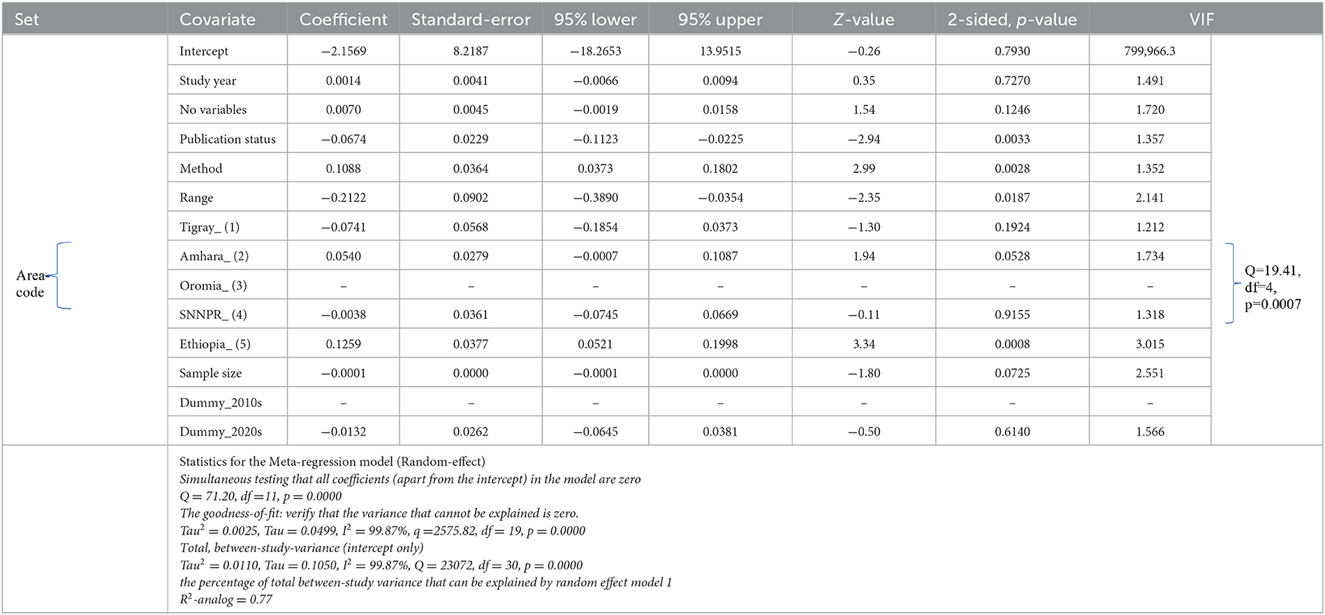
Table 9. Meta-regression analysis result.
According to the estimates, the result of meta-regression shows that study characteristics such as methods employed, publication status, range of the efficiency scores, location of the study, and sample size significantly affect the variation in effect size among the sample studies at a 10 % significant level. Implying that, other things remaining constant, a 1 % change in these regressors leads to a 10.88%, 6.74%, 21.22%, 0.01% change in the MTE scores across studies in Ethiopia respectively. In addition, the MTE score in studies is also affected by the location in which the study is conducted.
3.3.1 The method employed
According to the meta-regression estimates, the parameter estimates of models using stochastic frontiers are positive and significant and have different technical efficiency scores than deterministic models. This outcome is in line with a priori predictions that deterministic models have higher inefficiency scores than stochastic frontiers.
In addition, empirical research by Ekanayake and Jayasuriya (1987) revealed that the bias in deterministic techniques is unknown and tends to exaggerate the level of technical inefficiency on the whole. Accordingly, these tests demonstrate that the chosen frontier studies that were used in the Meta-regression analysis can be trusted to accurately represent the distribution of technical efficiency in Ethiopian agriculture for further study.
3.3.2 Publication status of a study
The mean TE scores across trials are negatively and significantly impacted by journal-publication status, implying that the mean technical efficiency of studies published in a journal was found with lower MTE scores than those unpublished in a journal (Thesis) in Ethiopia. This result is in line with the findings of Tesfaye and Tadele (2019) and in contrast with the finding of Ogundari (2014).
3.3.3 Area of the research
Location effect or “area of the study,” the overall effect of all regions (Tigray, Amhara, Oromia, SNNPR, Ethiopia) with a combined p-value of 0.0007 (Q = 19.41, df = 4) is significant and different across regions. The study is also in line with Tesfaye and Tadele (2019). The empirical results also show that the mean efficiency score in the Tigray region is the lowest, followed by SNNPR, Amhara, and Oromia. This shows that systematic variation in the reported “mean efficiency” estimates based on particular attributes in the study is largely caused by geographical differences, which may be significant in some cases.
3.3.4 Range
The “econometric result” shown in Table 9 also reveals that the range of the mean “technical efficiency” scores significantly affects MTE estimates across studies. This study is in line with Ogundari and So (2009), Tekalign (2021).
3.3.5 Sample size
The meta-regression results also confirm that the number of observations being examined in each study affects the mean efficiency estimate across studies: the average mean technical efficiency score decreases as more observations are included. The likelihood that the new households were inefficient is greater than the probability that they were efficient as the number of observations rises. As a result, the “mean efficiency” which is computed by dividing the total number of households by the average efficiency scores of all wheat growers will probably decline. This research supports Tesfaye and Tadele's (2019) findings.
However, the number of variables used in the studies, and the year of the study conducted have insignificant impacts on the mean technical efficiency of studies in Ethiopia. In the years to come, when more cutting-edge studies become available, we propose that additional studies on Ethiopia's agriculture sector are important and may add to that discussion.
4 Conclusion
This review epitomizes the first endeavor to use a meta-analysis and a systematic review to scrutinize the mean technical efficiency of wheat farming in Ethiopian agriculture. Between 2011 and 2022, 31 studies utilizing farm- and household-level data from Ethiopia were assessed. Using random-effect estimation methods, the mean effect size is 71.6% and the farm-level MTE scores from all the research analyzed to have a 95% confidence interval of 67.9%−75.3%. It implies that there is still hope for boosting Ethiopia's wheat farming productivity. The results further indicate that, with the same level of input use, Ethiopian agricultural farming productivity still has room to rise by 28.4%. Therefore, increasing the technical efficiency of households should be a key priority on nations' national agendas in order to comprehend the nutritional demands of high-risk groups in Ethiopia. The findings also reveal that, at the 10% level of significance, study attributes such as the methods used, publication status, range of efficiency scores, study location, and sample size have a substantial impact on the variation in effect size among the sample studies in Ethiopia. The results also urge academics and researchers to be observant in order to pinpoint study-specific characteristics that are crucial for duplicating farm-level efficacy. Therefore, as it is systematically reviewed in this study, the researchers should take into account additional factors that have an impact on the productivity of the agricultural sector and agricultural efficiency, such as labor, fertilizer cost, cooperative membership, access to credit, size of cultivated land, access to machinery, extension service access, educational level, agricultural farm size, and family size. From a policy point of view, more precise TE estimates of wheat yield are essential for directing policy choices and supporting the newly announced economic development plan (2021–2030), a 10-year strategy, where agriculture is the top priority. With an ambitious strategy to produce enough wheat for everyone, end imports, and make a commitment to start selling wheat to nearby countries, among other things.
Data availability statement
The raw data supporting the conclusions of this article will be made available by the authors, without undue reservation.
Author contributions
AT conceived of the study's concept, planned it out, gathered the data, used software to analyses it, reviewed the results, and wrote the initial manuscript. HM conceived of the study's concept, oversaw the research, gave direction throughout the process, and contributed critical revisions and writing assistance. All authors agreed to bear responsibility for the whole article after reading and approving the final manuscript.
Conflict of interest
The authors declare that the research was conducted in the absence of any commercial or financial relationships that could be construed as a potential conflict of interest.
Publisher's note
All claims expressed in this article are solely those of the authors and do not necessarily represent those of their affiliated organizations, or those of the publisher, the editors and the reviewers. Any product that may be evaluated in this article, or claim that may be made by its manufacturer, is not guaranteed or endorsed by the publisher.
Footnotes
1. ^Mean Technical Efficiency (MTE): The ability of the household to harvest far more return than is achievable from its resources is known as technical efficiency. If a household produces greater production compared to another at the same input utilization and technology level, it is considered to be more technically efficient. MTE, thus, refers to a household's overall average of its entire technical efficiency.
References
Abebe, E. (2015). Comparison of profitability and production efficiency of major cereal crops in Adama Woreda, Central Ethiopia [Doctoral dissertation]. Harar: Haramaya University.
Alemu, T. (2020). Wheat Production Efficiency and Profitability Ethiopian Institute of Agricultural research. Available online at: http://hdl.handle.net/123456789/3342
Alemu, T., Emana, B., Haji, J., and Legesse, B. (2014). Smallholder wheat production efficiency in selected agroecological zones of Ethiopia: a parametric approach. J. Econ. Sustain. Dev. 5, 155–163.
Amena, E. M., and Mulatu, G. (2020). Technical efficiency of wheat producing farmers in the case of bale zone of Oromia region, Ethiopia: an application of stochastic frontier approach. J. Econ. Sustain. Dev. 11. doi: 10.7176/JESD/11-11-07
Asfaw, M., Geta, E., and Mitiku, F. (2019). Economic efficiency of smallholder farmers in wheat production: the case of Abuna Gindeberet district, Oromia National Regional State, Ethiopia. Int. J. Environ. Sci. Nat. Resour. 16, 41–51. doi: 10.22004/ag.econ.285931
Ayele, A., Haj, J., and Tegegne, B. (2019). Technical efficiency of wheat production by smallholder farmers in Soro district of Hadiya zone, southern Ethiopia. East Afr. J. Sci. 13, 113–112.
Beshir, H. (2016). Technical efficiency measurement and their differential in wheat production: the case of smallholder farmers in South Wollo. IJEBF 4, 1–16.
Beyan Ahmed, J. H., and Geta, E. (2013). Analysis of farm households' technical efficiency in production of smallholder farmers: the case of Girawa District, Ethiopia. J. Agric. Environ. Sci. 13, 1615–1621. doi: 10.5829/idosi.aejaes.2013.13.12.12310
Bezu, K. H., Chala, B. W., and Itticha, M. W. (2021). Economic efficiency of wheat producers: the case of Debra Libanos District, Oromia, Ethiopia. Turk. J. Agric.-Food Sci. Technol. 9, 953–960. doi: 10.24925/turjaf.v9i6.953-960.4244
Bizuayehu, S. (2012). Economic Efficiency of Wheat Seed Production: Amhara Region, Ethiopia. Harar: Haramaya University.
Borenstein, M. (2019). Common Mistakes in Meta-Analysis and How to Avoid Them. Frederick, MD: Biostat, Inc.
Borenstein, M. (2020). Research note: in a meta-analysis, the I2 index does not tell us how much the effect size varies across studies. J. Physiother. 66, 135–139. doi: 10.1016/j.jphys.2020.02.011
Borenstein, M., Hedges, L. V., Higgins, J. P., and Rothstein, H. R. (2010). A basic introduction to fixed-effect and random-effects models for meta-analysis. Res. Synth. Methods 1, 97–111. doi: 10.1002/jrsm.12
Borenstein, M., Hedges, L. V., Higgins, J. P. T., and Rothstein, H. R. (2021). Introduction to Meta-Analysis, 2nd ed. Hoboken, NJ: Wiley. doi: 10.1002/9781119558378
Borenstein, M., Higgins, J. P., Hedges, L. V., and Rothstein, H. R. (2017). Basics of meta-analysis: I2 is not an absolute measure of heterogeneity. Res. Synth. Methods 8, 5–18. doi: 10.1002/jrsm.1230
Card, D., and Krueger, A. B. (1995). Time-series minimum-wage studies: a meta-analysis. Am. Econ. Rev. 85, 238–243.
DerSimonian, R., and Laird, N. (1986). Meta-analysis in clinical trials. Control. Clin. Trials 7, 177–188. doi: 10.1016/0197-2456(86)90046-2
Dessale, M. (2018). Measurement of technical efficiency and its determinants in wheat production: the case of smallholder farmers in wogidi district, south wollo zone Ethiopia. Food Sci. Qual. Manag 81.
Dessale, M. (2019). Analysis of technical efficiency of small holder wheat-growing farmers of Jamma district, Ethiopia. Agric. Food Secur. 8, 1. doi: 10.1186/s40066-018-0250-9
Ekanayake, S. A. B., and Jayasuriya, S. K. (1987). Measurement of firm-specific technical efficiency: a comparison of methods. J. Agric. Econ. 38, 115–122. doi: 10.1111/j.1477-9552.1987.tb01032.x
Eskeziaw, M. Y., Ketema, M., Haji, J., and Bekele, K. (2021). Production efficiency of major crops among smallholder farmers in Central Ethiopia. J. Agribus. Rural Dev. 61, 235–245. doi: 10.17306/J.JARD.2021.01391
Gavriilidis, P., Wheeler, J., Spinelli, A., de 'Angelis, N., Simopoulos, C., and Di Saverio, S. (2020). Robotic vs laparoscopic total mesorectal excision for rectal cancers: has a paradigm change occurred? A systematic review by updated meta-analysis. Colorectal Dis. 22, 15061517. doi: 10.1111/codi.15084
Gebrie, A., and Mada, M. (2018). Technical Efficiency of Smallholder Wheat Producers in Simada District of Amhara Region, Ethiopia. doi: 10.7176/DCS/10-1-01
Getachew Abebe, T. (2021). Technical efficiency, market participation, and Food security of wheat producers in Northern Shewa Zone of Amhara region, Central Ethiopia [Doctoral dissertation]. Harar: Haramaya University. doi: 10.5539/sar.v9n3p77
Gizachew, F. (2017). Economic Efficiency of Smallholder Wheat Producers in Damot Gale District, Southern Ethiopia [Doctoral dissertation]. Harar: Haramaya University.
Hailekiros, T., Gebremedhin, B., and Tadesse, T. (2018). Technical inefficiency of smallholder wheat production system: empirical study from Northern Ethiopia. Ethiop. J. Econ. 27, 151–171.
Hailu, D. (2020). Determinants of Technical efficiency in wheat production in Ethiopia. Int. J. Agric. Econ. 5, 218. doi: 10.11648/j.ijae.20200505.19
Havránek, T., Stanley, T. D., Doucouliagos, H., Bom, P., Geyer-Klingeberg, J., Iwasaki, I., et al. (2020). Reporting guidelines for meta-analysis in economics. J. Econ. Surv. 34, 469–475. doi: 10.1111/joes.12363
Hedges, L. V., and Vevea, J. L. (1998). Fixed and random-effects models in meta-analysis. Psychol. Methods 3, 486–504. doi: 10.1037/1082-989X.3.4.486
Higgins, J. P. (2008). Commentary: heterogeneity in meta-analysis should be expected and appropriately quantified. Int. J. Epidemiol. 37, 1158–1160. doi: 10.1093/ije/dyn204
Higgins, J. P., and Thompson, S. G. (2002). Quantifying heterogeneity in a meta-analysis. Stat. Med. 21, 1539–1558. doi: 10.1002/sim.1186
Higgins, J. P., Thompson, S. G., Deeks, J. J., and Altman, D. G. (2003). Measuring inconsistency in meta-analyses. BMJ 327, 557–560. doi: 10.1136/bmj.327.7414.557
Higgins, J. P. T., Thomas, J., Chandler, J., Cumpston, M., Li, T., Page, M. J., . (eds.). (2019). Cochrane Handbook for Systematic Reviews of Interventions, 2nd Edn. Hibiken, NJ: Wiley. doi: 10.1002/9781119536604
Hunde, K. (2019). Technical efficiency of smallholder farmers wheat production: the case of Debra Libanos District, Oromia National Regional State, Ethiopia. Open Access J. Agric. Res. 4. doi: 10.23880/oajar-16000232
International Trade Administration (2022). Ethiopian-Agriculture Sector. Washington, DC: Department of Commerce, USA.
IntHout, J., Ioannidis, J. P. A., Rovers, M. M., and Goeman, J. J. (2016). Plea for routinely presenting prediction intervals in meta-analysis. BMJ Open 6, e010247. doi: 10.1136/bmjopen-2015-010247
Jeilan Husen, M., and Fentaw, S. (2019). Analysis of Economic Efficiency of Wheat Production: The Case of Robe District, Arsi Zone, Oromia National Regional State, Ethiopia (Doctoral dissertation). Harar: Haramaya University.
Kaleb, K., and Workneh, N. (2016). Analysis of levels and determinants of technical efficiency of wheat producing farmers in Ethiopia. Afr. J. Agric. Res. 11, 3391–3403. doi: 10.5897/AJAR2016.11310
Kelemu, K. (2016). Impact of mobile telephone on technical efficiency of wheat growing farmers in Ethiopia. Int. J. Res. Stud. Agric. Sci. 2, 1–9. doi: 10.20431/2454-6224.0207001
Mesay, Y., Tesafye, S., Bedada, B., Fekadu, F., Tolesa, A., and Dawit, A. (2013). Source of technical inefficiency of smallholder wheat farmers in selected waterlogged areas of Ethiopia: a translog production function approach. Afr. J. Agric. Res. 8, 3930–3940. doi: 10.5897/AJAR12.2189
Ministry of Agriculture (2021). Agricultural Sector Performance, Addis Ababa. Addis Ababa: Ministry of Agriculture.
Mussa, E. C. (2011). Economic Efficiency of Smallholder Major Crops Production in the Central Highlands of Ethiopia [Doctoral dissertation]. Nairobi: Egerton University.
Ogundari, K. (2014). The paradigm of agricultural efficiency and its implication on food security in Africa: what does meta-analysis reveal? World Dev. 64, 690–702. doi: 10.1016/j.worlddev.2014.07.005
Ogundari, K., and So, O. J. O. (2009). An examination of income generation potential of aquaculture farms in alleviating household poverty: estimation and policy implications from Nigeria. Turk. J. Fish. Aquat. Sci. 9, 39–45.
Sherif, H. M. (2020). Economic efficiency of crop production in Gurage zone: the case of Abeshige Woreda, Snnpr Ethiopia. Int. J. Adv. Eng. Res. Sci. 7. doi: 10.22161/ijaers.710.7
Stanley, T. D. (2005). Beyond publication bias. J. Econ. Surveys 19, 309–345. doi: 10.1111/j.0950-0804.2005.00250.x
Sterne, J. A., and Egger, M. (2001). Funnel plots for detecting bias in meta-analysis: guidelines on choice of axis. J. Clin. Epidemiol. 54, 1046–1055. doi: 10.1016/S0895-4356(01)00377-8
Tadele, M., Wudineh, G., Ali, C., Agajie, T., Tolessa, D., Solomon, A., et al. (2018). Technical efficiency and yield gap of smallholder wheat producers in Ethiopia: a stochastic Frontier analysis. Afr. J. Agric. Res. 13, 1407–1418. doi: 10.5897/AJAR2016.12050
Tekalign, F. M. (2021). Technical efficiency of Ethiopian agriculture: a meta-analysis. J. Agric. Res. Pest. Biofertil. 1.
Tesfaye, S., and Tadele, M. (2019). A synthesis of Ethiopian agricultural technical efficiency: a meta-analysis. Afr. J. Agric. Res. 14, 559–570. doi: 10.5897/AJAR2017.12729
Tsega, M. (2019). Analysis of levels and determinants of technical efficiency of wheat producing farmers: the case of east Gojame zone, Amhara Region, Ethiopia. Int. J. Dev. Res. 9, 31400–31404.
Wana, H., and Sori, O. (2020). Factors affecting the productivity of wheat production in Horo district of Oromia region, Ethiopia. J. Poverty Invest. Dev. 52, 1–13. doi: 10.7176/JPID/52-01
Wang, C., Wen, W., Zhang, H., Ni, J., Jiang, J., Cheng, Y., et al. (2023). Anxiety, depression, and stress prevalence among college students during the COVID-19 pandemic: a systematic review and meta-analysis. J. Am. Coll. Health 71, 2123–2130. doi: 10.1080/07448481.2021.1960849
Woldegiorgis, T. A. (2019). Stochastic Production Frontier Analysis of Small Holder Farmers' Technical Efficiency: Evidence from Womberma District Wheat Producers', Amhara Regional State, Ethiopia. IJRAR- International Journal of Research and Analytical Reviews.
Keywords: meta-regression, systematic review, random-effect, mean technical efficiency, wheat, Ethiopia
Citation: Mulusew A and Hong M (2023) A systematic review and meta-regression analysis of technical efficiency in Ethiopian wheat farming. Front. Sustain. Food Syst. 7:1214278. doi: 10.3389/fsufs.2023.1214278
Received: 12 May 2023; Accepted: 23 October 2023;
Published: 16 November 2023.
Edited by:
Everlon Cid Rigobelo, São Paulo State University, BrazilReviewed by:
Zlati Monica Laura, Dunarea de Jos University, RomaniaRomeo-Victor Ionescu, Dunarea de Jos University, Romania
Copyright © 2023 Mulusew and Hong. This is an open-access article distributed under the terms of the Creative Commons Attribution License (CC BY). The use, distribution or reproduction in other forums is permitted, provided the original author(s) and the copyright owner(s) are credited and that the original publication in this journal is cited, in accordance with accepted academic practice. No use, distribution or reproduction is permitted which does not comply with these terms.
*Correspondence: Mingyong Hong, aG9uZ21pbmd5b25nQDE2My5jb20=