Exploring the dynamics of arrivals and prices volatility in onion (Allium cepa) using advanced time series techniques

Modeling the arrivals and prices of agricultural commodities is an essential requirement for farmers, consumers, and governmental organizations to make informed decisions. This is particularly important for perishable commodities such as vegetables, where spoilage can lead to significant losses for farmers and have a ripple effect on supply and demand dynamics. Volatility in the arrivals and prices of vegetables like onion is a serious issue affecting the common person in different ways. The study attempts to employ different time series models like the autoregressive integrated moving average (ARIMA), Artificial neural network (ANN), hybrid, and ensemble empirical mode decomposition (EEMD) techniques to analyze the pattern and trend of onions in Chandigarh and Delhi markets. From the results of the study, the amount of volatility in the data was found to range from medium to high among the markets. Decomposition techniques such as EEMD-ARIMA and EEMD-ANN performed better for the study data with the least mean absolute percentage error (MAPE) values, such as 17.74 and 6.78% for arrivals and 9.76 and 10.24% for prices at Chandigarh and Delhi markets, respectively. The EEMD techniques exceled in handling the non-linearity and non-stationarity by decomposing the data into different intrinsic modes and a residual, providing a better understanding of the fluctuation levels of data.

Introduction

The arrivals and prices of agricultural commodities are integral to farming communities and hold substantial interest for stakeholders. They exert a direct influence on the selling and purchasing power of the populace, particularly small and marginal farmers, by impacting their real income (Allen, 1994). The uncertainty of production, poor infrastructure, perishable nature, seasonality of production, and hikes in fuel and transport costs are the major reasons behind the fluctuations in the arrivals and prices of agricultural commodities (Paul et al., 2015). In recent times, India has witnessed some serious fluctuations in the arrivals and prices of vegetables, particularly onions. The prices of onions are highly volatile due to their high demand and unstable supply, which indirectly affects their production across many places (Rakshit et al., 2021). Onions (Allium cepa) occupy a preeminent position as a fundamental ingredient in diverse cuisines and are among the most widely grown and globally consumed vegetables. India is the second-largest onion producer in the world after China, accounting for around 20% of the global onion production. The major onion-cultivating (Kumar et al., 2022) states in India are Maharashtra, Karnataka, Gujarat, Madhya Pradesh, and Bihar. Although the crop can be grown in different seasons, the onion supply chain is susceptible to a range of external factors, such as weather disturbances and policy regulations (Saxena et al., 2019). Furthermore, the perishable nature of onions and the limited availability of modern cold storage facilities pose additional challenges for the supply chain. As a result of these factors, the price of onions is prone to exhibiting high volatility. Thus, the volatility in onions can impose substantial issues for both farmers and consumers (Kumar et al., 2021), making it harder to stabilize prices and maintain an adequate supply to meet the rising demand for fresh produce. Therefore, timely forecasting of the arrivals and prices is essential to understand the pattern of fluctuations to give assured foresight on production and marketing in the future (Areef et al., 2020). All of these can support the farmers and other stakeholders to manage the risks and optimize their operations by ensuring a stable supply of fresh produce for consumers.

Forecasting the arrivals and prices of agricultural commodities is crucial and difficult as they are prompted by various factors such as an imbalanced demand and supply (Arjun, 2013), problems of hedging and speculation, and various services imposed on goods. In addition, many random factors like drought, flood, famine, the incidence of pests, and diseases also have an effect. The recent outbreak of COVID-19 has worsened the pattern of demand and supply. All these factors have resulted in high fluctuations in the arrivals and prices, imposing the characteristics (Paul et al., 2023) of non-linearity, non-stationarity, and noise on the data. In recent times, different time series models have been introduced which can handle the problems of volatility better than conventional models. Autoregressive integrated moving average (ARIMA) is a commonly used traditional time series method that can handle the linearity in the data (Pardhi et al., 2018). Artificial neural networks (ANN) are regarded as black box techniques of machine learning models (Singh, 2008) because of their complex internal structure, numerous interconnected nodes, lack of transparency in the training process, and ability to capture complex non-linear relationships, (Anjoy et al., 2017) which makes it challenging to understand the prediction process and interpret the results. Additionally, the absence of explicit rules further reinforces the notion of ANNs being black boxes. Generalized autoregressive conditional heteroskedasticity (GARCH) is a variance function model that can be used only when the error variance of the model is autocorrelated (Kumar and Thenmozhi, 2014). It can be used as a hybrid technique with ARIMA as the mean model. Even the ARIMA and ANN models can be used in combination to capture linear and non-linear information (Ghani and Rahim, 2019). Thus, all these models have their own advantages and disadvantages. Empirical mode decomposition (EMD), a self-adaptive technique (Wang et al., 2014), is applied to time series data which can decompose the non-linear and non-stationary into a combination of simple orthogonal times series components. These smoothing techniques can overcome the flaws in previous models and increase the forecasting accuracy. A novel method for spectrum analysis called the ensemble empirical mode decomposition (EEMD) is considered to be an improved version of EMD which fills the gaps in conventional techniques.

Thus, the study attempts to employ all possible time series techniques and examine the performance of the models on the basis of different error measurement criteria. Furthermore, the study emphasizes the effectiveness of the EEMD in handling complex time series data (Das et al., 2023). It is essential to recognize that there is no universally optimal model for all datasets. Instead, the data themselves determine the most suitable model based on its characteristics. Additionally, the study attempts to understand the pattern of volatility that existed in the arrivals and price of onions in Chandigarh and Delhi markets, where most previous research has dealt only with price series (Paul et al., 2023; Sinha, 2023). It has always been believed that the volatility in the prices is mainly due to fluctuations in the arrivals. To address this, the study endeavors to unravel the arrivals pattern, thereby providing insights into price trends. While prior research has predominantly concentrated on specific model types, such as ARIMA, ANN, hybrid, or GARCH (Kumar and Thenmozhi, 2014; Anjoy et al., 2017; Ghani and Rahim, 2019; Das et al., 2023; Paul et al., 2023), our study takes a holistic stance by comparing a wide range of models, aiming to underscore both their merits and drawbacks. The study’s findings will contribute to a better understanding of the phenomenon of volatility in the onion market (Dahiya, 2022; Sujay et al., 2022), addressing the existing need to comprehend this aspect thoroughly.

Methodology

Different statistical techniques were employed to achieve the research objectives. Prior to analysis, it was ensured that all assumptions associated with the selected statistical techniques were adequately satisfied. The study was conducted in 2022 and involved the utilization of R software with different packages, in which the “Rlibeemd” package was used specifically for decomposing the data using ensemble empirical mode decomposition techniques.

Data and study area

The study makes use of the monthly arrivals (in metric tons, MT) and wholesale prices (in Rupees per quintal, Rs./Qtl) of onion, sourced from the National Horticultural Board (NHB) for the period January 2008 to December 2020. The total number of collected data points was 156 observations for each market. The last 6 months were reserved for model validation, while the remaining data points were used for model building. Figure 1 shows the map of the study area.

FIGURE 1

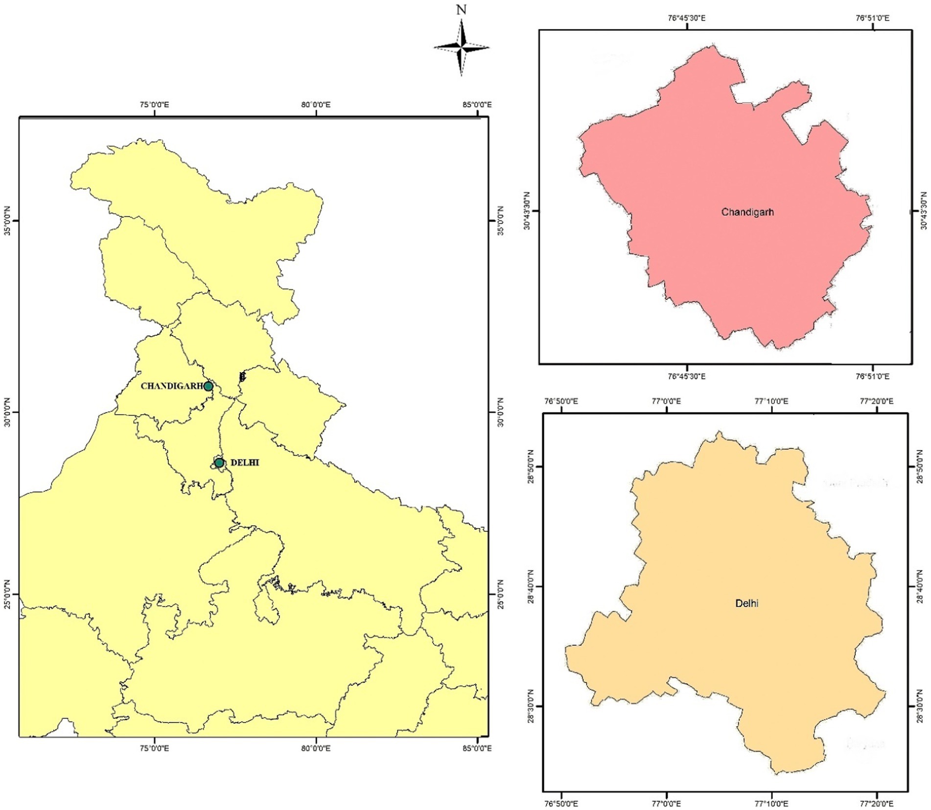
Figure 1. Study area map.

Analytical framework

Different univariate time series techniques were used to capture information from the past and forecast the future. The utilization of these techniques enabled a more efficient understanding of the complex pattern and challenges associated with the forecasting of agricultural commodities.

Autoregressive integrated moving average model

Autoregressive integrated moving average (ARIMA) is a conventional time series model used to estimate and forecast the time series data when they are linear and stationary (Box and Jenkins, 1976). There are three parameters for the ARIMA model: autoregression (p), integration (d), and the moving average (q). The ARIMA model can be expressed as follows:

$\varnothing \left(B\right){\left(1-B\right)}^d{Y}_t=\theta \left(B\right){\epsilon }_t$

$\begin{array}{l}{Y}_t={\varnothing }_1{Y}_t{}_{-1}+{\varnothing }_2{Y}_{t-2}+\cdots +{\varnothing }_p{Y}_{t-p}+{\epsilon }_t\\ -{\theta }_1{\epsilon }_{t-1}-{\theta }_2{\epsilon }_{t-2}-\cdots -{\theta }_q{\epsilon }_{t-q}\end{array}$

where ∅(B) is the autoregressive parameter, θ(B) is the moving average parameter, ɛ_t is the white noise or error term, d is the differencing term, and B is the backshift operator. The major steps involved in building the ARIMA model are:

Identification

The values of p and q can be found based on the number of lagged observations of the dependent variable and the number of lagged errors using the partial autocorrelation function (PACF) plot and autocorrelation function (ACF) plot. The integration (d) indicates the number of times the data is differenced to convert them into stationary (Darekar and Reddy, 2017). Initially, the data must be checked for stationarity using the augmented Dickey–Fuller (ADF) test. If the data are non-stationary, then they must be differenced using appropriate lags to convert them to stationarity.

Parameter estimation

The parameters AR and MA of ARIMA models are estimated using maximum likelihood estimation (MLE). The model which gives the lowest Akaike information criterion (AIC) and Bayesian information criterion (BIC) values are fitted for the data. AIC measures the goodness-of-fit of a statistical model and it is given by

$\mathrm{AIC}=-2\log \left(\mathrm{L}\right)+2\mathrm{k}$

where L is the likelihood function of the model and k is the number of parameters in the model. The AIC penalizes the models that have a large number of parameters relative to the amount of data. The BIC is similar to the AIC but includes a stronger penalty based on model complexity and it is given by

$\mathrm{BIC}=-2\log \left(\mathrm{L}\right)+\mathrm{k}\log \left(\mathrm{n}\right)$

Diagnostics and forecasting

After fitting the model, the residuals are checked for the presence of white noise, i.e., the residuals should be uncorrelated. If the model has white noise, it is taken for forecasting, or else the model is refitted until it attains white noise. The presence of white noise is examined through a quantity Q known as the Box-Pierce statistic (a function of autocorrelations of residuals) whose approximate distribution is chi-square and is computed as follows:

$\mathrm{Q}=\mathrm{n}\Sigma r_{\left(j\right)}^2$

where n is the number of observations in the series and r (j) is the estimated autocorrelation at lag j, extending the summation from 1 to k with k as the maximum positive integer lag. Q follows chi-square with (k˗m˗1) degrees of freedom where m-1 is the number of parameters estimated in the model.

Artificial neural network model

An artificial neural network (ANN) is a computational model inspired by the structure and functionality of biological neural networks. They are a network of interconnected neurons mimicking the function of the human brain. A feedforward neural network (FFNN) is one of the basic neural networks that serve as a non-linear time series model for forecasting purposes (Jha and Sinha, 2013). They are made of input, hidden, and output nodes in which every unit in a particular layer is related to every unit in the previous layer. The data is given through the input node, and the result is obtained from the output node. The in-between hidden layer is the place where processing is done. Each layer consists of weights and biases. The number of input and hidden nodes is determined by experimentation, as there is no theoretical base for finding these parameters. The mathematical representation of the ANN model is given as:

$Y_t={\alpha }_0+{\displaystyle {\sum }_{j=1}^q{\alpha }_{j}g}\left({\beta }_{0j}+{\displaystyle {\sum }_{i=1}^p{\beta }_{ij}{Y}_t{}_{-p}}\right)+{\epsilon }_t$

where 𝛼_𝑗 (𝑗 = 0, 1, 2,…, 𝑞) and 𝛽_𝑖𝑗 (𝑖 = 0, 1, 2,…, 𝑝, 𝑗 = 0, 1, 2,…, 𝑞) are the model parameters, also called as the connection weights, p is the number of input nodes, q is the number of hidden nodes, and 𝑔 is the activation function. The ANN model was applied only after confirming the non-linearity in the datasets. Two major steps are involved in the process of fitting a time series model using an ANN, i.e., choosing the right number of nodes for the input layer (p) and hidden layer (q). The choice of p is critical since it has a significant impact on the non-linear autocorrelation structure (Soumen and Debasis, 2018). The selection of q is also subject to faults that could lead to issues with underfitting and overfitting. Unfortunately, the selection of appropriate nodes for input and output layers does not have any prior procedure, so different combinations of networks are fitted until a suitable model is chosen.

Hybrid time series model

Time series data are complex data structures composed of information in linear or non-linear forms. The hybrid time series model is the combination of different time series techniques which adds the strengths of different techniques to improve the accuracy of forecasting (Rathod et al., 2017). Some of the hybrid techniques employed in the study are given as follows:

ARMA-GARCH

ARMA-GARCH is the combination of an autoregressive moving average (ARMA) with a generalized autoregressive conditional heteroskedasticity (GARCH) model which helps to capture the linear information along with volatile information present in the residuals of the mean model. ARMA is the mean model which helps in modeling the linearity of the time series, while GARCH helps in modeling the volatility or the variance (Bollerslev, 1986). ARMA-GARCH models are specified by four parameters: the orders of the autoregressive process (p) and moving average process (q) for the mean component, and the orders of the autoregressive process (r) and the moving average process (s) for the volatility component.

$\begin{array}{l}Mean\mathrm{}equation\mathrm{}:{\mathrm{Y}}_{\mathrm{t}}={\phi }_1\ast {\mathrm{Y}}_{\mathrm{t}-1}+\dots +{\phi }_{\mathrm{p}}\ast {\mathrm{Y}}_{\mathrm{t}-\mathrm{p}}\\ +{\theta }_1\ast {\mathrm{e}}_{\mathrm{t}-1}+\dots +{\theta }_{\mathrm{q}}\ast {\mathrm{e}}_{\mathrm{t}-\mathrm{q}}\end{array}$

$Variance\mathrm{}equation\mathrm{}:{\sigma }_{\mathrm{t}}{}^2={\alpha }_0+{\alpha }_1\ast {\mathrm{e}}_{\mathrm{t}-1}{}^2+{\beta }_1\ast {\sigma }_{\mathrm{t}-1}{}^2$

where φ₁, φ_p and θ₁, θ_q are the coefficients of the AR and MA terms, e_t is the error term at time t, and σ_t² is the conditional variance of the error term at a time t with non-negative α and β terms. Checking for heteroskedasticity in the squared residuals (Lama et al., 2016) of the mean model is the first and most important step before proceeding with fitting the of volatility model. ARCH-Lagrange Multiplier (LM) test is based on the regressing the squared residuals from a given model onto their lagged values. The null hypothesis of the ARCH-LM test is that there is no ARCH effect in the residuals. The formula for the ARCH-LM test statistic is:

$\mathrm{LM}\mathrm{test}={\mathrm{nR}}^2$

where n is the sample size and R² is the R-squared value from the auxiliary regression of the squared residuals onto their p-lagged values. The GARCH model is fitted only if heteroskedasticity is found in the residuals. AIC and BIC values are used to choose the optimal model.

ARIMA-ANN model

The hybrid time series model with the combination of ARIMA and ANN combines the strengths of both linear and non-linear techniques to improve the accuracy of time series forecasting (Zhang et al., 2015). The general form of hybrid methodology is given by

${\mathrm{y}}_{\mathrm{t}}={\mathrm{L}}_{\mathrm{t}}+{\mathrm{N}}_{\mathrm{t}}$

where L_t and N_t are the linear and non-linear components present in the time series y_t, respectively. First, the ARIMA model is fitted to the data to capture the linear dependencies with the prediction series denoted as $\widehat{\mathrm{L}}$ _t. Second, the residuals (e_t = y_t − $\widehat{L}$ _t) of the ARIMA model are used as inputs to the ANN model. The ANN is trained to learn the non-linear patterns in the residuals that are not captured by the ARIMA model. Finally, the outputs of the ARIMA and ANN models are combined to produce the final forecast values.

${\widehat{\mathrm{y}}}_{\mathrm{t}}={\widehat{\mathrm{L}}}_{\mathrm{t}}+{\widehat{\mathrm{N}}}_{\mathrm{t}}$

where $\widehat{\mathrm{L}}$ _t and $\widehat{\mathrm{N}}$ _t are the forecasted linear and non-linear components. The ANN model is applied to the residuals of ARIMA only after confirming the presence of non-linearity using the Brock–Dechert–Scheinkman (BDS) test (Naveena and Subedar, 2017). This approach offers a robust and effective means of analyzing time series data, combining the abilities of both linear and non-linear models. The working flow chart for the hybrid model is given in Figure 2.

FIGURE 2

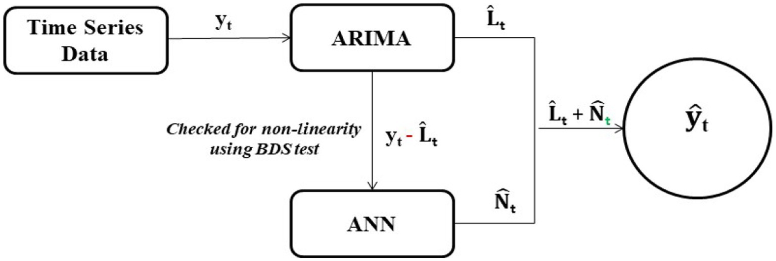
Figure 2. Flowchart for performing hybrid ARIMA-ANN model.

Empirical mode decomposition

Empirical mode decomposition (EMD) is a type of self-adaptive time series decomposition approach used to handle non-stationary and non-linear time series data, especially the arrivals and prices of agricultural commodities. The fundamental idea of EMD is to decompose a signal into a finite number of oscillatory components called intrinsic mode functions (IMFs) with a residual term (Huang et al., 1998). It is a data-driven technique that adaptively extracts the oscillatory modes from the signal based on the local extrema. Each IMF has a unique amplitude and frequency modulation for each set of data. There are two requirements that an IMF must meet: (i) the total number of zero crossings and extreme values in the data series must be equal or differ by not more than one, and (ii) the mean value of the envelope determined by the local maxima and minima must be always zero. Generally, the data are present in the form where fast oscillation signals (Das et al., 2020) are likely superimposed over the slow oscillations, i.e.,

$x\left(t\right)=d_1\left(t\right)+r_1\left(t\right)$

where d(t) = high frequency part, i.e., IMF, and r(t) = low frequency part, i.e., residuals. The EMD algorithm iterates on the slow oscillation component by considering it as a new signal.

${\mathrm{r}}_1\left(t\right)=d_2\left(t\right)+r_2\left(t\right)$

After full decomposition, the data are decomposed into many IMFs and residuals.

$\mathrm{Data}=\mathrm{sum}\mathrm{of\; IMFs}+\mathrm{final\; residue}\mathrm{.}$

The stepwise procedure of the EMD algorithm for the price series x_t is mentioned below:

Step 1: Identify all extrema of x(t).

Step 2: Interpolate the local maxima to form an upper envelope u(x).

Step 3: Interpolate the local minima to form a lower envelope l(x).

Step 4: Calculate the mean envelope: m(t) = $\frac{u\left(x\right)+l\left(x\right)}{2}$

Step 5: Extract the mean from the signal: h(t) = x(t) − m(t)

Step 6: Check whether h(t) satisfies the IMF condition.

• YES: h(t) is an IMF, stop shifting.

• NO: let x(t) = h(t), keep shifting.

However, EMD encounters limitations such as mode mixing and boundary effects, which compromise the accuracy of decomposition (Choudhary et al., 2019). Ensemble empirical mode decomposition (EEMD), an enhanced version of EMD, was developed to address the limitations of EMD. EEMD is an ensemble-based variation of EMD that adds noise to the signal to improve decomposition quality and robustness. This helps to alleviate mode mixing issues by averaging the decompositions and enhances the signal-to-noise ratio that results in providing better decomposition results, especially in the presence of noise. The procedure for performing EEMD is:

• Generate and add a quantity of Gaussian white noises n_t (j) into data series x_t, n_t (j) ~ N (0, σ²)

$x_t\left(\mathrm{j}\right)=x_t+{\mathrm{n}}_t\left(\mathrm{j}\right)$

• Apply EMD to newly formed price series x_t (j) and decompose it into a set of IMFs c_t(ij) and residual r_t (j) where c_t (ij) is j^th (i – 1, 2,…, n) IMF decomposed by EMD after adding the n_t (j) for j^th (j = 1, 2,…, w) time.

• Repeat the above two steps for w times to obtain all IMFs and residuals.

The process of EEMD begins with the decomposition of data into different intrinsic mode functions and a residue. After the decomposition, each IMFs and residue are considered as separate datasets, and the desired time series model is applied like the usual procedure. The fitted and forecasted values of each set are bagged together at the end to get the final fitted and forecasted values. The graphical flowchart of EEMD which employs the ARIMA, ANN, and GARCH models is given in Figure 3.

FIGURE 3

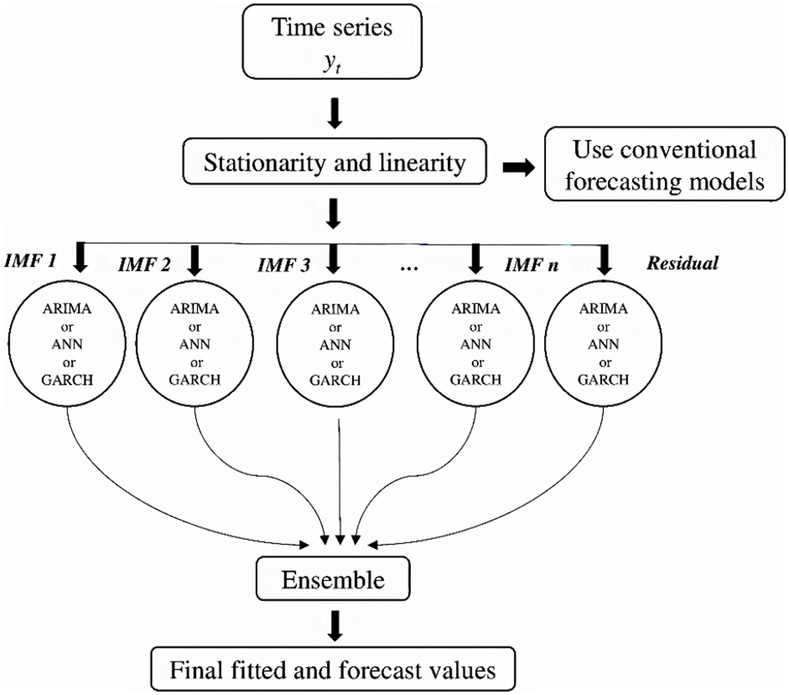
Figure 3. Flowchart for performing hybrid EEMD model.

Performance metrics

Mean absolute percentage error, root mean square percentage error (RMSPE), and mean absolute error (MAE) were employed to find the best-performing time series model for the data.

$\mathrm{MAPE=}\left(\sqrt{{\displaystyle {\sum }_{\mathrm{t=1}}^{\mathrm{n}}|\frac{{\mathrm{Y}}_{\mathrm{t}}-{\widehat{\mathrm{Y}}}_{\mathrm{t}}}{{\mathrm{Y}}_{\mathrm{t}}}{|}^2}/\mathrm{n}}\right)\ast 100$

$\mathrm{RMSPE=}\left(\sqrt{{\displaystyle {\sum }_{\mathrm{t=1}}^{\mathrm{n}}{\left\{\frac{{\mathrm{Y}}_{\mathrm{t}}-{\widehat{\mathrm{Y}}}_{\mathrm{t}}}{{\mathrm{Y}}_{\mathrm{t}}}\right\}}^2}/\mathrm{n}}\right)\ast 100$

$\mathrm{MAE}=\frac{1}{\mathrm{n}}{\displaystyle \sum }_{\mathrm{t}=1}^{\mathrm{n}}\left|{\mathrm{Y}}_{\mathrm{t}}-{\widehat{\mathrm{Y}}}_{\mathrm{t}}\right|$

where Y_𝑡 is the original observation for the period t, $\widehat{Y}$ _𝑡 is the corresponding forecasted value from the fitted model, and n is the number of observations.

Results and discussion

The data analysis conducted in this study revealed notable disparities between the two markets in terms of the average arrivals and prices, as depicted in Table 1. The data exhibited a positive skewness, with mean arrivals of 2,468.25 MT and 24,208.81 MT in the Chandigarh and Delhi markets, respectively. Correspondingly, the mean wholesale prices were recorded as 1,419.76 (Rs./Qtl) and 1,514.92 (Rs./Qtl) for the respective markets. The Cuddy Della Valle Index (CDVI) was employed to assess the volatility around the trend of time series data (Dudhat et al., 2017), while the coefficient of variation (CV) was utilized to capture deviations from the mean. The CDVI indicated a substantial level of instability in both arrivals and prices, with the exception of the Delhi market, which exhibited a moderate instability index (Sinha et al., 2018). These findings were further supported by the CV results. The arrivals in Chandigarh and Delhi markets showed a positive compound growth rate (CGR) of 10.95 and 3.82%, respectively. Similarly, the growth rates for prices were observed as 8.34 and 7.79%, respectively (Agarwal et al., 2018). Figure 4 displays the time series graphs for the data, illustrating the non-linear and non-stationary nature of the arrivals and prices in both markets, with several breakpoints observed over the years. The typical behavior of agricultural commodities was further confirmed in onion data by conducting the BDS test, autocorrelation (AC) test, and ADF test (Table 2). The BDS test conducted at different embedding dimensions confirmed the non-linearity in data with statistical significance (Saha et al., 2020). The data were found to be autocorrelated with a value of p of 0.00. The ADF test showed that the data were non-stationary at levels and were converted to stationary after the first differencing. These preliminary tests provided the necessary foundation for the application of subsequent time series techniques to the dataset.

TABLE 1

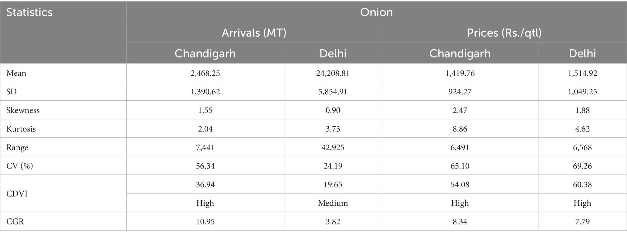
Table 1. Descriptive statistics on the arrivals and prices of onion.

FIGURE 4

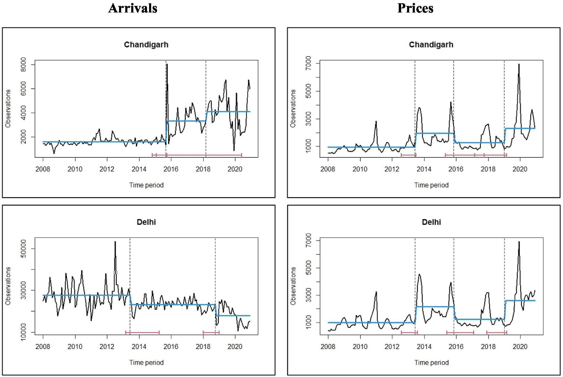
Figure 4. Time series plots of arrivals and prices of onion along with structural breakpoints.

TABLE 2

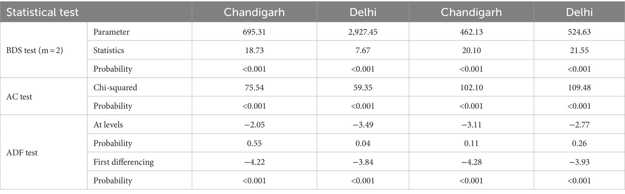
Table 2. Prerequisites test for time series data.

ARIMA model

Table 3 presents the outcomes of the linear models that best fit the data. For the arrivals of Chandigarh and Delhi markets, the best-fitted models were found to be ARIMA (0,1,1) and ARIMA (1,1,1), respectively, based on their low values of AIC and BIC. Likewise, the prices in both markets were modeled using ARIMA (1,1,2) and ARIMA (2,1,1) (Mishra et al., 2013). All the parameters of the ARIMA model were found to be statistically significant with a value of p of 0.01. Results of the Box-Pierce (BP) test indicated that all the fitted models were white noise. However, the Arch-LM test revealed the presence of heteroskedasticity (Jalikatti and Patil, 2015) only in the residuals of the ARIMA models of the price series. Therefore, to model the price series, a GARCH model was employed while the ARIMA model was used solely for comparative purposes, despite the non-linear nature of the data.

TABLE 3

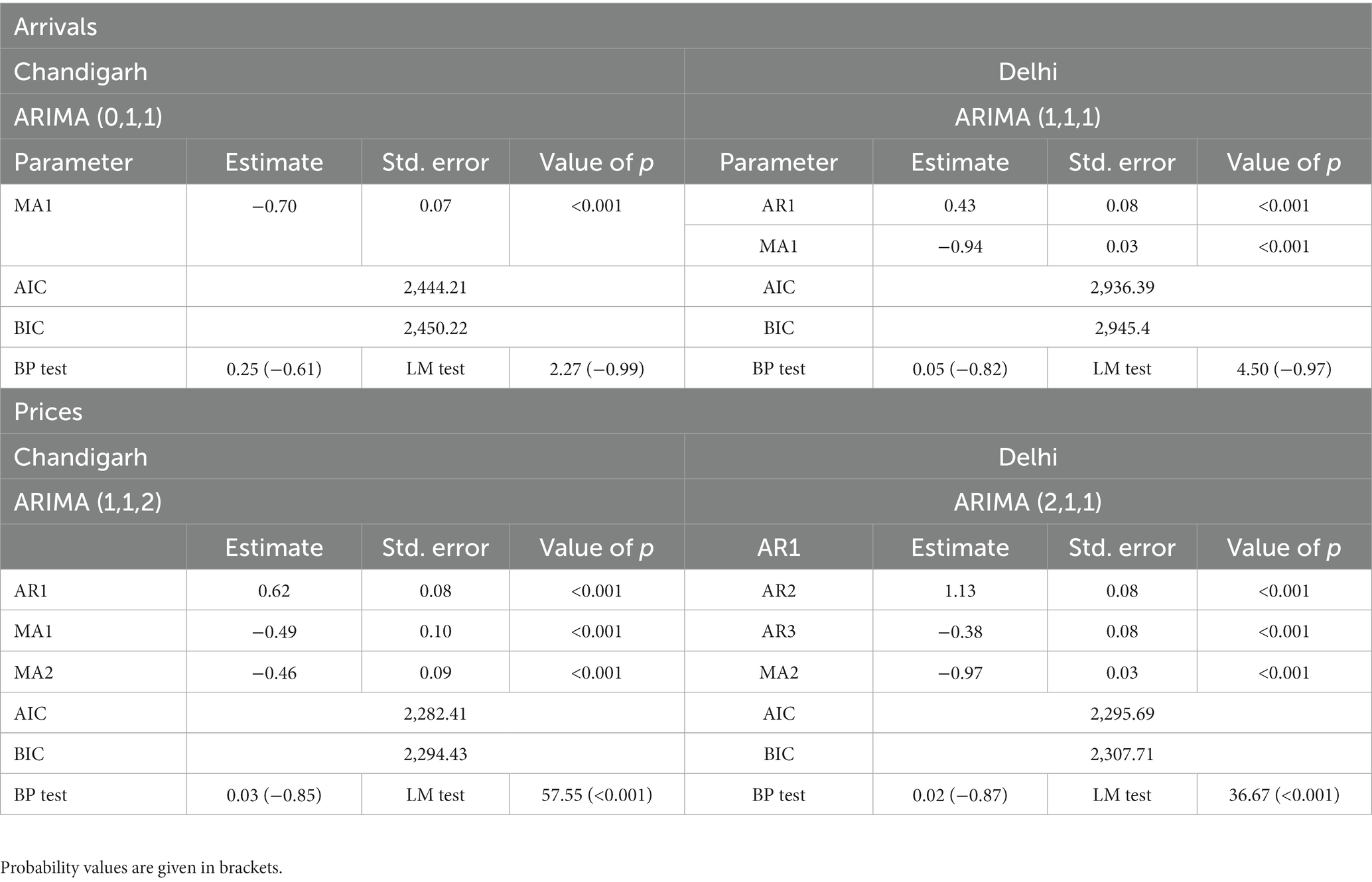
Table 3. Estimates of parameters of the ARIMA model.

ARMA-GARCH model

The outcomes of the ARMA-GARCH model are presented in Table 4. The models ARMA (1,2) + GARCH (2,1) and ARMA (2,1) + GARCH (2,1) were found to be the best fit based on their AIC and BIC values. Low AIC and BIC values were found of 14.66 and 14.82 for onion prices in Chandigarh and 14.68 and 14.85 for prices in Delhi, respectively (Bawa et al., 2021). Both the series were fitted with the GARCH (2,1) model, i.e., α1, α2, and β1. The lags mean model were considered from the ARIMA model. The mean value of both the models along with omega and alpha1 of Delhi markets were statistically significant with a value of p of 0.01, whereas the rest of the mean and volatility parameters were non-significant (Ghosh et al., 2020).

TABLE 4

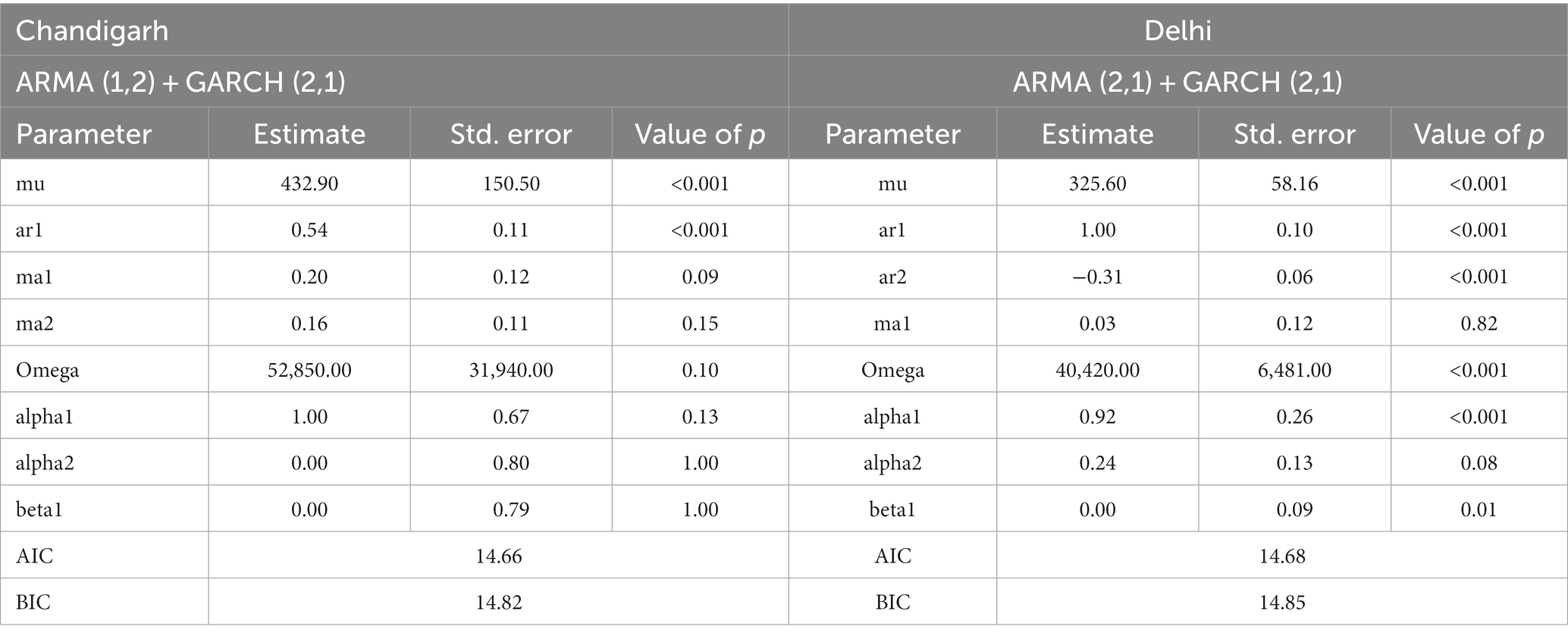
Table 4. Parameter estimation of the ARIMA-GARCH model.

ANN model

Considering the confirmation of non-linearity in the arrivals and prices through the BDS test from Table 2, the application of ANN was more justifiable. The FFNN was employed to build the ANN network for the data with a sigmoid activation function (Nelson et al., 1999). Various combinations of input and output nodes were tested for the data with a minimum of 25 iterations to identify the optimal network configuration. Table 5 shows the results of the ANN model with the final network selected. For the arrival series, 3–2-1 and 3–11–1 networks were fitted while 2–2-1 and 2–2-1 networks were fitted for the price series of Chandigarh and Delhi markets, respectively. Notably, the onion arrivals at the Delhi market required more lags in the hidden node (Jha and Sinha, 2014). The results of the BP test confirmed the adequacy of the fitted ANN model.

TABLE 5

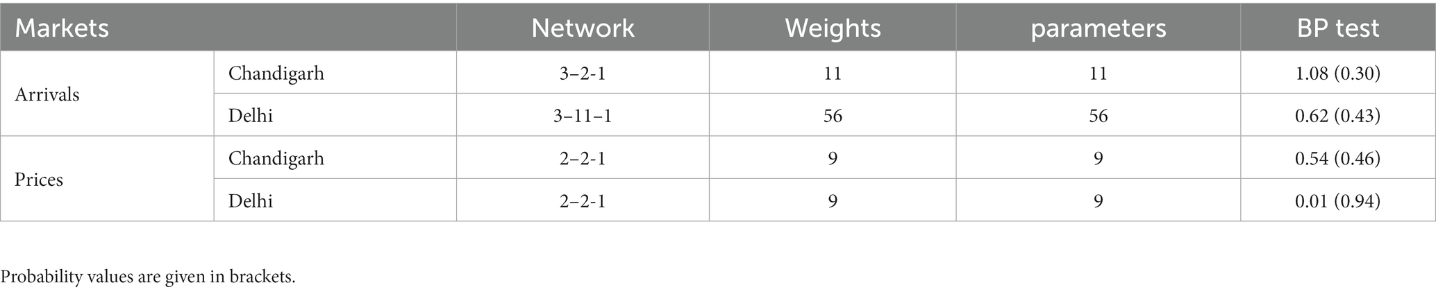
Table 5. Parameter estimation of the ANN model.

ARIMA-ANN

The initial step involved performing the BDS test on the residuals derived from the applied ARIMA model, aiming to detect the presence of non-linearity. The results of the BDS test indicated that all residuals from the fitted ARIMA model exhibited unexplained non-linear characteristics, as evidenced by a statistically significant value of p of 0.01 (Table 6). In order to address this issue, the ANN model was employed to capture the non-linear patterns present in the residuals. The ANN model was configured with appropriate lag lengths for both the input and hidden nodes (Alam et al., 2018). The findings revealed that 6–11–1 and 10–1-1 were the best networks fitted for the arrivals, while the 7–4-1 and 8–4-1 networks were fitted to the price series of Chandigarh and Delhi markets, respectively (Zhang, 2003). Furthermore, the adequacy of the fitted models was confirmed by the value of ps obtained from the BP test. Table 7 represents the weights and parameters utilized in fitting the networks.

TABLE 6

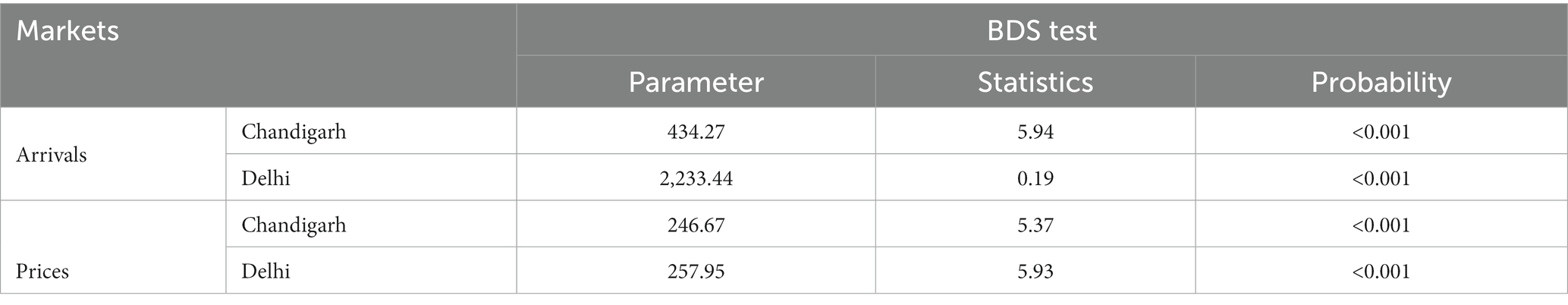
Table 6. Results of BDS test on residuals of ARIMA model.

TABLE 7

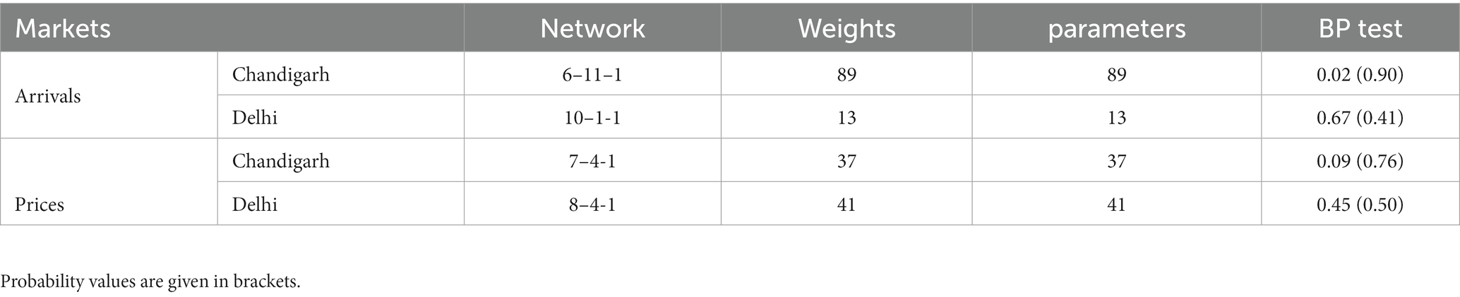
Table 7. Results of ANN model on residuals of ARIMA model.

Ensemble empirical mode decomposition-based time series models

To ensure the suitability of the data for analysis, the application of EEMD techniques was contingent upon verifying the presence of non-linearity and non-stationarity. Following confirmation through the BDS test and ADF test, the arrivals and price data of onions at the Chandigarh and Delhi markets were decomposed using EEMD. Through the decomposition process, the raw datasets were effectively separated into six intrinsic mode functions (IMFs) and one residual component. This decomposition was visually depicted in Figure 5. It was observed that the decomposed IMFs exhibited a pattern characterized by decreasing fluctuations and increasing amplitude (Guo et al., 2012). Subsequently, time series models such as ARIMA, ANN, and GARCH were individually fitted to each IMF and the residual component using the usual procedures (Wu and Huang, 2009). For every IMF and the residual component, fitted and forecasted values were calculated. Finally, all the fitted and forecasted values obtained from the IMFs and the residual were combined, resulting in a unified output. This process involved aggregating the individual values generated for each IMF and the residual, allowing for a comprehensive and consolidated analysis of the data.

FIGURE 5

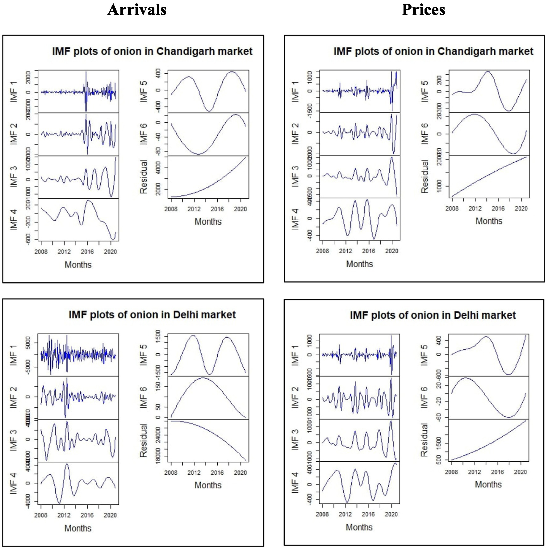
Figure 5. IMFs and residuals of arrivals and prices of onion decomposed using EMD.

Selection of best-fitting model

In order to evaluate the accuracy of the fitted models, a range of error metrics, including mean absolute percentage error (MAPE), root mean percentage squared error (RMPSE), and mean absolute error (MAE), were employed. Table 8 presents the results of these metrics for the different models. It was observed that the EEMD-ARIMA model exhibited the best fit for the arrival series of Chandigarh, while the EEMD-ANN model performed well for the remaining data (Choudhury et al., 2019). The MAPE values for the best-fitted models were found to be 17.74 and 6.78% for the arrival series and 9.76 and 10.24% for the price series of Chandigarh and Delhi, respectively. Overall, the findings suggest that the EEBD-ANN and EEBD-ARIMA models (Fang et al., 2020), followed by the ANN model, were the most effective in forecasting both the arrival and price series. Interestingly, the GARCH model, which is typically known for its efficiency in handling volatile data, did not perform well for the dataset under study. Consequently, the arrival and price series were forecasted based on the best-fitted models. Figure 6 illustrates the forecasted values (Wang et al., 2017) of the entire dataset using the respective best-fitted models.

TABLE 8

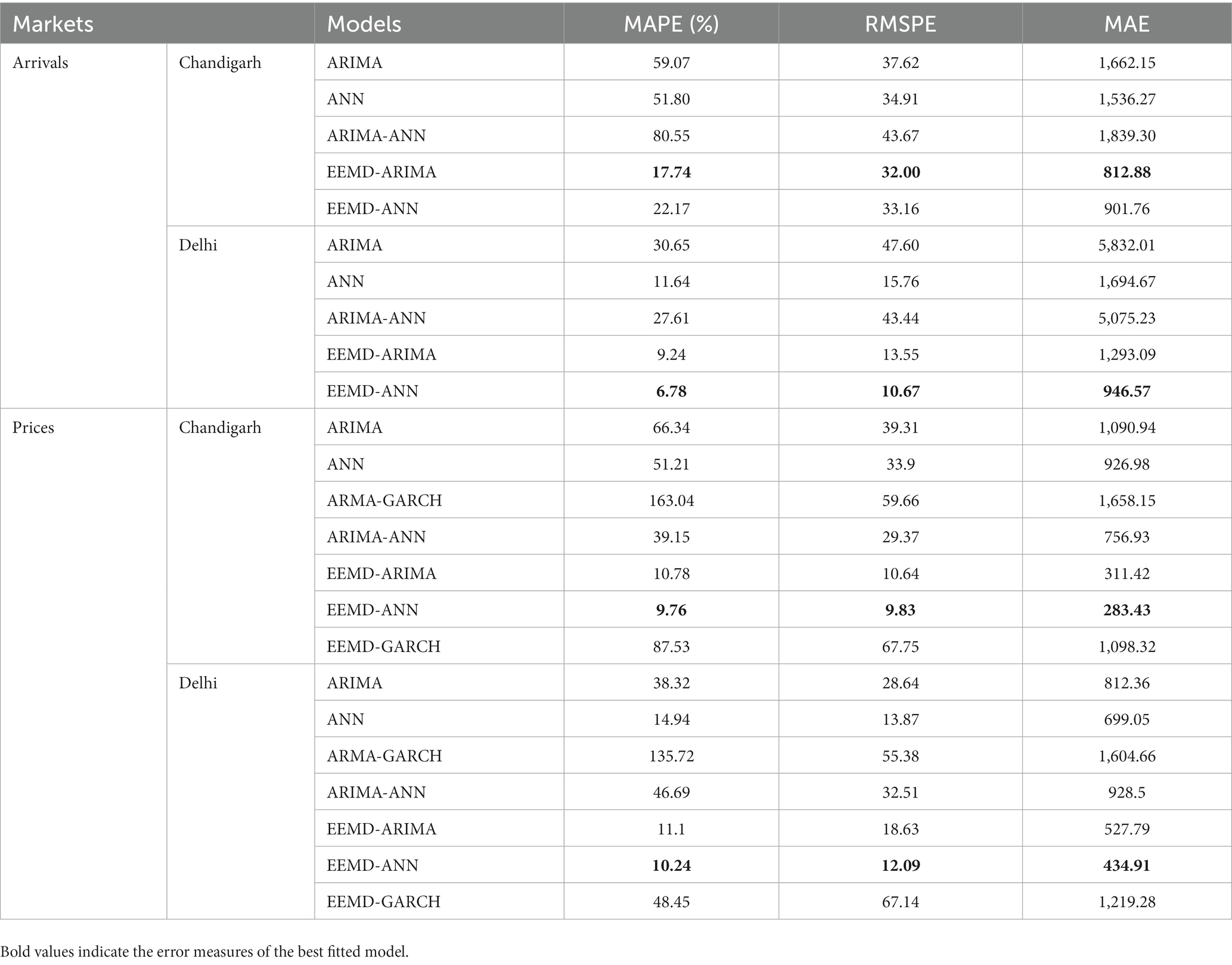
Table 8. Performance metric of fitted models.

FIGURE 6

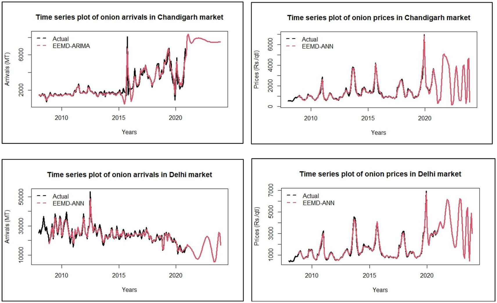
Figure 6. Forecasting plots for arrivals and prices of onion using the best-fitted model.

General discussion

Despite being major urban centers in Northern India, cities like Chandigarh and Delhi face challenges in achieving self-sustainability in agricultural production. These cities rely heavily on neighboring regions for the supply of commodities, including onions which can be prominently observed from the previous studies (Mishra et al., 2013; Jalikatti and Patil, 2015; Sinha et al., 2018; Dahiya, 2022; Garai et al., 2023). As a result, they depend on transportation from hub areas, which adds additional costs to the procurement of vegetables. The time series plot showed many breakpoints which indicates the irregular variation in the arrivals and prices pattern of onions. The more the fluctuation in the trends, the more the volatility which results in an unstable supply and prices (Saha et al., 2020). These variations may be induced by natural calamities like drought, famine, and flood. The implication of policy related to agriculture would also cause such an impact on the pattern of onions. Different kinds of machine learning models are employed to figure out the volatility in onions (Babu and Mallikharjuna, 2022). The present study attempts to employ all these techniques additionally with ensemble techniques. The ensemble techniques combined with the machine learning models were found to perform better for the data. The outperformance of decomposition techniques over the other models is eventual evidence of the presence of complexity in the data which was further supported by the results of Table 2. The forecasting graphs also showed the incidence of volatility especially in prices. Thus, the volatile nature of onion was further confirmed by the results of the study. The government should provide proper guidance and support to onion cultivators regarding the fluctuation phenomena. Proper forecasting should be done every year so that the farmers can give considerable attention to onion cultivation and marketing. It could also help the government to optimally manage fund allocations for the agricultural sector. As there is no minimum support price (MSP) for vegetables, the government should find possible options to avail MSP for volatile crops, especially onions. This study would help in framing the optimum MSP and other beneficial policies for onion as suggested by previous studies (Babu and Mallikharjuna, 2022). The government should take strict actions against the middlemen who are involved in hedging and hoarding practices that artificially create fluctuations in the markets.

Conclusion

The study evaluates the performance of different forecasting models like ARIMA and ANN, hybrid models like ARMA-GARCH and ARIMA-ANN, and decomposition models like EEMD-ARIMA and EEMD-ANN over multifaceted data. The results of the summary statistics on the arrivals and prices of onion at Chandigarh and Delhi markets showed that the mean arrivals and mean prices were high at Delhi markets, viz., 24,208.81 MT and 1,514.93 Rs./Qtl. The time series plot showed many structural breaks in the data over the years which were due to a high instability index. The arrivals of onions at Delhi markets were observed with a medium instability index. The preliminary test confirmed that data used for the study were autocorrelated, non-linear, and non-stationary at levels with positive growth rates over the years. Therefore, forecasting these unpredictable agricultural arrivals and prices would be helpful for the farmers, stakeholders, and governmental bodies for better planning in the future. From the results of the study, it was found that the ANN model does not consider the stationarity condition but is good at handling non-linearity in data, whereas the ARIMA model can be applied only when the data are stationary and linear. These limitations are overcome by applying EEMD techniques which can analyze the data with both the issues and explain the different levels of fluctuations using the intrinsic mode function. The overall results conclude that EEMD-ANN and EEMD-ARIMA were the best performing models for the study data and had less error rate which were observed using the error metrics like MAPE, RMSPE and MAE. The data were forecasted for the next 3 years using decomposition techniques. All the extracted information from this study could help in better decision-making regarding the production, marketing, and policymaking on the arrivals and prices of onion.

Thus, the attempts to highlight the problems of instability in the arrivals and prices of onion at Chandigarh and Delhi markets through different statistical measures were shown in this study. Additionally, the performance of different time series models was examined, and the best-performing model was chosen to forecast the future pattern of arrivals and price of onions in study markets. In the future, the accuracy of forecasting can be further improved by accounting for weather parameters, as they are one of the prime factors influencing the patterns of agricultural commodities.

Data availability statement

The datasets presented in this study can be found in online repositories. The names of the repository/repositories and accession number(s) can be found at: https://www.nhb.gov.in/OnlineClient/MonthlyPriceAndArrivalReport.aspx.

Author contributions

All authors listed have made a substantial, direct, and intellectual contribution to the work and approved it for publication.

Conflict of interest

The authors declare that the research was conducted in the absence of any commercial or financial relationships that could be construed as a potential conflict of interest.

The reviewer AK declared a shared affiliation with the author AA to the handling editor at the time of review.

Publisher’s note

All claims expressed in this article are solely those of the authors and do not necessarily represent those of their affiliated organizations, or those of the publisher, the editors and the reviewers. Any product that may be evaluated in this article, or claim that may be made by its manufacturer, is not guaranteed or endorsed by the publisher.

References

Agarwal, P., Singh, R., and Singh, O. P. (2018). Dynamics of prices and arrivals of major vegetables: a case of Haldwani and Dehradun markets, Uttarakhand. J. Agric. Dev. Policy 28:1.

Google Scholar

Alam, W., Sinha, K. A., Kumar, R. R., Ray, M. R., Rathod, S. A., Singh, K. N., et al. (2018). Hybrid linear time series approach for long term forecasting of crop yield. Indian J. Agric. Sci. 88, 1275–1279. doi: 10.56093/ijas.v88i8.82573

CrossRef Full Text | Google Scholar

Allen, P. G. (1994). Economic forecasting in agriculture. Int. J. Forecast. 10, 81–135. doi: 10.1016/0169-2070(94)90052-3

CrossRef Full Text | Google Scholar

Anjoy, P., Paul, R. K., Sinha, K., Paul, A. K., and Ray, M. (2017). A hybrid wavelet based neural networks model for predicting monthly WPI of pulses in India. Indian J. Agric. Sci. 87, 834–839. doi: 10.56093/ijas.v87i6.71022

CrossRef Full Text | Google Scholar

Areef, M., Rajeswari, S., Vani, N., and Naidu, G. M. (2020). Price behaviour and forecasting of onion prices in Kurnool market, Andhra Pradesh State. Econ. Aff. 65, 43–50. doi: 10.30954/0424-2513.1.2020.6

CrossRef Full Text | Google Scholar

Arjun, K. M. (2013). Indian agriculture-status, importance and role in Indian economy. Int. J. Agric. Food Sci. Technol. 4, 343–346.

Google Scholar

Babu, K. S., and Mallikharjuna, R. K. (2022). Onion Price prediction using machine learning approaches. In Proceedings of International Conference on Computational Intelligence and Data Engineering: ICCIDE 2021. Singapore: Springer Nature Singapore, pp. 175–189

Google Scholar

Bawa, M. U., Dikko, H. G., Shabri, A., Garba, J., and Sadiku, S. (2021). Forecasting performance of hybrid ARIMA-FIGARCH model and hybrid of ARIMA-GARCH model: a comparative study. J. Math. Prob. Equ. Stat. 2, 48–58.

Google Scholar

Bollerslev, T. (1986). Generalized autoregressive conditional heteroskedasticity. J. Econ. 31, 307–327. doi: 10.1016/0304-4076(86)90063-1

CrossRef Full Text | Google Scholar

Box, G. E., and Jenkins, G. M. (1976). Time series analysis, control, and forecasting. San Francisco, CA: Holden Day, p. 10.

Google Scholar

Choudhary, K. A., Jha, G. K., Kumar, R. R., and Mishra, D. C. (2019). Agricultural commodity price analysis using ensemble empirical mode decomposition: a case study of daily potato price series. Indian J. Agric. Sci. 89, 882–886. doi: 10.56093/ijas.v89i5.89682

CrossRef Full Text | Google Scholar

Choudhury, K., Jha, G. K., Das, P., and Chaturvedi, K. K. (2019). Forecasting potato price using ensemble artificial neural networks. Indian J. Ext. Educ. 55, 73–77.

Google Scholar

Dahiya, P. (2022). Modeling and forecasting of all India monthly average wholesale Price volatility of onion: an application of GARCH and EGARCH techniques. Curr. J. Appl. Sci. Technol. 41, 91–100.

Google Scholar

Darekar, A., and Reddy, A. (2017). Predicting market price of soybean in major India studies through ARIMA model. J. Food Legum. 30, 73–76. doi: 10.2139/ssrn.3089035

CrossRef Full Text | Google Scholar

Das, P., Jha, G. K., and Lama, A. (2023). Empirical mode decomposition based ensemble hybrid machine learning models for agricultural commodity Price forecasting, No. 21. pp. 99–112.

Google Scholar

Das, P., Jha, G. K., Lama, A., Parsad, R., and Mishra, D. (2020). Empirical mode decomposition based support vector regression for agricultural price forecasting. Indian J. Ext. Educ. 56, 7–12.

Google Scholar

Dudhat, A. S., Yadav, P., and Venujayakanth, B. (2017). A statistical analysis on instability and seasonal component in the price series of major domestic groundnut markets in India. Int. J. Curr. Microbiol. Appl. Sci. 6, 815–823. doi: 10.20546/ijcmas.2017.611.096

CrossRef Full Text | Google Scholar

Fang, Y., Guan, B., Wu, S., and Heravi, S. (2020). Optimal forecast combination based on ensemble empirical mode decomposition for agricultural commodity futures prices. J. Forecast. 39, 877–886. doi: 10.1002/for.2665

CrossRef Full Text | Google Scholar

Garai, S., Paul, R. K., Rakshit, D., Yeasin, M., Emam, W., Tashkandy, Y., et al. (2023). Wavelets in combination with stochastic and machine learning models to predict agricultural prices. Mathematics 11:2896. doi: 10.3390/math11132896

CrossRef Full Text | Google Scholar

Ghani, I. M., and Rahim, H. A. (2019) Modeling and forecasting of volatility using ARMA-GARCH: Case study on Malaysia natural rubber prices. In IOP Conference Series: Materials Science and Engineering, Vol. 548. p. 012023.

Google Scholar

Ghosh, S., Singh, K. N., Thangasamy, A., Datta, D., and Lama, A. (2020). Forecasting of onion (Allium cepa) price and volatility movements using ARIMAX-GARCH and DCC models. Indian J. Agric. Sci. 90, 1009–1013. doi: 10.56093/ijas.v90i5.104384

CrossRef Full Text | Google Scholar

Guo, Z., Zhao, W., Lu, H., and Wang, J. (2012). Multi-step forecasting for wind speed using a modified EMD-based artificial neural network model. Renew. Energy 37, 241–249. doi: 10.1016/j.renene.2011.06.023

CrossRef Full Text | Google Scholar

Huang, N. E., Shen, Z., Long, S. R., Wu, M. C., Shih, H. H., Zheng, Q., et al. (1998). The empirical mode decomposition and the Hilbert spectrum for nonlinear and non-stationary time series analysis. Proc. R. Soc. London A Math. Phys. Eng. Sci. 454, 903–995. doi: 10.1098/rspa.1998.0193

CrossRef Full Text | Google Scholar

Jalikatti, V. N., and Patil, B. L. (2015). Onion price forecasting in Hubli market of northern Karnataka using ARIMA technique. Karnataka J. Agric. Sci. 28, 228–231.

Google Scholar

Jha, G. K., and Sinha, K. (2013). Agricultural price forecasting using neural network model: an innovative information delivery system. Agric. Econ. Res. Rev. 26, 229–239.

Google Scholar

Jha, G. K., and Sinha, K. (2014). Time-delay neural networks for time series prediction: an application to the monthly wholesale price of oilseeds in India. Neural Comput. Appl. 24, 563–571. doi: 10.1007/s00521-012-1264-z

CrossRef Full Text | Google Scholar

Kumar, P., Badal, P. S., Paul, R. K., Jha, G. K., Venkatesh, P., Anbukani, P., et al. (2021). Forecasting onion price for Varanasi market of Uttar Pradesh, India. Agric. Res. 91, 249–253. doi: 10.56093/ijas.v91i2.111603

CrossRef Full Text | Google Scholar

Kumar, M., Shaikh, A. S., and Sharma, R. K. (2022). Market integration and Price transmission analysis of onion in wholesale Markets of India. Asian J. Agric. Exten. Econ. Sociol. 40, 164–171. doi: 10.9734/ajaees/2022/v40i121778

CrossRef Full Text | Google Scholar

Kumar, M., and Thenmozhi, M. (2014). Forecasting stock index returns using ARIMA-SVM, ARIMA-ANN, and ARIMA-random forest hybrid models. Int. J. Bank. Account. Financ. 5, 284–308. doi: 10.1504/IJBAAF.2014.064307

CrossRef Full Text | Google Scholar

Lama, A., Jha, G. K., Gurung, B., Paul, R. K., Bharadwaj, A., and Parsad, R. (2016). A comparative study on time-delay neural network and GARCH models for forecasting agricultural commodity price volatility. J. Indian Soc. Agric. Stat. 70, 7–18.

Google Scholar

Mishra, P., Sarkar, C., Vishwajith, K. P., Dhekale, B. S., and Sahu, P. K. (2013). Instability and forecasting using ARIMA model in area, production and productivity of onion in India. J. Crop Weed 9, 96–101.

Google Scholar

Naveena, K., and Subedar, S. (2017). Hybrid time series modelling for forecasting the price of washed coffee (Arabica plantation coffee) in India. Int. J. Agric. Sci. 9, 975–3710.

Google Scholar

Nelson, M., Hill, T., Remus, W., and O'Connor, M. (1999). Time series forecasting using neural networks: should the data be deseasonalized first? J. Forecast. 18, 359–367. doi: 10.1002/(SICI)1099-131X(199909)18:5<359::AID-FOR746>3.0.CO;2-P

CrossRef Full Text | Google Scholar

Pardhi, R., Singh, R., and Paul, R. K. (2018). Price forecasting of mango in Lucknow market of Uttar Pradesh. Int. J. Agric. Environ. Biotechnol. 11, 357–363.

Google Scholar

Paul, R. K., Bhardwaj, S. P., Singh, D. R., Kumar, A., Arya, P., and Singh, K. N. (2015). Price volatility in food Commodities in India-an Empirical Investigation. Int. J. Agric. Stat. Sci. 11, 395–401.

Google Scholar

Paul, R. K., Das, T., and Yeasin, M. (2023). Ensemble of time series and machine learning model for forecasting volatility in agricultural prices. Natl. Acad. Sci. Lett. 46, 185–188. doi: 10.1007/s40009-023-01218-x

CrossRef Full Text | Google Scholar

Rakshit, D., Paul, R. K., and Panwar, S. (2021). Asymmetric Price volatility of onion in India. Indian J. Agric. Econ. 76, 245–260.

Google Scholar

Rathod, S., Mishra, G. C., and Singh, K. N. (2017). Hybrid time series models for forecasting banana production in Karnataka state, India. J. Indian Soc. Agric. Stat. 71, 193–200.

Google Scholar

Saha, N., Kar, A., Jha, G. K., Kumar, P., Venkatesh, P., and Kumar, R. R. (2020). Forecasting of onion Price in Lasalgaon market and potato Price in Agra market. J. Commun. Mob. Sustain. Dev. 15, 460–466. doi: 10.5958/2231-6736.2020.00029

CrossRef Full Text | Google Scholar

Saha, A., Singh, K. N., Ray, M., and Rathod, S. (2020). A hybrid spatio-temporal modelling: an application to space-time rainfall forecasting. Theor. Appl. Climatol. 142, 1271–1282. doi: 10.1007/s00704-020-03374-2

CrossRef Full Text | Google Scholar

Saxena, R., Singh, N. P., Paul, R. K., and Kumar, R. (2019). Market linkages for the major onion markets in India. Indian J. Hortic. 76, 133–140. doi: 10.5958/0974-0112.2019.00019.7

CrossRef Full Text | Google Scholar

Singh, R. K. (2008). Artificial neural network methodology for modelling and forecasting maize crop yield. Agric. Econ. Res. Rev. 21, 5–10.

Google Scholar

Sinha, K. (2023). “The Price of onions” in The future of India's rural markets: A transformational opportunity. ed. B. S. Sergi (Bingley, England: Emerald Publishing Limited), 49–51.

Google Scholar

Sinha, K., Panwar, S., Alam, W., Singh, K. N., Gurung, B., Paul, R. K., et al. (2018). Price volatility spillover of Indian onion markets: a comparative study. Indian J. Agric. Sci. 88, 114–120.

Google Scholar

Soumen, P., and Debasis, M. (2018). Forecasting monthly rainfall using artificial neural network. RASHI 3, 65–73.

Google Scholar

Sujay, R., Parvati, V. K., Biradar, S. R., Kerur, V. V., and Huilgol, S. S. (2022). Forecasting of onion prices. In Contemporary issues in communication, cloud and big data analytics: Proceedings of CCB 2020 2022. Springer: Singapore, pp. 339–343

Google Scholar

Wang, H., Liu, L., Qian, Z., Wei, H., and Dong, S. (2014). Empirical mode decomposition–autoregressive integrated moving average: hybrid short-term traffic speed prediction model. Transp. Res. Rec. 2460, 66–76. doi: 10.3141/2460-08

CrossRef Full Text | Google Scholar

Wang, D., Yue, C., Wei, S., and Lv, J. (2017). Performance analysis of four decomposition-ensemble models for one-day-ahead agricultural commodity futures price forecasting. Algorithms 10:108. doi: 10.3390/a10030108

CrossRef Full Text | Google Scholar

Wu, Z., and Huang, N. E. (2009). Ensemble empirical mode decomposition: a noise-assisted data analysis method. Adv. Adapt. Data Anal. 01, 1–41. doi: 10.1142/S1793536909000047

CrossRef Full Text | Google Scholar

Zhang, G. P. (2003). Time series forecasting using a hybrid ARIMA and neural network model. Neurocomputing 50, 159–175. doi: 10.1016/S0925-2312(01)00702-0

CrossRef Full Text | Google Scholar

Zhang, J. L., Zhang, Y. J., and Zhang, L. (2015). A novel hybrid method for crude oil price forecasting. Energy Econ. 49, 649–659. doi: 10.1016/j.eneco.2015.02.018

CrossRef Full Text | Google Scholar