An open-source tool for improving on-farm yield forecasting systems

Introduction: The increased frequency of extreme climate events, many of them of rapid onset, observed in many world regions, demands the development of a crop forecasting system for hazard preparedness based on both intraseasonal and extended climate prediction. This paper presents a Fortran version of the Crop Productivity Model AquaCrop that assesses climate and soil fertility effects on yield gap, which is crucial in crop forecasting systems

Methods: Firstly, the Fortran version model - AQF outputs were compared to the latest version of AquaCrop v 6.1. The computational performance of both versions was then compared using a 100-year hypothetical experiment. Then, field experiments combining fertility and water stress on productivity were used to assess AQF model simulation. Finally, we demonstrated the applicability of this software in a crop operational forecast system.

Results: Results revealed that the Fortran version showed statistically similar results to the original version (r² > 0.93 and RMSEn < 11%, except in one experiment) and better computational efficiency. Field data indicated that AQF simulations are in close agreement with observation.

Conclusion: AQF offers a version of the AquaCrop developed for time-consuming applications, such as crop forecast systems and climate change simulations over large areas and explores mitigation and adaptation actions in the face of adverse effects of future climate change.

1. Introduction

The need to assess the adverse effects of extreme climate events on crop productivity and the urge for planning mitigation and adaptation actions has promoted the development of crop forecast systems (Bento et al., 2022; Chitsiko et al., 2022; Dhakar et al., 2022).

Although previous studies have demonstrated the feasibility of a crop forecast system based on the coupling of climate and crop models, few systems have been implemented in an operational mode worldwide, and none in the case of Brazil. For instance, the MARS-crop yield forecasting system - MCYFS, which has been used to monitor crop growth development, evaluate short-term effects of adverse weather events, and provide monthly forecasts of crop yield and production for various crops in the European Union (see Van der Velde and Nisini, 2018; MCYFS, 2022). Another initiative for assessing crop conditions for global markets is GEOGLAM – Crop Monitor for the Agricultural Monitoring Information System- AMIS (Ministerial Declaration, 2011; Becker-Reshef et al., 2019). It encompasses some large producer areas in Brazil but focuses on large-scale agriculture and not smallholder farming.

Several crop simulation models are available in the literature. Among them, it is worth mentioning the APSIM (Holzworth et al., 2018), DSSAT (Hoogenboom et al., 2019), WOFOST (de Wit et al., 2018), and the AquaCrop model (Raes et al., 2009; Steduto et al., 2009). In the case of AquaCrop, the model was designed to simplify the complex processes involved in crop development to facilitate its use in regions with scarce information. Because of this, AquaCrop has been used in many applications worldwide for supporting agriculture practices and research studies involving irrigation (Geerts and Raes, 2009) and sowing management (Abrha et al., 2012); to support farming economic models (García-Vila and Fereres, 2012); seasonal crop forecasts (Bussay et al., 2015; Martins et al., 2018); climate change impacts (van Oort and Zwart, 2017; Martins et al., 2019); food security (Muluneh et al., 2016); irrigation and fertilizer assessment (Shrestha, 2014; Akumaga et al., 2017; Guo et al., 2019; Ranjbar et al., 2019); among many others (Pirmoradian and Davatgar, 2019; Sandhu and Irmak, 2019; Chibarabada et al., 2020; de Roos et al., 2020).

AquaCrop is a freeware package¹, running in a graphical user interface – GUI hereafter denoted “AquaCrop GUI.” Since simulations of AquaCrop GUI are limited to a single field location, a plug-in version of the software is also available, allowing multiple site simulations. Both versions (plug-in and standalone) are available as executable files that cannot be modified for specific applications.

However, an operational crop forecast system requires manipulating and processing large amounts of detailed atmospheric forecasts, high time-spatial resolution imagery, and ground information. Regional climate model outputs are generally provided in specific formats (such as NetCDF - Network Common Data Form which is specific for array-oriented scientific data), which is not compatible with the graphical interface codes of AquaCrop GUI, despite its user-friendly and didactic character. With the increased frequency of drought, often accompanied by rapid intensification linked to evaporative demand- a phenomenon known as ‘flash drought’ (Otkin et al., 2017) - both under current climate conditions (Christian et al., 2021) and projected future climate change (Vijay and Srinivas, 2022), it becomes evident that there is an urgent need for new tools. These tools can assist in timely decision-making on intraseasonal or seasonal climate scales, as well as aid in designing adaptation strategies to address future climate change.

Considering those limitations, this study aims to present an open-source crop forecast model based on the AquaCrop, denoted as AquaCrop Fortran (AQF). The software includes the soil fertility module based on the AquaCrop GUI module (van Gaelen et al., 2014; Raes et al., 2018), enabling the estimation of actual (on-farm) yield in applications where the yield gap accounting is relevant.

Several tests were performed to compare the outputs of AQF and AquaCrop GUI. We also compared AQF against field observations to prove the capability and flexibility of the fertility module, both in controlled and on-farm applications.

2. Methods

2.1. AQF model development

Since AquaCrop GUI is freeware available only as an executable file, Foster et al. (2017) presented an open-source version, namely, AquaCrop-OS, based on Matlab, which was used as an initial source for AQF development. AquaCrop-OS includes most AquaCrop GUI features (v 6.1), except for soil fertility, salinity stress, and weed infestation.

In the case of an operational forecast system, the effects of fertility stress on crop productivity are of particular interest because of the yield gap. Thus, the difference between farmers’ yields and the potential yields (Fischer, 2015) is generally the result of soil deterioration due to erosion, fertility, or structural decline, particularly among low-income small-scale agriculture in Brazil (Sietz et al., 2006; Vieira et al., 2020). Consequently, we developed AQF, including all the basic features of AquaCrop-OS, and added a fertility module approach proposed by van Gaelen et al. (2014), which has been validated for various crops and climates and is also included in AquaCrop GUI (v6.1).

For the sake of brevity, considering that the fundamental difference between AquaCrop GUI and AQF lies in the fertility module, this section briefly describes the fertility module approach and highlights the difference between both models. The other details about the AquaCrop model formulation are described in Raes et al. (2009) and Steduto et al. (2009).

To simulate the effect of different soil fertility levels on crop development, van Gaelen et al. (2014) proposed a semi-quantitative empirical approach. In this approach, fertility’s effects on productivity are simulated using stress functions rather than simulating nutrient cycles as in other crop models. Four stress coefficients are derived from stress functions by applying the value of a stress indicator that varies from 0, which corresponds to non-limiting fertility, to 100% when production is not possible. These coefficients (1) reduce canopy expansion, causing a slower canopy development; (2) reduce the maximum canopy cover that can be reached; (3) reduce the water productivity and, consequently, biomass accumulation; and (4) cause a gradual decline of canopy cover once the maximum canopy cover is achieved.

The first three stress coefficients vary as a function of the fertility stress indicator between 1 (no fertility stress) to 0 (full stress) according to the stress functions of the form given by Equation 1:

$\begin{array}{ll}{K}_i=\frac{e^{f_i\mathrm{·}FS}-1}{e^{f_i}-1}i=1,2,3& (1)\end{array}$

Where the subscript i = 1, 2, 3 indicates the stress coefficients K_i’s that reduce canopy expansion, maximum canopy development, and biomass, respectively; FS is the stress fertility indicator, and f_i’s are coefficients that define the shape of the relationships between the stress coefficients and the fertility stress indicator.

Finally, the fourth stress coefficient varies between 0 (no stress) to a maximum of 1% of the decline rate according to the stress function given by Equation 2:

$\begin{array}{ll}{f}_{decline}=0.01\left(1-\frac{e^{f_i\mathrm{·}FS}-1}{e^{f_i}-1}\right)i=4& (2)\end{array}$

Where f_decline (%) indicates the rate of canopy decline (trigger after the crop reached maximum development) due to fertility stress; and f_i (i = 4) is a coefficient that defines the relationships between f_decline and the stress indicator.

Since the relationships between the stress indicator and the stress coefficients are non-linear, the shape of the curves is determined by the value of the fertility stress coefficients f_i (i = 1, 2, 3 defined in Equation 1; i = 4 defined in Equation 2), which are estimated by calibration.

The calibration requires field observations of the maximum canopy cover and the total above-ground biomass production in a field with non-limiting fertility conditions and in a stressed field with limited fertility, both under non-limiting water availability (van Gaelen et al., 2014). The fertility stress indicator is estimated based on Equation 3:

$\begin{array}{ll}FS=1-\frac{B_s}{B_u}& (3)\end{array}$

B_s and B_u indicate biomass accumulation under stressed and non-stressed conditions, respectively.

Due to the empirical nature of the stress coefficients given by the approach, it is necessary to estimate the stress coefficients (K_i i = 1, 2, 3 and f_decline) that match the field observations of the reduction in the maximum canopy and biomass of the stressed field and then derives the values of the fertility stress coefficients f_i (i = 1, 4) by inverting Equations 1, 2. Once the shape coefficients are calibrated, the stress coefficients for other fertility conditions are calculated directly from Equations 1, 2.

To derive the fertility stress coefficients f_i (i = 1, 4 of Equations 1, 2), we implemented an iterative optimization algorithm that follows three steps:

• Assuming that N-paired of field observations of biomass decline and maximum canopy cover reduction due to fertility stress are available, the algorithm runs several model simulations searching the value of each of the stress coefficients K_i,j, and fdecline_j (i = 1, 3; j = 1, N) that minimizes the squared difference between simulation and observations of maximum canopy decline and biomass for each observation (stress level). It uses a uni-variational approach, changing each stress coefficient at a time until the best value is attained. Then, the optimum value is searched using incremental/decremental steps in the forward or backward direction depending on whether simulated values become closer or further to observations. For the specific case of the canopy-expansion stress coefficient, its value was limited enough to allow canopy development until the maximum canopy over the time required to reach the full canopy.

• Since each of the stress coefficients K_i,j, and fdecline_j are associated with a value of the fertility stress indicator FS, the algorithm then estimates the values of f_i that provide the best fit to all the optimized K_i,j, and fdecline_j inverting Equations 1, 2

• Finally, each fertility stress coefficient f_i is fine-tuned to minimize the sum of square errors of biomass and maximum canopy cover for the N observations.

Such a simple optimization method is justified since field experiments involving fertility stress are usually limited to a small number (less than 4–5). Furthermore, this study showed that the optimization takes less than 1 min to converge to the optimum. In addition, using more than a unique pair of field observations of fertility stressed levels in the optimization, besides allowing regional application where more field data is available, narrows the range of variability of the optimized stress coefficient and reduces uncertainties.

AquaCrop GUI (v6.1) derives the values of the fertility stress coefficients f_i (i = 1, 4) through a recursive optimization. Unlike the approach used in AQF, where several field observations are considered in the fertility stress coefficient estimations, the recursive algorithm of AquaCrop GUI uses a single pair of biomass observations and maximum canopy reduction of a field under fertility stress conditions. Furthermore, to narrow the search, AquaCrop GUI allows an a priori selection of the decline coefficient (Equation 2) in qualitative ranges (strong, medium, and weak), which in practice reduces the range of variation of the stress shape coefficient f₄.

AquaCrop Fortran was compiled using Intel® Parallel Studio XE 2019 Version 19.0.0052.16, which can be run either in Windows or Linux. Input and output files follow the same layout as the AquaCrop-OS (Foster et al., 2017) version. The output files contain information about the variables related to the crop’s growth in the canopy (transpiration, canopy cover, biomass), soil water balance (irrigation, precipitation, runoff, infiltration), and final yield.

2.2. Experimental procedures

Several test simulations were carried out from three sites (Table 1): Tunis, Chitwan, and Araripina.

TABLE 1

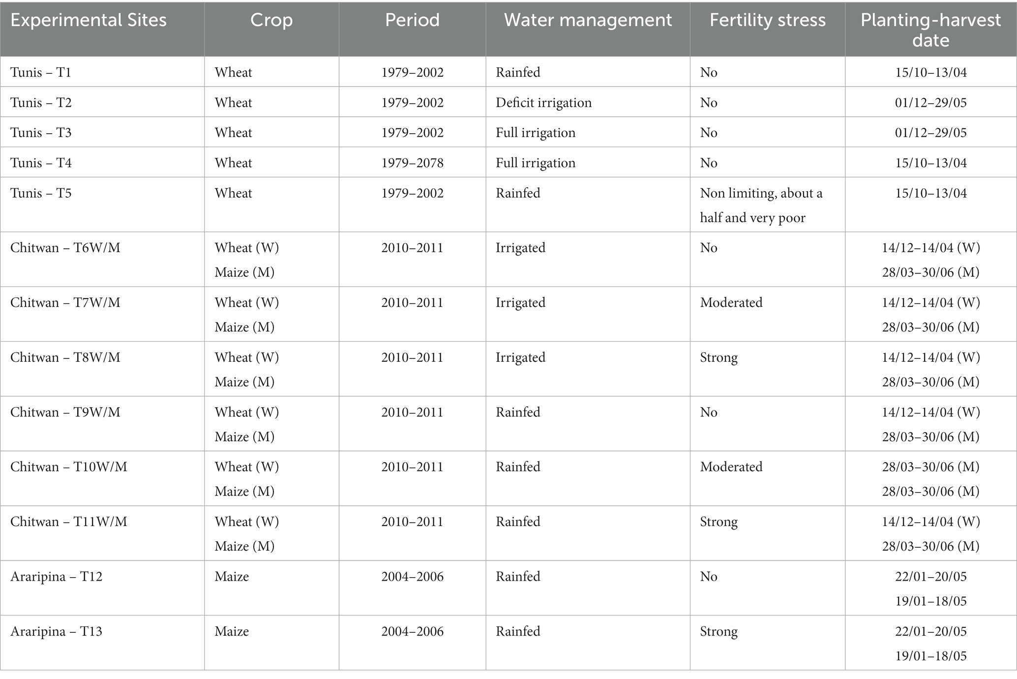
Table 1. Description of the reference experiments in Tunis and the observational experiments in Chitwan and Araripina (Source: Shrestha, 2014; van Gaelen et al., 2014; Martins et al., 2018).

For the first site, namely Tunis, Tunisia (36° 48’N, 10° 10′E), dominated by a semiarid climate, we compared simulation results of AQF and AquaCrop GUI to assess the differences in the simulation outputs between both codes. The experiments were selected from the dataset provided with the AquaCrop installation package, used for checking and training the software (Raes and van Gaelen, 2016). We compared the final yield and total irrigation for successive growing seasons generated by both versions. In addition, daily biomass, canopy cover, and water contents simulations were compared through the first growing season. The experiments include simulations under rainfed, partial, and full irrigation for different initial conditions (T1–T3, respectively); a comparison of both codes’ performance for a hundred-year simulation (T4); and models outputs for a different level of fertility stress (T5) using the fertility stress data of Table 2. The initial soil condition for experiments T1, T4, and T5 is wet topsoil and dry subsoil, wilting point for T2 and T3, and field capacity for T6 to T13.

TABLE 2

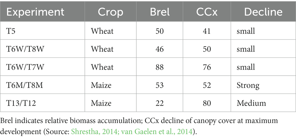
Table 2. Input data used to calibrate the fertility stress experiments.

Several experiments indicated as T6–T11 in Table 1, were carried out for wheat (W) and maize (M) in the second experimental site, Chitwan, Nepal (27°39’ N, 84°21′ E), characterized by a tropical monsoon climate with high humidity. In these experiments, we assessed AQF simulations against field observations regarding water and fertility stress on crop productivity for different stress levels (Table 2). First, we calibrated fertility stress coefficients using the two fertility stress levels in the case of wheat and a single point of the effect of fertility stress for maize (Table 2). Then, we evaluated the stress due to the combination of water and soil fertility stress for maize (M) and wheat (W) experiments (T6–T11).

The third experimental site, Araripina (7°55’ S, 40°56’ W), is located in Brazil’s semiarid region, which is characterized by highly variable interannual and intra-seasonal rainfall. Maize is produced using low technological resources. Consequently, yield gaps are the largest in the country. We used AQF with a seasonal climate forecast model to predict maize yield for two different experiments (T12 and T13). The crop forecasts were compared to in-situ data under optimum (non-stress) fertility conditions collected by the Brazilian Agriculture Research Corporation – EMBRAPA (Martins et al., 2018); and against on-farm yield with soil fertility stress (provided by the Brazilian Institute of Geography and Statistics – IBGE, 2007). In the latter case, fertility stress parameters were calibrated based on the yield gap estimated under favorable rain conditions (2006) and then directly applied to the irregular rainy crop season (2004). In Supplementary material Section S1 provides more detailed information about experiments T1–T13.

Finally, Table 3 describes the soil types and properties of the experimental sites.

TABLE 3

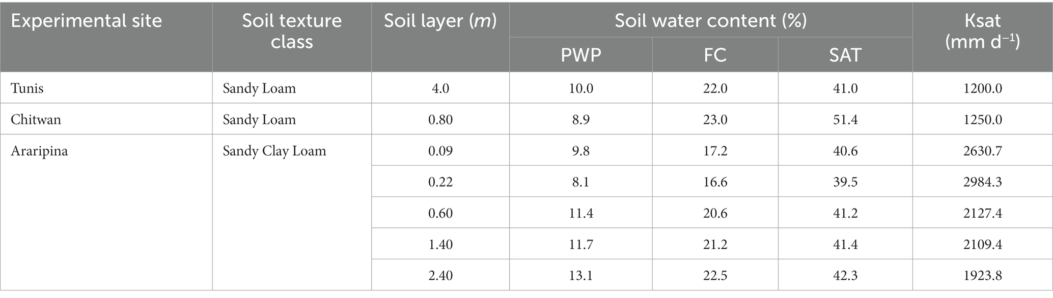
Table 3. Soil properties for the three experimental sites: PWP corresponds to the permanent wilting point; FC Field capacity; SAT water content at saturation, and Ksat saturated hydraulic conductivity (Source: Shrestha, 2014; van Gaelen et al., 2014; Martins et al., 2018).

2.3. Performances indices

We used statistical indices to compare the outputs of both versions and simulations against field observations: the coefficient of determination (r²); the index of agreement (d) (Willmott et al., 1985; Legates and McCabe Jr, 1999); the normalized root-mean-square error (RMSEn) (Loague and Green, 1991); and the mean bias error (MBE) calculated through the following equations:

$\begin{array}{ll}r2=\left(\frac{{{\displaystyle \sum }}_{\mathrm{i}=1}^{\mathrm{n}}\left(R_{\mathrm{i}}-\mathrm{M}\right)\left({\mathrm{P}}_{\mathrm{i}}-{\mathrm{M}}_{\mathrm{E}}\right)}{\sqrt{{{\displaystyle \sum }}_{\mathrm{i}=1}^{\mathrm{n}}{\left({\mathrm{R}}_{\mathrm{i}}-\mathrm{M}\right)}^2}\sqrt{{{\displaystyle \sum }}_{\mathrm{i}=1}^{\mathrm{n}}\left({\mathrm{P}}_{\mathrm{i}}-{\mathrm{M}}_{\mathrm{E}}\right)2}}\right)2& (4)\end{array}$

$\begin{array}{ll}d=1-\left[\frac{{{\displaystyle \sum }}_{i=1}^n{\left(\left|P_i-R_i\right|\right)}^2}{{{\displaystyle \sum }}_{i=1}^n{\left(\left|P_i-M\right|+\left|R_i-M\right|\right)}^2}\right]& (5)\end{array}$

$\begin{array}{ll}RMSEn=\sqrt{\frac{{{\displaystyle \sum }}_{i=1}^n{\left(P_i-R\right)}^2}{n}}\ast \frac{100}{M}& (6)\end{array}$

$\begin{array}{ll}MBE=\frac{{{\displaystyle \sum }}_{i=1}^n\left(P_i-R_i\right)}{n}& (7)\end{array}$

P_i and R_i refer to the predicted and reference values of the studied variables; n is the number of observations, M is the reference average, and ME is the predicted average. The coefficient of determination (r²) measures how well reference values are replicated by the model simulations, while the index of agreement (d) is an accuracy metric. On the other hand, the normalized RMSEn (%) calculates the relative difference between simulated versus reference data. Lastly, the mean bias error (MBE) represents the tendency of the model to overestimate (positive values) or underestimate (negative values) the reference values.

3. Results and discussion

3.1. Tunis experiments

Figure 1 compares the final yield calculated by AquaCrop GUI and AQF for the T1 experiment in Tunis. The average wheat yield simulated by AQF and AquaCrop GUI was 8.65 (±0.29) ton ha⁻¹. The mean bias error for yield was −0.004ton ha⁻¹ while the RMSEn was 0.84%. Regarding water productivity, AQF simulated 3.23 (±0.17) kg.m⁻³, while AquaCrop GUI simulated 3.20 (±0.16) kg.m⁻³.

FIGURE 1

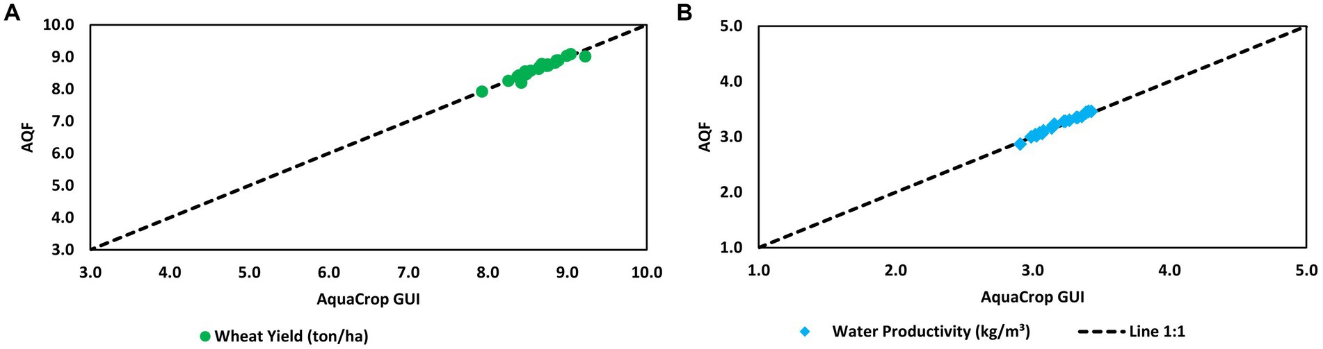
Figure 1. Comparison of AquaCrop GUI and AQF for wheat yield (A) and water productivity (B) under rainfed conditions over 1979–2002.

In supplementary material, Supplementary Figure S1 compares daily values of canopy cover development, biomass production, harvest index, and soil water content over the growing season for both models for the first year of the simulations. Although AquaCrop Fortran compared well with AquaCrop GUI simulations for all the variables tested, minor differences occurred at the end of the growing season. Daily time step comparisons revealed that AQF presented a more rapid canopy decline. In contrast, the canopy cover in the AquaCrop GUI case was less sensitive to reducing soil water content at the end of the growing season than the Fortran version. However, root water extraction and canopy cover feedback likely explain soil water content differences (Figure S1). Despite these differences, aggregated values for the whole period are very similar.

Using deficit irrigation on Tunis’s wheat for 23 years (experiment T2), AquaCrop GUI simulated an average yield of 6.22 (±1.42) ton. ha⁻¹, against 6.14 (±1.48) ton. ha⁻¹ for AquaCrop Fortran (Figure 2A). Both models produced very similar results in terms of water productivity response (Figure 2B).

FIGURE 2

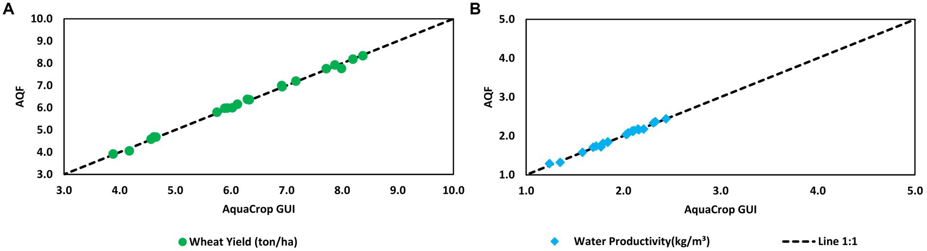
Figure 2. Comparison of AquaCrop GUI and AQF for wheat yield (A) and water productivity (B) under deficit irrigation over 1979–2002.

For the full irrigation experiment (T3), wheat yield simulated by AQF slightly overestimated AquaCrop GUI simulations (Figure 3A). Regarding the seasonal water requirements, AQF is lower than AquaCrop GUI simulations, on average 25 mm per season, equivalent to 10.7% on average (Figure 3B).

FIGURE 3

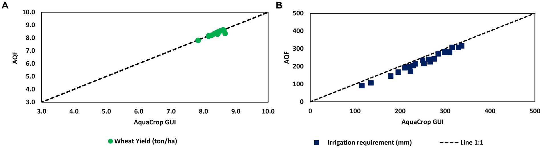
Figure 3. Comparisons of AquaCrop GUI and AQF simulations for wheat yield (A) and irrigation requirement (B) over 1979–2002.

We compared the computation time of both versions by running a long-term simulation (Experiment T4) using an i7-10510u CPU 1.80 GHz - 2.30 GHz Intel processor with 16GB RAM. While the AquaCrop GUI required approximately 215 seconds to run a hundred-year simulation (1979–2078), AQF demanded about 1 second. Results between both versions in terms of final yield, biomass and water productivity were quite similar, though AQF underestimated the AquaCrop GUI’s irrigation requirements (see Figure S2 in Supplementary material). Therefore, the efficiency of the AQF in terms of computational time opens the possibility of a whole new range of numerical experiments and detailed simulations in an operational crop forecast system. Moreover, test runs of AQF for the seasonal forecasts experiments of Martins et al. (2018) and crop productivity predictions under climate change (Martins et al., 2019, 2023) corroborated the efficiency of the code in terms of computational time and reproducibility.

Finally, in Figure 4, we compared the outputs of AQF and AquaCrop GUI for different values of the soil fertility stress. The average wheat yields simulated by AQF were 8.65 (±0.29), 4.15 (±0.15), and 2.53 (±0.10) ton ha^–1, for non-limiting, about a half, and very poor soil fertility, respectively, while the correspondent values of AquaCrop GUI were, respectively, 8.65 (±0.29), 4.46 (±0.12), and 2.34 (±0.06) ton ha^–1. Water productivity – WP was also very close in all simulations: AQF simulated an average of 3.23 (±0.17), 1.75 (±0.14), and 1.19 (±0.13) kg.m⁻³ for, respectively, non-limiting, about a half, and very poor fertility level; while AquaCrop GUI estimations were 3.20 (±0.15), 1.76 (±0.20) and 1.04 (±0.11) kg.m⁻³.

FIGURE 4

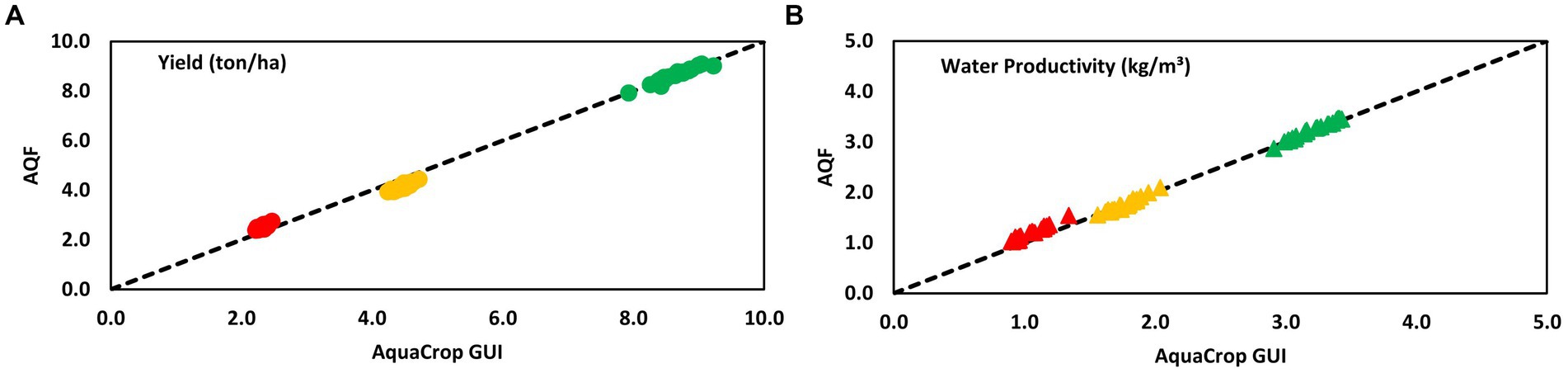
Figure 4. Comparisons of AquaCrop GUI and AQF simulations of wheat yield (ton. ha^-1) (A) and water productivity (kg.m^-3) (B) under different soil fertility conditions. Green, yellow, and red points indicate non-limiting, about a half, and very poor soil fertility, respectively.

The daily time-step analysis (Supplementary Figure S2) revealed that AQF presented a faster canopy decline, particularly in the case of very poor soil fertility, resulting in an earlier end of the crop cycle compared to the GUI version. The length of the growing season in AquaCrop GUI appeared to be insensitive to the fertility stress, and an abrupt decline in canopy cover simulations was observed at the end of the cycle. Contrary to canopy development, the growth rate of biomass and yield is higher in AQF, compensating for the effects of a shorter cycle, resulting in similar values of both versions at the end of the season. These differences are qualitatively similar to those observed in experiment T1 (Supplementary Figure S1).

The analysis results in terms of the performance indices, resulting in both models’ comparisons, are presented in Supplementary Table S1. In general, differences among both versions were minor (less than 10.5%), except for the net irrigation requirements (Supplementary Figure S2), where differences among models reached 23.6% in 100 years of simulation (T4). In this case, daily time-step results (data not shown) indicated that, during very dry periods, AquaCropGUI generated lower moisture values at the top of the soil profile compared to AQF. Since net irrigation is determined by the amount of water needed to keep the soil profile to field capacity in the root zone, a drier soil profile results in a higher irrigation requirement. Nonetheless, we verified that the net irrigation requirements in AQF were similar to those of AquaCrop-OS for the same experiment (Foster et al., 2017).

A comparison of T1–T5 revealed a close agreement between AquaCrop GUI and AQF for the same input data. Therefore, slight differences in the outputs of the Fortran and the GUI versions of AquaCrop are expected, which cannot be analyzed in detail because AquaCrop GUI is not open-source. Moreover, those differences are of the same order as those reported in the AquaCropR (Rodriguez and Ober, 2019); and AquaCrop-OSPy (Kelly and Foster, 2021).

3.2. Observational experiments in Chitwan

Table 4 shows the fertility stress shape coefficients calibrated by AQF for wheat and maize, using input data from the fertility response of Table 2.

TABLE 4

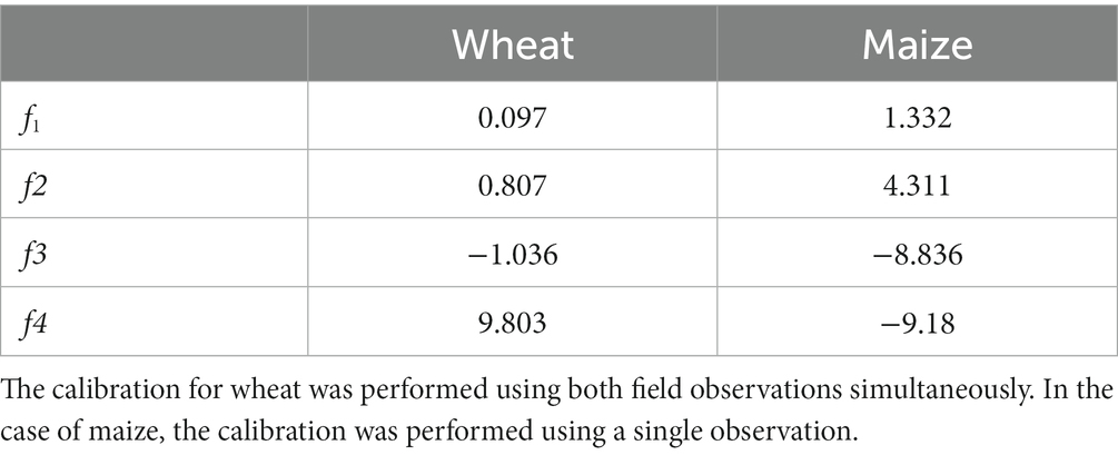
Table 4. Fertility stress shape coefficients calibrated for wheat and maize in AQF.

Figure 5 compares field observations and simulations generated using the fertility stress coefficients of Table 4 for different water and fertility stress levels, for wheat and maize, in terms of final yield and biomass.

FIGURE 5

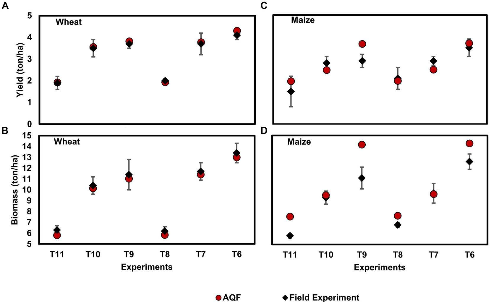
Figure 5. Comparison of final yield from wheat (A) and maize (C) and final biomass for wheat (B) and maize (D). T6: Irrigated without fertility stress; T7: Irrigated with moderate stress fertility; T8: Irrigated with strong fertility stress; T9: Rainfed without fertility stress; T10: Rainfed with moderate fertility stress and T11: Rainfed with strong fertility stress. Vertical bars represent the standard deviation.

The average error (RMSEn) in estimating wheat yield in the experiments in Figure 5A was 3.44%, while in the case of biomass, the RMSEn was 3.67% (Figure 5B). The most significant discrepancy occurred in T7W (experiment with moderate fertility stress). AQF overestimated the observation by 0.3 ton ha⁻¹.

In the case of maize, AquaCrop Fortran simulations overestimated the observed final biomass (Figure 5D) with an error (RMSEn) of 13.94% compared to experimental values. Although the absolute error in final yield, measured by the MBE, was quite smaller than the biomass error (Figure 5C).

A possible explanation for the excellent fit between AQF simulation and observation for wheat compared to maize simulations might be related to the fact that more detailed field information about fertility stress is available in the first case (Table 2).

Figure 6 compares field observations and the simulations for the entire growing cycle of AQF for wheat (left column) and maize (right column) for experiments T6, T7, and T8. Simulations of biomass, canopy cover development, and soil water content for AQF showed results close to observations throughout the entire growing cycle (Figures 6A–C).

FIGURE 6

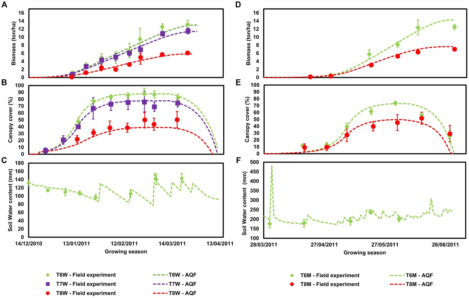
Figure 6. Biomass accumulation (A and D), canopy cover development (B and E), and soil water content (C and F). The left column shows the simulation for wheat, while the right column shows the simulation for maize. Vertical bars represent the standard deviation.

Although AQF simulations were also close to observation for maize (Figures 6D–F), they overestimated the final biomass for experiment T6M (Figure 6D). On the other hand, for strong soil fertility stress conditions (experiment T8M), AQF accurately predicted the final biomass (Figure 6D), though it generated a premature end of the canopy development cycle compared to observations (Figure 6E).

The only simulation in that AQF exceeded 20% in error was canopy cover in T8M (Figure 6E), this experiment presented strong stress fertility, and AquaCrop Fortran presented an error of 33.7%. As shown in Figure 6E, the model performance was affected by the observation of canopy cover greater than the maximum value used for calibration, recorded at the beginning of the senescence stage. It is unclear if this is caused by measurement error or late-season canopy recovery, which was unable to be captured by AQF.

For overall experiments, the final yield errors (RMSEn) of AQF varied from 3.44 to 13.9%, while biomass ranged from 3.6 to 15%, and water content was between 6.5 to 14.9%. Regarding canopy cover, errors varied from 3.9 to 33.7%, with only one simulation exceeding the error of 20% (T8M), as explained before. Table S2 (Supplementary material) presents the performance statistic for various output variables against observations in detail.

Statistical indices of all AQF simulations showed very good performance, precision close to one, and RMSEn values less than 10% in most experiments.

3.3. Aquacrop Fortran application to an operational crop forecast system

To demonstrate the value of AQF in an operational crop forecast system, Figure 7 presents an example of a forecast 45 days before the harvest for a case study in Araripina for two different crop seasons and both optimum and limited soil fertility conditions.

FIGURE 7

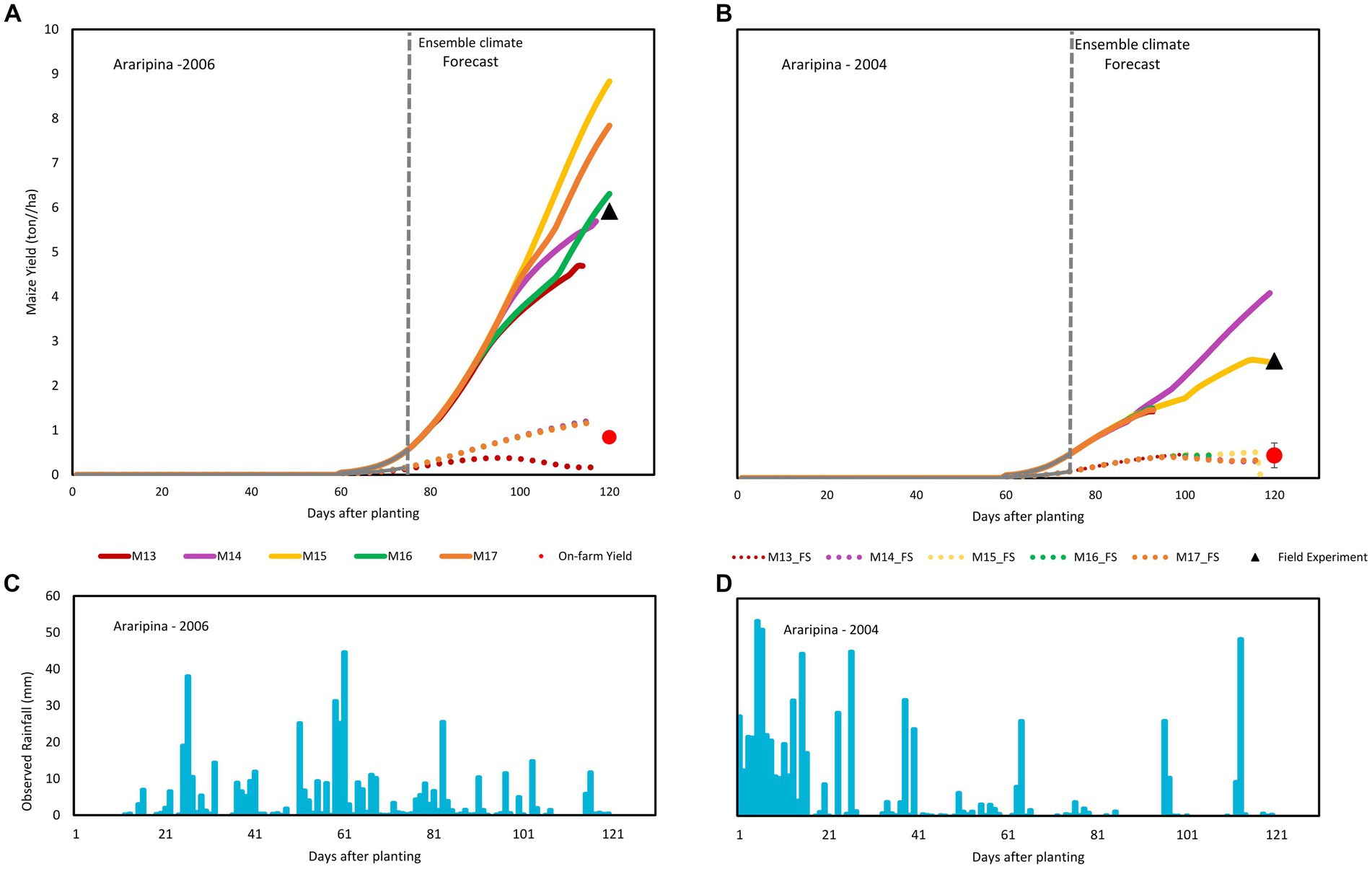
Figure 7. Ensemble Crop forecast Simulation for Araripina (Brazil) for 2006 (A) and 2004 (B) using five members from Eta regional climate model denoted as M13–M17. The continuous lines represent the simulations without soil fertility stress, while the dotted lines represent the fertility stress simulation. The black triangle represents the final maize yield of the controlled field experiment (OBS), while the red diamond indicates the average on-farm yield. (C,D) show the observed rainfall recorded during both seasons.

Figure 7A indicates considerable spread among members of the forecast for the wet year, particularly for non-fertility stress conditions (experiment T12, continuous lines) and to a lesser degree for on-farm yield under stressed fertility conditions (experiment T13, dotted lines), indicating that under optimum soil fertility, the forecast is more sensitive to rainfall variability among the members. The average maize yield forecasted by the five members is 6.7 ton ha⁻¹, compared to 5.9 ton ha⁻¹ of the controlled field experiment, significantly greater than the average 1.5 ton ha⁻¹ on-farm yield predicted by the forecast members and the 0.9 ton ha⁻¹ on-farm yield of the official statistics.

Assessments for the 2004 dry year (Figure 7B) show a much lower spread among members for both controlled (T12) and soil fertility stress (T13) experiments, which is expected since rainfall throughout the crop season was scarce. The average productivity of the member’s ensemble was forecasted at 2.25 ton ha⁻¹, a value near 2.6 ton ha⁻¹ of the controlled field experiment. On-farm yield for soil fertility stress simulations was estimated at 0.5 ton ha⁻¹, close to 0.4 ton ha⁻¹ from the value recorded by the official statistics.

An application of AQF for estimating on-farm yield in the semiarid Northeast of Brazil demonstrated the versatility of the software for application in operational forecast systems, particularly in vulnerable regions that depend on subsistence agriculture, where the accounting of the soil fertility level is essential to reach the correct forecast.

4. Conclusion

We presented an open-source version of a crop model based on AquaCrop aimed for operational application in crop forecast systems with high computational costs, including the effect of soil fertility stress on productivity.

The main advantage of a high-level code like AQF is the flexibility to modify inputs and outputs files and couple it with other models, like climate and hydrological models. Besides, coefficient calculations and estimations can be modified to suit specific user purposes. However, it creates several risks because unintended changes in the code might result in incorrect results and jeopardize the model version’s reliability. Therefore, any further changes in the source code should be done with caution, with expert knowledge in Fortran coding and capable of understanding the physical processes involved in the soil–plant-atmosphere relationship.

Finally, the software presented in this study does not intend to compete with or reduce the usefulness of the AquaCrop GUI. On the contrary, it offers an alternative more suitable for a science community’s applications and crop monitoring close to our work and needs, such as the operational crop forecast systems we are developing for the Northeast of Brazil, which is feasible to implement in other regions of the world. Given that climate change scenarios predict the intensification of climate extremes in several regions of the world, future crop productivity will be affected. To examine adaptation strategies to minimize the negative effects of climate change, tools capable to produce a timely early warning and long-term simulations over large areas, such as AQF, will be needed.

Data availability statement

The original contributions presented in the study are included in the article/Supplementary material, further inquiries can be directed to the corresponding author.

Author contributions

JT code development, data analysis, and manuscript review. MM simulation tests, data analysis, and writing the original draft. NS provided experimental data and final review. All authors contributed to the article and approved the submitted version.

Funding

The authors would like to thank the São Paulo Research Foundation – FAPESP, under Grant Numbers 2022/00917-0 and 2017/22269-2, and the National Council for Research and Development - CNPq, under Grant Agreements 304695/2020–3 and 428995/2018–7 for their support in the development of this study.

Conflict of interest

The authors declare that the research was conducted in the absence of any commercial or financial relationships that could be construed as a potential conflict of interest.

Publisher’s note

All claims expressed in this article are solely those of the authors and do not necessarily represent those of their affiliated organizations, or those of the publisher, the editors and the reviewers. Any product that may be evaluated in this article, or claim that may be made by its manufacturer, is not guaranteed or endorsed by the publisher.

Supplementary material

The Supplementary material for this article can be found online at: https://www.frontiersin.org/articles/10.3389/fsufs.2023.1084728/full#supplementary-material

Footnotes

1. ^Available at http://www.fao.org/aquacrop/en/.

References

Abrha, B., Delbecque, N., Raes, D., Tsegay, A., Todorovic, M., Heng, L., et al. (2012). Sowing strategies for barley (hordeum vulgare l.) based on modelled yield response to water with AquaCrop. Exp. Agric. 48, 252–271. doi: 10.1017/S0014479711001190

CrossRef Full Text | Google Scholar

Akumaga, U., Tarhule, A., and Yusuf, A. A. (2017). Validation and testing of the FAO AquaCrop model under different levels of nitrogen fertilizer on rainfed maize in Nigeria, West Africa. Agric. For. Meteorol. 232, 225–234. doi: 10.1016/j.agrformet.2016.08.011

CrossRef Full Text | Google Scholar

Becker-Reshef, I., Barker, B., Humber, M., Puricelli, E., Sanchez, A., Sahajpal, R., et al. (2019). The GEOGLAM crop monitor for AMIS: assessing crop conditions in the context of global markets. Glob. Food Sec. 23, 173–181. doi: 10.1016/j.gfs.2019.04.010

CrossRef Full Text | Google Scholar

Bento, V. A., Russo, A., Dutra, E., Ribeiro, A. F., Gouveia, C. M., and Trigo, R. M. (2022). Persistence versus dynamical seasonal forecasts of cereal crop yields. Sci. Rep. 12, 7422–7411. doi: 10.1038/s41598-022-11228-2

PubMed Abstract | CrossRef Full Text | Google Scholar

Bussay, A., van der Velde, M., Fumagalli, D., and Seguini, L. (2015). Improving operational maize yield forecasting in Hungary. Agric. Syst. 141, 94–106. doi: 10.1016/j.agsy.2015.10.001

CrossRef Full Text | Google Scholar

Chibarabada, T. P., Modi, A. T., and Mabhaudhi, T. (2020). Calibration and evaluation of AquaCrop for groundnut (Arachis hypogaea) under water deficit conditions. Agric. For. Meteorol. 281:107850. doi: 10.1016/j.agrformet.2019.107850

CrossRef Full Text | Google Scholar

Chitsiko, R. J., Mutanga, O., Dube, T., and Kutywayo, D. (2022). Review of current models and approaches used for maize crop yield forecasting in sub-Saharan Africa and their potential use in early warning systems. Phys. Chem. Earth 127:103199. doi: 10.1016/j.pce.2022.103199

CrossRef Full Text | Google Scholar

Christian, J. I., Basara, J. B., Hunt, E. D., Otkin, J. A., Furtado, J. C., Mishra, V., et al. (2021). Global distribution, trends, and drivers of flash drought occurrence. Nat. Commun. 12:6330. doi: 10.1038/s41467-021-26692-z

PubMed Abstract | CrossRef Full Text | Google Scholar

de Roos, S., de Lannoy, G., and Raes, D. (2020). From the field-scale Aquacrop model to a regional gridded crop model: initial evaluation over Europe, EGU general assembly 2020, online, 4–8 May 2020, EGU2020-5290. doi: 10.5194/egusphere-egu2020-5290

CrossRef Full Text | Google Scholar

de Wit, A., Boogaard, H., Fumagalli, D., Janssen, S., Knapen, R., van Kraalingen, D., et al. (2018). 25 years of the WOFOST cropping systems model. Agric. Syst. 168, 154–167. doi: 10.1016/j.agsy.2018.06.018

CrossRef Full Text | Google Scholar

Dhakar, R., Sehgal, V. K., Chakraborty, D., Sahoo, R. N., Mukherjee, J., Ines, A. V., et al. (2022). Field scale spatial wheat yield forecasting system under limited field data availability by integrating crop simulation model with weather forecast and satellite remote sensing. Agric. Syst. 195:103299. doi: 10.1016/j.agsy.2021.103299

CrossRef Full Text | Google Scholar

Fischer, R. A. (2015). Definitions and determination of crop yield, yield gaps, and of rates of change. Field Crop Res. 182, 9–18. doi: 10.1016/j.fcr.2014.12.006

CrossRef Full Text | Google Scholar

Foster, T. N., Brozović, N., Butler, A. P., Neale, C. M. U., Raes, D., Steduto, P., et al. (2017). AquaCrop-OS: an open source version of FAO's crop water productivity model. Agric. Water Manag. 181, 18–22. doi: 10.1016/j.agwat.2016.11.015

CrossRef Full Text | Google Scholar

García-Vila, R., and Fereres, E. (2012). Combining the simulation crop model AquaCrop with an economic model for the optimization of irrigation management at farm level. Eur. J. Agron. 36, 21–31. doi: 10.1016/j.eja.2011.08.003

CrossRef Full Text | Google Scholar

Geerts, S., and Raes, D. (2009). Deficit irrigation as an on-farm strategy to maximize crop water productivity in dry areas. Agric. Water Manag. 96, 1275–1284. doi: 10.1016/j.agwat.2009.04.009

CrossRef Full Text | Google Scholar

Guo, D., Zhao, R., Xing, X., and Ma, X. (2019). Global sensitivity and uncertainty analysis of the AquaCrop model for maize under different irrigation and fertilizer management conditions. Arch. Agron. Soil Sci. 66, 1115–1133. doi: 10.1080/03650340.2019.1657845

CrossRef Full Text | Google Scholar

Holzworth, D., Huth, N. I., Fainges, J., Brown, H., Zurcher, E., Cichota, R., et al. (2018). APSIM next generation: overcoming challenges in modernising a farming systems model. Environ. Model Softw. 103, 43–51. doi: 10.1016/j.envsoft.2018.02.002

CrossRef Full Text | Google Scholar

Hoogenboom, G., Porter, C. H., Boote, K. J., Shelia, V., Wilkens, P. W., Singh, U., et al. (2019). “The DSSAT crop modeling ecosystem” in Advances in crop modeling for a sustainable agriculture. ed. K. J. Boote (Cambridge, United Kingdom: Burleigh Dodds Science Publishing), 173–216. http://dx.doi.org/10.19103/AS.2019.0061.10

Google Scholar

IBGE. (2007). Produção Agrícola Municipal. Disponível em. Available at: https://sidra.ibge.gov.br/tabela/839#notas-tabela ().

Google Scholar

Kelly, T. D., and Foster, T. (2021). AquaCrop-OSPy: bridging the gap between research and practice in crop-water modeling. Agric. Water Manag. 254:106976. doi: 10.1016/j.agwat.2021.106976

CrossRef Full Text | Google Scholar

Legates, D. R., and McCabe, G. J. Jr. (1999). Evaluating the use of "goodness-of-fit" measures in hydrologic and hydroclimatic model validation. Water Resour. Res. 35, 233–241. doi: 10.1029/1998WR900018

CrossRef Full Text | Google Scholar

Loague, K., and Green, R. E. (1991). Statistical and graphical methods for evaluating solute transport models: overview and application. J. Contam. Hydrol. 7, 51–73. doi: 10.1016/0169-7722(91)90038-3

CrossRef Full Text | Google Scholar

Martins, M. A., Tomasella, J., Bassanelli, H. R., Paiva, A. C. E., Vieira, R. M. S., Canamary, E. A., et al. (2023). On the sustainability of paddy rice cultivation in the Paraíba do Sul river basin (Brazil) under a changing climate. J. Clean. Prod. 386:135760. doi: 10.1016/j.jclepro.2022.135760

CrossRef Full Text | Google Scholar

Martins, M. A., Tomasella, J., and Dias, C. G. (2019). Maize yield under a changing climate in the Brazilian northeast: impacts and adaptation. Agric. Water Manag. 216, 339–350. doi: 10.1016/j.agwat.2019.02.011

CrossRef Full Text | Google Scholar

Martins, M. A., Tomasella, J., Rodriguez, D. A., Alvalá, R. C. S., Giarolla, A., Garofolo, L. L., et al. (2018). Improving drought management in the Brazilian semiarid through crop forecasting. Agric. Syst. 160, 21–30. doi: 10.1016/j.agsy.2017.11.002

CrossRef Full Text | Google Scholar

MCYFS. MARSWiki, (2022). Available at: http://marswiki.jrc.ec.europa.eu/agri4castwiki/index.php/Main_Page (Accessed June 21, 2022).

Google Scholar

Ministerial Declaration (2011). “Action plan on food price volatility and agriculture” in Meeting of G20 agriculture ministers Paris, 22 and 23 June 2011. Available at: https://reliefweb.int/report/world/ministerial-declaration-action-plan-food-price-volatility-and-agriculture-meeting-g20 (Accessed June 14, 2023).

Google Scholar

Muluneh, A., Stroosnijder, L., Keesstra, S., and Biazin, B. (2016). Adapting to climate change for food security in the Rift Valley dry lands of Ethiopia: supplemental irrigation, plant density and sowing date. J. Agric. Sci. 155, 703–724. doi: 10.1017/S0021859616000897

CrossRef Full Text | Google Scholar

Otkin, J., Svoboda, M., Hunt, E., Ford, T., Anderson, M., Hain, C., et al. (2017). Flash droughts: a review and assessment of the challenges imposed by rapid-onset droughts in the United States. Bull. Am. Meteorol. Soc. 99, 911–919. doi: 10.1175/BAMS-D-17-0149.1

CrossRef Full Text | Google Scholar

Pirmoradian, N., and Davatgar, N. (2019). Simulating the effects of climatic fluctuations on rice irrigation water requirement using AquaCrop. Agric. Water Manag. 213, 97–106. doi: 10.1016/j.agwat.2018.10.003

CrossRef Full Text | Google Scholar

Raes, D., Steduto, P., Hsiao, T. C., and Fereres, E. (2009). AquaCrop-the FAO crop model to simulate yield response to water: II. Main algorithms and software description. Agron. J. 101, 438–447. doi: 10.2134/agronj2008.0140s

CrossRef Full Text | Google Scholar

Raes, D., Steduto, P., Hsiao, T. C., and Fereres, E.. (2018). AquaCrop reference manual, AquaCrop version 4.0. Rome, Italy: FAO.

Google Scholar

Ranjbar, A., Rahimikhoob, A., Ebrahimian, H., and Varavipour, M. (2019). Assessment of the AquaCrop model for simulating maize response to different nitrogen stresses under semi-arid climate. Commun. Soil Sci. Plant Anal. 50, 2899–2912. doi: 10.1080/00103624.2019.1689254

CrossRef Full Text | Google Scholar

Rodriguez, A. V. C., and Ober, E. S. (2019). AquaCropR: crop growth model for R. Agronomy 9:378. doi: 10.3390/agronomy9070378

CrossRef Full Text | Google Scholar

Sandhu, R., and Irmak, S. (2019). Performance of AquaCrop model in simulating maize growth, yield, and evapotranspiration under rainfed, limited and full irrigation. Agric. Water Manag. 223:105687. doi: 10.1016/j.agwat.2019.105687

CrossRef Full Text | Google Scholar

Shrestha, N. (2014). Improving cereal production in the Terai region of Nepal. Assessment of field management strategies through a model based approach. Dissertation thesis. KU Leuven.

Google Scholar

Sietz, D., Untied, B., Walkenhorst, O., Lüdeke, M. K. B., Mertins, G., Petschel-Held, G., et al. (2006). Smallholder agriculture in Northeast Brazil: assessing heterogeneous human-environmental dynamics. Reg. Environ. Chang. 6, 132–146. doi: 10.1007/s10113-005-0010-9

CrossRef Full Text | Google Scholar

Steduto, P., Hsiao, T. C., Raes, D., and Fereres, E. (2009). AquaCrop—the FAO crop model to simulate yield response to water: I concepts and underlying principles. Agron. J. 101, 426–437. doi: 10.2134/agronj2008.0139s

CrossRef Full Text | Google Scholar

Van der Velde, M., and Nisini, L. (2018). Performance of the MARS-crop yield forecasting system for the European Union: assessing accuracy, in-season, and year-to-year improvements from 1993 to 2015. Agric. Syst. 168, 203–212. doi: 10.1016/j.agsy.2018.06.009

PubMed Abstract | CrossRef Full Text | Google Scholar

van Gaelen, H., Tsegay, A., Delbecque, N., Shrestha, N., Garcia, M., Fajardo, H., et al. (2014). Asemi-quantitative approach for modelling crop response to soil fertility:evaluation of the AquaCcrop procedure. J. Agric. Sci. 153, 1218–1233. doi: 10.1017/S0021859614000872

CrossRef Full Text | Google Scholar

van Oort, P. A. J., and Zwart, S. J. (2017). Impacts of climate change on rice production in Africa and causes of simulated yield changes. Glob. Change Biol. 24, 1029–1045. doi: 10.1111/gcb.13967.00

CrossRef Full Text | Google Scholar

Raes, D., and Van Gaelen, H. (2016). AquaCrop training handbooks—Book II running AquaCrop; Food and Agriculture Organization of the United Nations: Rome, Italy.

Google Scholar

Vieira, R. M. S. P., Sestini, M. F., Tomasella, J., Marchezini, V., Pereira, G. R., Barbosa, A. A., et al. (2020). Characterizing spatio-temporal patterns of social vulnerability to droughts, degradation and desertification in the Brazilian northeast. Environ. Sustain. Indic. 5:100016. doi: 10.1016/j.indic.2019.100016

CrossRef Full Text | Google Scholar

Vijay, S., and Srinivas, V. V. (2022, 2022). Meteorological flash droughts risk projections based on CMIP6 climate change scenarios. NPJ Clim. Atmos. Sci. 5:77. doi: 10.1038/s41612-022-00302-1

CrossRef Full Text | Google Scholar

Willmott, C. J., Ackleson, S. G., Davis, R. E., Feddema, J. J., Klink, K. M., Legates, D. R., et al. (1985). Statistics for the evaluation and comparison of models. J. Geophys. Res. 90, 8995–9005. doi: 10.1029/JC090iC05p08995

CrossRef Full Text | Google Scholar