Effects of biochar and ligneous soil amendments on greenhouse gas exchange during extremely dry growing season in a Finnish cropland

Organic soil amendments such as manure, biochar and compost are among the most efficient and widely used methods to increase soil carbon sequestration in agricultural soils. Even though their benefits are well known, many wood-derived materials are not yet utilized in Nordic agriculture due to a lack of incentives and knowledge of their effects in the local climate. We studied greenhouse gas exchange, plant growth and soil properties of a clay soil cultivated with oat in southern Finland in an extremely dry year. Two years earlier, the field was treated with three ligneous soil amendments—lime-stabilized fiber from the pulp industry, willow biochar and spruce biochar—which we compared against fertilized and non-fertilized controls. We found that the soil amendments increased porosity and the mean soil water holding capacity, which was most noticeable in plots amended with spruce biochar. There was a trend indicating that the mean yield and overall biomass production were larger in plots with soil amendments; however, the difference to unamended control was seldom significant due to the high variance among replicates. Manual chamber measurements revealed that carbon dioxide and methane exchange rates were reduced most probably by the exceptionally hot and dry weather conditions, but no differences could be found between the amended and unamended treatments. The nitrous oxide emissions were significantly smaller from the vegetated soil amended with willow biochar compared with the unamended control. Emissions from non-vegetated soil, representing heterotrophic respiration, were similar but without significant differences between treatments. Overall, the studied soil amendments indicated positive climatic impact two years after their application, but further research is needed to conclusively characterize the specific effects of organic soil amendments on processes affecting greenhouse gas exchange and plant growth.

Introduction

The targets of the Paris Agreement cannot be reached without effective ways to remove carbon dioxide (CO₂) from the atmosphere (Millar et al., 2017; Minasny et al., 2017). Therefore, intensification of land CO₂ sinks has been suggested as a solution, for example, by managing agricultural soils, increasing afforestation, or restoring degraded soils and ecosystems (Griscom et al., 2017; Roe et al., 2019). Climate-smart management in agriculture often advocates the use of carbon-rich materials as soil amendments or fertilizers to sequester carbon (C) into long lasting forms. This has the potential to mitigate climate change and to support soil fertility (Rosenstock et al., 2016) by increasing soil organic carbon (SOC) content, which promotes soil structure, soil water retention (Rawls et al., 2003; Bronick and Lal, 2005), as well as supporting nutrient cycling and microbial activity (Biederman and Harpole, 2013; Wang et al., 2016).

Biochar is currently considered the most promising option for long-term C sequestration (Lehmann et al., 2006; Woolf et al., 2010; Griscom et al., 2017; Bai et al., 2019; Smith et al., 2020) due to its resistance to decomposition (Wang et al., 2016). However, its effectiveness may be limited in areas of high natural SOC content because of possible C saturation or short-term priming effects, even though the long-term positive effects are often considered to outweigh the negative (Smith, 2005; Zimmerman et al., 2011; Wang et al., 2016). In addition, many of the additional benefits to soil fertility have been observed mainly with coarse textured and highly weathered tropical soils (Jeffery et al., 2017). Moreover, agricultural practices that provide C sequestration may have other climatic impacts, which can be either adverse or beneficial. For example, soil amendments are likely to change soil hydrological and thermal properties (Gupta et al., 1977; Abu-Hamdeh and Reeder, 2000; Rawls et al., 2003; Usowicz et al., 2016), while introducing external inputs of organic C into the soil system that may thereby reinforce unwanted microbial activity, possibly enhancing the production of nitrous oxide (N₂O) or methane (CH₄). To ensure that the overall effect of these management practices is favorable also in fine textured boreal soils, it is important to quantify the net climatic effect of different soil amendments in local conditions.

Most mineral soils cultivated in southern Finland are lacustrine sediments consisting of fine-textured deposits (Mokma et al., 2000; Ylihalla and Mokma, 2001; Matschullat et al., 2018) with organic matter content of 3–12% (Lemola et al., 2018). These clay soils are often reliant on intensive soil management and annual soil frost to loosen the soil. Moreover, the annual precipitation mostly exceeds the annual evapotranspiration, which together with naturally high water tables make these cultivated soils dependent on artificial drainage to prevent waterlogging. As a result, the intensive soil management has greatly influenced the soil formation of these young agricultural soils (Yli-Halla et al., 2009), and together with a warming climate, it has contributed to the current decline of SOC observed throughout Finland (Heikkinen et al., 2013). Consequently, implementing organic amendments into the cultivation regime may provide an opportunity to improve soil structure and to convert agricultural soils from current sources of C to sinks (Paustian et al., 2016; Bai et al., 2019; Smith et al., 2020).

In Finland, wood derived side streams i.e., ligneous biomasses are produced in large quantities. For example, pulp and paper industry produces almost as much biomass as wastewater treatment (Tampio et al., 2018) making it promising future source for soil amendments in Finland. Several studies have reported that pulp residuals increase soil C content and subsequently soil water holding capacity, one year after their application (Foley and Cooperband, 2002; Chow et al., 2003). However, Beyer et al. (1997) reported that the effects of pulp sludge on soil organic matter content disappeared after one year. Zibilske et al. (2000) and Price and Voroney (2007) suggested that the positive effects could be maintained through repeated applications. On the other hand, Rasa et al. (2021) found that a single application of pulp sludge had only minor effect on soil C content, but reduced soil erodability, even after four years. The inconsistencies concerning the persistence of pulp derived C and the longevity of its effects on soil properties call for further studies.

Our aim was to assess the climatic impact of ligneous soil amendments produced from economically significant biomasses that have the potential for wider application in Finnish agricultural soils. We had three specific research questions:

• Do the soil amendments affect soil physico-chemical properties in a way that would benefit soil fertility?

• Do the soil amendments affect net primary production (NPP), i.e., growth of biomass?

• Do the soil amendments affect greenhouse gas (GHG) exchange between agricultural soil and atmosphere?

For this purpose, we measured soil properties, biomass growth and the GHG exchange of a clay soil growing oat in southern Finland two years after the application of three different soil amendments and compared the effects of the amendments with fertilized and non-fertilized controls. We also monitored soil and weather conditions, which turned out to be important factors affecting plant growth and soil activity during the measuring campaign.

Materials and methods

Site and weather station

The study took place in 2018 at Qvidja farm (60° 17′ 44″ N 22° 23′ 35″ E), located in south-western Finland in the larger geographical area called Varsinais-Suomi. The field site was chosen for its rather flat terrain with homogeneous management history and soil properties. The soil texture was classified as clay, with 54% clay, 34% silt, and 12% sand. The World Reference Base classification was Vertic Endogleyic Stagnic Cambisol (clayic). The field site has a long cultivation history, possibly dating back centuries. During recent years, it has been cultivated for wheat (five years), caraway (three years), sugar beet with oilseed rape (two years), and grass (five years). Because of the general homogeneity and young age of cultivated soils in southern Finland (Yli-Halla et al., 2009), the site may be considered representative of a typical cropland for the geographical area.

The mean annual temperature and precipitation, measured at a nearby weather station (Yltöinen, 13 km from Qvidja), equalled 5.4°C and 679 mm, respectively, between 1981 and 2010 (Pirinen et al., 2012). In 2018, the annual mean temperature and precipitation were 6.6°C and 486 mm, respectively. In 2018, there was a shortfall of precipitation in June and July compared with the long-term mean, while temperatures much higher than average were observed especially in May and July (Figure 1).

FIGURE 1

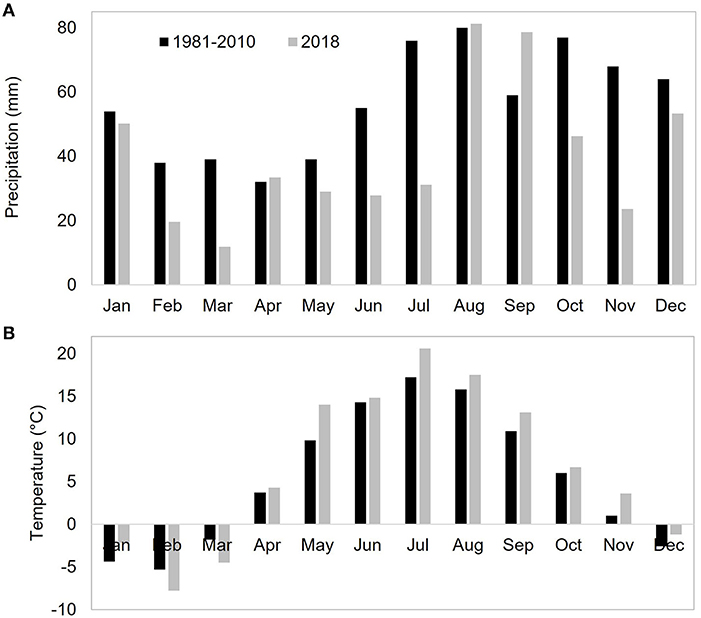
Figure 1. Monthly average precipitation (A) and temperature (B) recorded at a nearby weather station, Yltöinen, in 1980–2010 (black bars, Pirinen et al., 2012) and in 2018 (gray bars).

The weather station at the field site was established on 8 May 2018. Air temperature and humidity were measured with a Humicap HMP155 (Vaisala, Vantaa, Finland). Soil moisture was measured with an ML3 ThetaProbe sensor (Delta-T Devices, Cambridge, UK). The soil temperature was recorded from depths of 0.05, 0.10, and 0.30 m by an IKES Pt100 (Nokeval, Nokia, Finland). Photosynthetically active radiation (PAR) was measured with a PQS PAR sensor (Kipp and Zonen, Delft, the Netherlands). Precipitation was recorded with an OTT Pluvio2 (OTT HydroMet, Kempten, Germany). All measurements were logged by a Vaisala QML201C data collection board (Vaisala, Vantaa, Finland) and averaged to a 30-min resolution.

Experimental set-up and management

The experiment was launched in autumn 2016 with three replicate blocks (Figure 2) each of size 135 m × 20 m. Each of the blocks contained one randomly chosen plot (9 m × 20 m) for each of the treatments (i.e., N = 3).

FIGURE 2

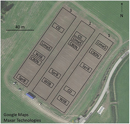
Figure 2. Experimental set-up with three replicate blocks (1–3) each having five plots, one for each treatment: C0, non-fertilized control; C80N, fertilized control; LimeS, lime-stabilized pulp sludge; SprB, spruce biochar; WilB, willow biochar.

This study included five treatments (Figure 2; Table 1): (1) C0 was a control without any soil amendment or fertilization. (2) C80N was a control without any soil amendment, but with yearly NPK fertilization. (3) LimeS (lime-stabilized pulp sludge) was amended with lime-stabilized ligneous (i.e., wood-derived) fiber sludge with yearly NPK fertilization. The fiber was applied as semi-dry mass and is a commercial product of the Soil Food Oy. For a more comprehensive description of the material, see Rasa et al. (2021). (4) SprB (spruce biochar) was amended with biochar produced through pyrolysis at 450°C from spruce (Picea abies) chips with yearly NPK fertilization. (5) WilB (willow biochar) was amended with biochar produced through pyrolysis at 450°C from willow (Salix spp.) chips with yearly NPK fertilization. Although, all the soil amendments were produced from ligneous feedstock, they each had distinct physical characteristics in semi-dry form, which made their equal use on dry weight basis difficult. Therefore, the application rates used in this study (Table 1) varied to maintain regulations concerning organic fertilizers and to agree with the rates recommended by the producers of the amendments.

TABLE 1

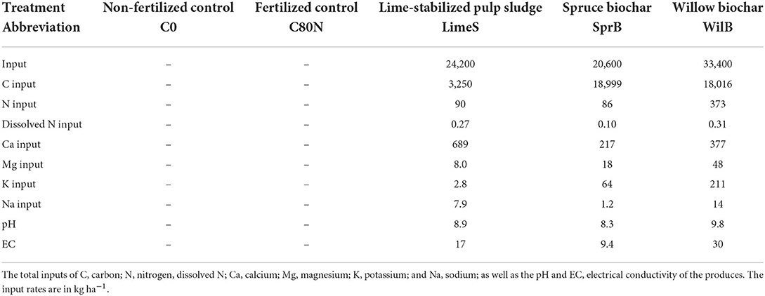
Table 1. Experimental treatments including their application rates in 2016.

After spreading the soil amendments manually in 2016, all plots were tilled with a cultivator (Horsch Terrano 3.5 FX) down to 0.10 m. In the following years, the soil management was kept within the top 0.10 m to contain the effect of the soil amendments within a limited soil layer.

In spring 2017, the field was sown with wheat and all plots except C0 were fertilized using NPK fertilizer (Yara Mila 3, 23-3-8) with 80 kg N ha⁻¹. All other practices were equal among the plots in 2017. In May 2018, the field was first prepared down to 0.05 m, and on 15 May it was sown with oat (variety Matty) using a seeder (Överum Tive CD1830), resulting in, on average, 437 germinated seeds m⁻². At the same time, all plots except for C0 were fertilized using NPK fertilizer (Yara Mila 3, 23-3-8) with 80 kg N ha⁻¹. Weeds were manually removed on 13 June. Due to extremely dry weather (Figure 1), the field was irrigated with ~40–50 mm of water during a period of 18 h on 30 June by using 11 rotary sprinklers per replicate block. Crop samples were collected with a 1.5 m wide field plot harvester (Wintersteiger, Ried, Austria) from each plot on 22 August after which the whole field was harvested and straws collected.

Soil moisture and temperature measurements

The soil temperature was measured using HOBO Pendant Temperature Loggers (UA-001-64, Onset, Bourne, MA, USA), which were installed in each plot at a depth of 0.05 m. The soil surface moisture was measured weekly from ~0.05 m with a ML3 ThetaProbe (Delta-T Devices) by manually inserting the probe into six different locations in each plot. We used the average of these measurements in the further analysis. The daily soil moisture, M, was linearly interpolated.

Soil properties

The soil water holding properties were determined from 90 undisturbed soil cores (d = 73 mm, h = 48 mm, V = 0.20 L). Six soil cores were taken from each of the 15 sampled plots: three from the soil surface (0–0.05 m) and three below the managed soil layer (0.20–0.25 m). After sampling, the cores were sealed and transported to the University of Helsinki soil science laboratory, where they were stored at 4°C before determining their soil water retention curves (SWRCs) starting in January 2019.

Each SWRC was plotted using measurements of gravimetric water content (m/m) at 0, −0.3, −6.0, −250 and −1500 kPa (Dane and Hopmans, 2002). The pressure range from 0 to −6.0 kPa was determined using the kaolin sandbox method (Eijkelkamp Agrisearch Equipment, the Netherlands) and thereafter to −1500 kPa using pressure plate extractors (Soilmoisture Equipment Corp., Santa Barbara, CA, USA) connected to a compressor (Kaeser Kompressoren, Coburg, Germany) via a pressure manifold (Soilmoisture Equipment Corp.). Plant available water (PAW) was defined as the water holding capacity at a pressure range of between −6.0 and −1500 kPa. Finally, the samples were dried at 105°C to determine their dry bulk density (ρ_bd).

Total soil C (C_tot) was determined from soil samples gathered alongside with the soil cores. The soil was first air-dried and then crushed with pestle and mortar before being analyzed with varioMAX CN analyser (Elementar Company, Langenselbold, Germany) using four analytical replicates (N = 4). Because the soil was assumed to contain negligible amount of carbonates, total soil C was assumed to equal SOC content (i.e., C_tot = SOC).

The effects of organic soil amendments on soil structure were determined by comparing them to the unamended control. Additionally, effect of spatial heterogeneity was considered by comparing the amended soil layer to the underlying unamended soil layer as well as comparing the three replicate blocks against each other using a two-way analysis of variance (ANOVA) with IBM SPSS Statistics 25.

Vegetation growth

In 2018, plant height was measured in each plot weekly from five individual oat plants using a ruler. Above- and below-ground biomass was estimated using a systematic inventory on 1 August 2018. A total of three above-ground samples and five below-ground root samples were collected per plot. The above-ground biomass was cut (ø = 0.20, m = 0.0314 m²) at a height of 0.02 m, whereas underground root samples were taken with a soil auger (ø = 0.05 m) down to 0.20 m. Three of the five root samples were taken on top of the plant rows and two in the middle of the rows. The above-ground biomass was frozen (−18°C) for 2–3 months before separating it into oat seeds, oat above-ground biomass (stems and leaves), and other biomass (weeds). Samples were then dried for 48 h at 60°C and weighed to determine their dry mass. The root samples were stored in a fridge (+6°C) for 3–7 days before soaking them in water for approximately 30 min and then manually separating the roots from bulk soil. The root biomass was then dried for 48 h at 60°C and weighed before determining loss on ignition (2 h at 550°C). During the sampling, the seeds were still developing, whereas other biomass compartments had reached maturity. Thus, we ignored the seed biomass at this stage and used biomass yield at the time of the harvest in the further analyses. The accumulation of plant biomass measured from treatments C0, C80, SprB, and WilB was described by Kalu et al. (2022). In this article, the data is reanalyzed from the perspective of carbon balance and greenhouse gas exchange. Moreover, the data was expanded to include application of LimeS as one of the treatments.

We compared the different biomass factors as well as the final height of the oat plants using a two-way ANOVA with the treatment and the replicate block as factors in R (version 3.6.1, R Core Team, 2019). We used the Shapiro–Wilk test prior to the analysis for testing normality (p > 0.05).

Greenhouse gas flux measurements

Component fluxes

We used three variations of the darkened chamber technique to measure CO₂, N₂O, and CH₄ exchange: (1) the whole ecosystem flux (F_E) was measured during the growing season, between sowing and harvesting, using large aluminum collars installed on vegetated surface; (2) the soil flux (F_S) was measured using smaller collars installed on surfaces without above-ground shoots but with roots presumably growing under the collars; (3) the heterotrophic flux (F_H) was measured using large collars before sowing and after tilling, but with smaller collars during the growing season, both installed on bare soil (Figure 3, Supplementary Figures 1A,B). The non-vegetated soil was kept bare throughout the growing season by removing all growing plants manually around the collars, leaving a space of bare soil (p = 0.50 m) around the collars that was used to measure F_H. In addition, all vegetation was removed from within the collars for both F_S and F_H.

FIGURE 3

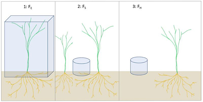
Figure 3. Schematic illustration of the different fluxes measured using the darkened chamber technique with either small or large chambers: whole ecosystem (F_E), soil (F_S), and heterotrophic (F_H) fluxes. The F_E chambers included 10 oat shoots.

Whole ecosystem flux, F_E

F_E was measured six times during the growing season, which lasted from 23 May to 14 August 2018. For the measurements, two large collars were installed in each plot, which had a surface area of 0.60 m × 0.60 m and rose to ~0.10 m above the soil surface. During sampling, these collars were mounted with white aluminum chambers 0.80 m in height with an inbuilt fan and a HOBO temperature logger.

Sampling was conducted by withdrawing 20 mL of air with a syringe every 1, 10, 20, 30, and 40 min after closing the chamber and inserting the gas sample in 10 mL glass vials (Labco Exetainer, Lampeter, Ceredigion, UK). The gas samples were analyzed using a gas chromatograph (7890A, Agilent Technologies, Santa Clara, CA, USA) equipped with a flame ionization detector and a methanizer for CO₂ and CH₄, and an electron capture detector for N₂O (Pihlatie et al., 2013). Kalu et al. (2022) described the F_E data measured from C0, C80, SprB, and WilB. This article reanalyzes the data, but with the addition of LimeS.

Heterotrophic and soil fluxes, F_H and F_S

The GHG fluxes were first measured on 8–9 May 2018. As this was done from bare soil before sowing, the collected data represented F_H. These measurements were conducted by placing an opaque chamber (0.20 m in height) on top of the large collars, as described previously. The GHG concentrations inside the closed chamber were then measured with a Gasmet Fourier transform infrared trace gas analyser DX4015 (Gasmet Technologies, Helsinki, Finland) by sucking air out and returning it back to the chamber with the flow rate of 2 L min⁻¹. The chamber also included a fan rotating at low speed to stir the air within the chamber. The measurement period was 5 min and therefore the increase in temperature was minor during the closure. The measurement was repeated three times at three different locations in each plot.

After the field was sown, six small collars (ø = 0.20 m) were permanently installed in each plot by inserting them to a depth of ~30–70 mm, which left ~80–120 mm above ground. Half of the collars were treated as F_S and half as F_H. The collars were removed before the harvest and afterwards placed in the middle of the harvested plots, which still included the oat stubble (Supplementary Figure 1C). Thereafter, flux measurements were carried out one to four times per month by closing the collars one by one with opaque Plexiglas and measuring the GHG concentrations inside the small air space with the Gasmet analyzer in a similar manner as with the large collars. Each measurement event lasted 3 min to avoid heating the air within the closed chamber. The small volume of chambers compared with the flowrate allowed efficient mixing of the chamber head space during these measurements due to lack of vegetation or other obstacles inside.

After plowing the soil in October 2018, we measured the GHG fluxes once during October and once during November from all treatments, except LimeS, using the large (0.60 m × 0.60 m) collars together with the opaque chamber. The shallower chambers were omitted because the soil surface was too rough for their installation. The closure time was again 5 min. In further analyses, the GHG fluxes after the harvest were handled as F_H due to a lack of notable living plant biomass.

Flux analyses

Prior to further data analysis, the development of CO₂ concentration during each measurement was evaluated visually. In the F_S and F_H measurements, the increase in the CO₂ concentration was observed to be unstable in 35 out of 1062 closures, indicating a leakage or other misbehavior of the measurement system. Those measurement events, including simultaneous CH₄ and N₂O fluxes, were then excluded from further analyses. The remaining data were used to calculate fluxes by linear fitting over GHG concentrations measured 30–150 s after the closure.

We analyzed all gases separately, but the data were also aggregated by pooling all GHG fluxes together after transforming both CH₄ and N₂O to CO₂eq according to their global warming potential using coefficients 25 and 298 for CH₄ and N₂O, respectively (IPCC, 2007).

Prior to other statistical analyses, all GHG variables were tested for normality (p > 0.05) using the Shapiro–Wilk test. Furthermore, both the N₂O and CO₂ fluxes were subjected to logarithmic transformation in order to meet the normality requirements. For the CH₄ fluxes, we removed outliers that were defined as data points that are located 1.5 times the interquartile range above the upper quartile and below the lower quartile. In practice, we used the boxplot function to remove 7 fluxes out of 139 as outliers before the analysis. The means of F_H in each plot were then compared among treatments using a two-way ANOVA with the treatment and the replicate block as factors in R (version 3.6.1, R Core Team, 2019), whereas with F_E, we used a two-way ANOVA with the treatment and date as factors.

Carbon balance

We calculated the carbon gain (C_gain) to the ecosystem from the atmosphere for each plot i as the difference between NPP (g C m⁻²) and heterotrophic respiration (RH, g C m⁻²), as follows

$\begin{array}{ll}{C}_{gain}=NP{P}_i-R{H}_i& (1)\end{array}$

We used the biomass production as NPP calculated by summing the biomass of roots, yield, and other above-ground biomass including weeds and by assuming the mean carbon content of dry biomass to be 50%.

We estimated RH using the momentary CO₂ emissions measurements from non-vegetated soil (F_H). First, we fitted for each plot i an empirical equation describing the temperature and moisture dependency, as follows:

$\begin{array}{ll}r{h}_i(t)={\left(1+{\left(\frac{1-RW{C}_i\left(t\right)}{\alpha }\right)}^v\right)}^{-1}{r}_{0,i}{Q}_{10,i}^{0.1T(t)}& (2)\end{array}$

where, t is day, T is daily mean soil temperature at 100 mm depth and α, r₀, and Q₁₀ are parameters obtained from the fitting. Measurements from all three collars in each plot were used to estimate the parameters for the plot. For v, we used a constant 11.27 according to Mäkelä et al. (2008). RWC is relative water content, calculated from the measured water content (M, m³ m⁻³) in the topmost soil layer, as

$\begin{array}{ll}RW{C}_i(t)=\frac{M_i(t)-WP}{FC-WP}& (3)\end{array}$

where, WP is the mean wilting point (0.15 m³ m⁻³) and FC denotes the field capacity for the topmost soil layer (0.28 m³ m⁻³) estimated from the measurements (Figure 4C). The daily rh_i values were then estimated using the measured soil moisture and temperature. Finally, the daily rh_i values were summed up to estimate heterotrophic respiration in each plot for the whole measurement season (197 days, 8 May−20 November), RH_i (g C m⁻²), as follows

$\begin{array}{ll}R{H}_i={{\displaystyle \sum }}_{t=1}^{197}r{h}_i(t)& (4)\end{array}$

In addition to the C_gain from the atmosphere, we calculated the change in the ecosystem carbon storage (ΔC_soil, g C m⁻²) as the difference between all the inputs and outputs, as follows

$\begin{array}{ll}{\Delta C}_{soil}=NPP-RH-Y& (5)\end{array}$

where, Y is the yield (g C m⁻²).

FIGURE 4

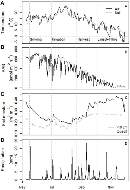
Figure 4. Daily mean air and soil temperature at a depth of 100 mm (A), photosynthetically active radiation (PAR) intensity (B), soil moisture at 0.10 m depth (C), and precipitation (D) measured throughout the campaign year, 2018. The station did not record the irrigation on 30 June, which was ~40–50 mm and which temporarily increased the soil moisture in the experimental plots. Panel (C) also includes the mean manual topsoil moisture (0–0.05 m) measurements.

We compared C_gain, ΔC_soil, RH, and NPP using a two-way ANOVA with the treatment and the replicate block as factors in R. We used the Shapiro–Wilk test prior to the analysis for testing normality (p > 0.05). In addition, we pooled all plots with amendments (LimeS, SprB, WilB) and compared those with the unamended ones (C0, C80N) using an independent 2-group t-test in R.

Results

General overview of the weather

In 2018, the snow melted at the study site in early April, which was still a relatively cool month before a more rapid temperature increase in early May. Thereafter, the site experienced very low precipitation in May, June, and July together with sunny weather and relatively high mean air temperatures (Figures 4A,B,D). The precipitation in June–August was 104 mm in Qvidja, i.e., even less than in Yltöinen (140 mm) that year and approximately half of the mean precipitation measured there during 1980–2010 (210 mm). This resulted in the soil drying out especially in late June and the first half of August (Figure 4C). The moisture content measured manually from the topsoil of each plot did not differ between treatments (not shown). Moreover, the seasonal changes observed in the manual measurements equaled the automatic measurements even though the overall moisture close to the soil surface (manual data) was somewhat less than in the deeper soil layer (automatic data) (Figure 4C).

During the dry and warm latter half of July, the control treatment C0 showed slightly higher soil temperatures than the other treatments (Supplementary Figure 2A). The soil temperature in replicate block 1 was 1–2 degrees less than that measured at the other blocks during June–July, but the differences between blocks evened out after harvest (Supplementary Figure 2B).

Soil structure and soil organic carbon

Overall, only WilB exhibited significant changes to total porosity (p = 0.034) and bulk density (ρ_bd) (p < 0.05), having significantly denser soil structure compared to the unamended (C80N) control (Table 2). However, SprB did exhibit ~16% larger PAW compared to C80N (p = 0.023) whereas LimeS and WilB tended to increase PAW by 9 and 10% on average. The increases in PAW had a strong positive correlation with the increase in SOC (R² = 0.72) whereby SprB, WilB, LimeS, and C80N had SOC contents of 3.54% (± 0.03), 2.97% (± 0.02), 2.62% (± 0.01), and 2.49% (± 0.02), respectively. Moreover, the SprB, WilB, and LimeS amended soil layer exhibited 10, 24, and 11% larger PAW compared to the deeper soil layer, whereas, with C80N, the difference between the two soil layers was negligible. This was in addition to the general trend, whereby the deeper soil layer had less large pores (>30 μm), and denser soil structure (p < 0.05) than the managed top soil layer. In addition, replicate block 1 exhibited significantly larger PAW (p < 0.05) when both the amended surface soil layer (0–0.05 m) as well as the deeper unamended soil layer (0.20–0.25 m) were included in the analysis. There was also a gradual increase in ρ_bd from one replicate block to the next (Table 2), whereby replicate block 3 had significantly denser structure (p < 0.05).

TABLE 2

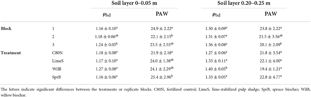
Table 2. Mean (± standard deviation) soil bulk density (ρ_bd, g cm⁻³) and plant available water (PAW, g g⁻¹) displayed as means of the three replicate blocks (N = 15) and treatments (N = 9) for the amended soil layer 0–0.05 m and deeper unamended soil layer 0.20–0.25 m.

Plant biomass and crop height

The height growth dynamics were generally similar among different treatments. However, the growth rate in SprB was increased in the later stages of development, whereas the non-fertilized control treatment (C0) lagged compared to the other treatments throughout the growing period (Figure 5). Consequently, SprB ended up having the tallest vegetation, whereas C0 had the shortest. Nevertheless, there were no statistical differences mainly due to the great variation between the different replicate blocks. The total mean plant biomass (± standard deviation) was 664 (± 364), 744 (± 266), 925 (± 252), 964 (± 265), and 1161 (± 210) g dry mass m⁻² in C0, C80N, LimeS, WilB, and SprB, respectively (Figure 6). In general, the largest biomass fractions and yield were recorded in the first replicate block and the smallest in the third block (not shown). The fraction consisting of leaves and stem was significantly larger in SprB than in the control treatments C0 or C80N. Other than this, none of the other biomass fractions nor the root/shoot ratio differed significantly between treatments due to large variation between the replicate blocks.

FIGURE 5

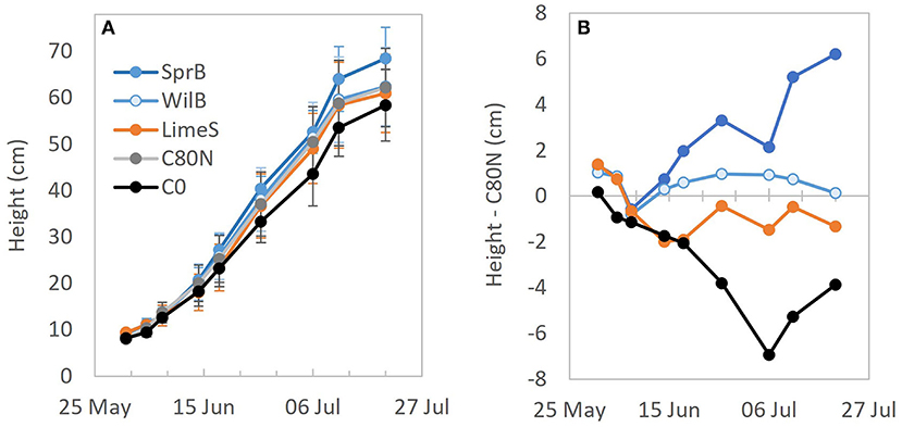
Figure 5. (A) Mean height of the oat in different treatment plots and (B) difference between the mean height in different treatment plots and the fertilized control plots (C80N) during the active lengthening period. C0, non-fertilized control; C80N, fertilized control; LimeS, lime-stabilized pulp sludge; SprB, spruce biochar; WilB, willow biochar.

FIGURE 6

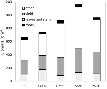
Figure 6. Mean yield, biomass of leaves and stem, roots, and other plants (weeds) as dry mass in the different treatment plots. Different letters indicate significant difference in the fluxes between the measured species (P < 0.05).

Gas exchange from bare soil

The F_H of CO₂ peaked in mid-May, right after sowing, and again in August–September, and was smaller during the dry period in June–July (Figure 7A). Increases in soil moisture, due to irrigation and precipitation along with a rather minor rain event on 20–21 June, led to a minor increase in heterotrophic CO₂ fluxes in early July. The largest mean F_H was measured from plots treated with LimeS and SprB (Figure 7B), but the differences between the treatments were not statistically significant. F_H of CO₂ was generally smaller than F_S from bare soil with surrounding plants, except on 31 July when the mean F_H clearly exceeded F_S in all treatments (Supplementary Figure 5).

FIGURE 7

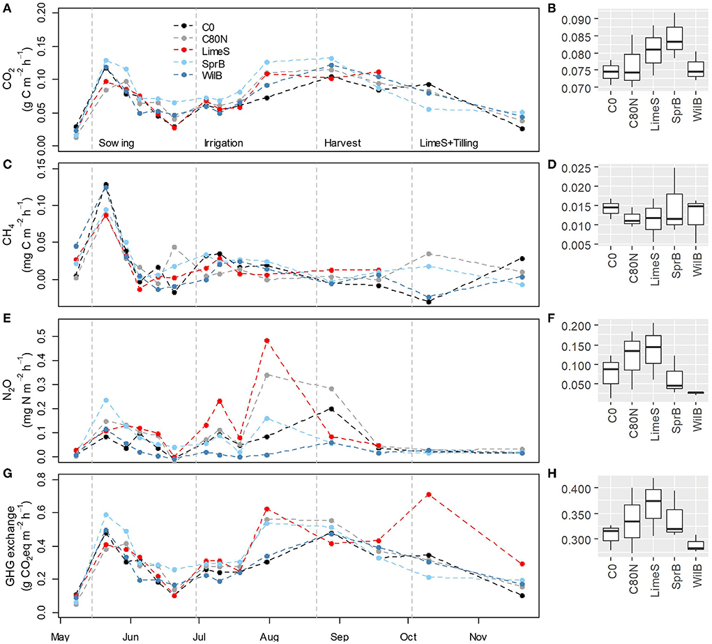
Figure 7. Left: Mean heterotrophic flux (F_H) for carbon dioxide (CO₂) (A), methane (CH₄) (C), nitrous oxide (N₂O) (E) and all greenhouse gases (GHGs) as CO₂ equivalents (G) in the different treatment plots measured from bare soil through the measurement campaign. Right: Mean F_H of CO₂ (B), CH₄ (D), N₂O (F) and GHG exchange (H) in the different treatment plots in May–September. Note the varying scale on the y-axis. Units in the panels on the right are the same as for the panels on the left. C0, non-fertilized control; C80N, fertilized control; LimeS, lime-stabilized pulp sludge; SprB, spruce biochar; WilB, willow biochar.

All treatments in the bare soil acted as CH₄ sources in mid-May, whereas later in the season the CH₄ exchange was close to zero (Figure 7C). The mean CH₄ exchange was comparable between the treatments (Figure 7D). N₂O emissions from bare soil fluctuated during the season showing highest peaks in late July, especially for the fertilized control (C80N) and LimeS treatments (Figure 7E). These treatments showed the largest mean N₂O emissions during the whole measurement period, whereas WilB showed the smallest (Figure 7F). When all GHGs were summed up as CO₂eq, LimeS showed the highest mean emissions and WilB the lowest (Figure 7H). Again, there were no statistically significant differences between treatments. There were no clear differences between F_H and F_S considering N₂O and CH₄ (Supplementary Figures 4, 5).

Gas exchange from vegetated soil (F_E)

The CO₂ fluxes were several times larger and CH₄ fluxes lower from the vegetated soil compared to the non-vegetated soil (Figures 7, 8). The largest CO₂ emissions from vegetated soil (F_E) were measured in July and the smallest in early June (Figure 8A). Overall, the only recorded statistically significant difference in CO₂ fluxes from the vegetated soil was between LimeS and SprB (Figure 8B). During the measurement period, the experimental plots fluctuated between small sinks and small sources of CH₄ (Figure 8C). WilB had the largest CH₄ sink but due to large variation, there were no statistical differences between the treatments (Figure 8D). Some of the C80N plots exhibited occasional peaks of N₂O, especially in late July and early August (Figure 8E). Overall, C80N and LimeS exhibited significantly greater N₂O emissions than WilB, but otherwise there were no significant differences between treatments (Figure 8F). Furthermore, there were no significant differences between the treatments when all GHGs were considered together as CO₂eq (not shown).

FIGURE 8

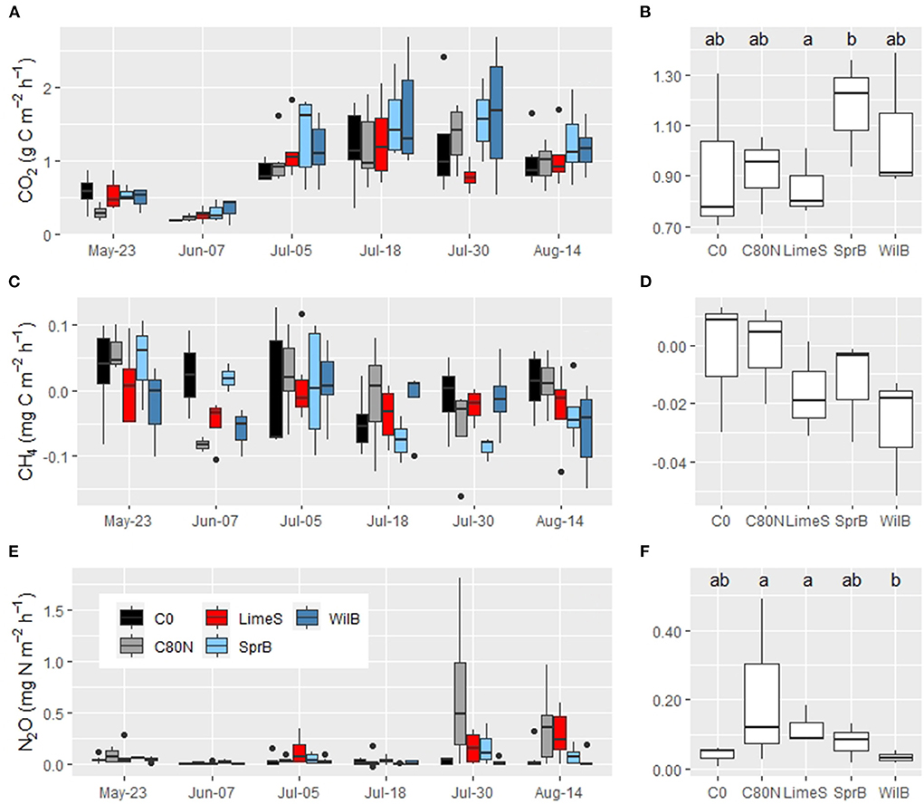
Figure 8. Left: (A,C,E) Box-and-whisker plots for whole ecosystem flux from vegetated soil in the different treatment plots during each measurement day. Right: (B,D,F) Means of all repetitions. Note the varying y-axis between the left and right panels. C0, non-fertilized control; C80N, fertilized control; LimeS, lime-stabilized pulp sludge; SprB, spruce biochar; WilB, willow biochar.

Carbon balance spanning over the growing season

The control treatment (C0) had the smallest, and SprB the largest, mean cumulative RH over the measurement campaign (8 May−20 November 2018, Figure 9A). Also, the C_gain represented by the difference between NPP and RH was most negative with C0 and the most positive with SprB (Figure 9B). In general, plots with soil amendments acted as a sink of atmospheric CO₂, whereas the plots without amendments had negative median values, indicating that they were sources of atmospheric CO₂ during the measurement campaign (Figure 9C). However, the soil carbon pool decreased in all treatment plots when accounting for the C loss in the form of yield (ΔC_soil, Figure 9C). Nevertheless, there were no significant differences between the treatments due to high variation between the replicates. Moreover, when all plots treated with soil amendments were pooled and compared against the unamended plots, the differences between RH, C_gain, and ΔC_soil values were close, but still not different, with p-values of 0.055, 0.061, and 0.060, respectively.

FIGURE 9

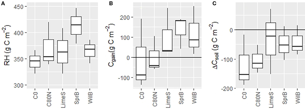
Figure 9. Box-and-whisker plots of heterotrophic respiration [RH, (A)], carbon gain between the ecosystem and the atmosphere as the difference between RH and biomass production (NPP) [C_gain, (B)], and the change in the soil carbon pool as the difference between the C_gain and the removed yield [ΔC_soil, (C)] during the campaign from 8 May to 20 November in 2018. Note the varying scale on the y-axes. C0, non-fertilized control; C80N, fertilized control; LimeS, lime-stabilized pulp sludge; SprB, spruce biochar; WilB, willow biochar.

Discussion

There is an urgent need to find management practices that decrease the negative climatic impact of traditional Nordic agriculture. Recent international studies with organic soil amendments have shown that they have generally favorable climatic impacts (Woolf et al., 2010; Griscom et al., 2017; Bai et al., 2019; Smith et al., 2020). However, studies in Finland have demonstrated only encouraging trends and many effects have remained statistically insignificant (e.g., Karhu et al., 2011; Soinne et al., 2020; Kalu et al., 2021). Our results continue this trend and show that the studied ligneous soil amendments had only moderate effects on plant biomass, soil water holding capacity and GHG exchange. However, the possible reasons for the lack of more significant differences arise from the low number of replicate blocks (three) accompanied by high variation in the studied variables due to possible spatial heterogeneity in the field. In addition, the campaign summer of 2018 was exceptionally warm and dry, which hindered both plant growth and soil microbial activity. This assumption is supported by the study by Heimsch et al. (2020) whose CO₂ exchange results from a nearby grassland at Qvidja indicated that the carbon uptake was clearly hindered by the dry and warm weather in 2018. Furthermore, the mean oat yield in 2018 (2.8 t ha⁻¹) was ~64% of the normal oat yield recorded in Varsinais-Suomi (Luke, 2020).

Soil physico-chemical properties and plant growth

Our first research question asked whether the soil amendments improved soil water holding capacity. Despite the natural, spatial differences in soil properties, the soil amendments were observed to benefit the soil structure. The benefits were most notable with SprB, which reduced the proportion of small pores and increased the number of large pores, resulting in an overall increase in PAW. This was attributed to increase in SOC, as there was a strong positive correlation between the increase of SOC and the increase of PAW. This indicates that the increase in SOC contributed to the increased water retention, as suggested by Foley and Cooperband (2002). Our conclusion is supported by the fact that PAW was increased only by the amendment treatments and not by the control treatment as illustrated by the comparison of the top soil layer (0–0.05 m) and the corresponding deeper unamended soil layer (0.20–0.25 m). Therefore, it is unlikely that soil management alone was the sole contributor to improving soil structure and water retention. It is also noteworthy that despite the higher response, the initial input of spruce biochar e.g., in total biomass and in dissolved nitrogen was lower than that of willow (Table 1) highlighting that other characteristics than just the amount applied to soil, play a key role degerming the impacts of soil amendments. Here, for example the stability of the amendment might have played a role as the SOC content was the highest in the spruce biochar treatment.

Our second research question asked whether the soil amendments improved net primary production. In our study, yield and total biomass were on average 28–75 and 24–56% higher in the amended plots than in the fertilized control plots, respectively. Additionally, some differences in root biomass tie in with the soil properties. By chance, all three replicate plots amended with WilB were in the south to south-west side of the field, which suffered from compaction as indicated by the increased bulk density. Consequently, WilB had the least root biomass, while the plots amended with LimeS were located on the opposite side of the field and had the most abundant root biomass. Indeed, there was a negative but insignificant relationship between the root biomass and the bulk density (not shown). Moreover, the differences in biomass growth between the replicate blocks coincided with the soil moisture properties and soil temperatures. Greater water holding capacity at replicate block 1 may partially explain the more abundant plant biomass, whereas taller vegetation as well as greater water content likely contributed to lesser soil temperatures (Rodskjer et al., 1989; Song et al., 2013). However, overall the only significant differences were found in the fraction of leaves and stem, which was larger in spruce biochar than in the control treatments. Therefore, our results are in line with extensive meta-analyses (Biederman and Harpole, 2013; Liu et al., 2013) that in Nordic case studies biochar application has yet to significantly increase biomass or yield (Tammeorg et al., 2014a,b; Soinne et al., 2020). Furthermore, our study reiterates the conclusion by Hakojärvi et al. (2013) that soil parameters alone are rarely enough to predict yield in case of high variation. Still, we conclude that the soil amendments provide long-term benefits to plant growth through improved soil conditions even if the benefits are not reflected directly by increases in yield (Phillips et al., 1997).

Greenhouse gas exchange

Our third research question examined whether soil amendments affect the GHG exchange between the ecosystem and the atmosphere. Our overall conclusion is that the CO₂ emissions from amended soils equaled, or at times exceeded, the unamended control, which we propose is a positive trend as it indicates that the treatments may have occasionally supported a more robust plant and soil activity during the unfavorable weather conditions. However, the CO₂ fluxes were inconsistent and the most pronounced heterotrophic CO₂ emissions were observed with LimeS and SprB, whereas the whole ecosystem CO₂ fluxes from LimeS were comparable with unamended treatments. In addition, the CO₂ fluxes from vegetated soil were many times larger than heterotrophic respiration, which is natural but may also be partly explained by the difference in the measurement method (Kohl et al., 2019). On the other hand, previous reports on GHG emissions in Finland show somewhat smaller overall CO₂ emissions from similar croplands located in southern Finland (Lohila et al., 2003; Regina and Alakukku, 2010; Karhu et al., 2011). We used linear fitting in the flux calculations even though it is criticized that the gas exchange must decrease during long closures as the concentration gradient between the chamber headspace and soil air decreases (Kutzbach et al., 2007). However, an exponential function would produce larger estimates than the linear regression function (Forbrich et al., 2010), whereas the latter is more stable overall, which we considered more fitting for examining treatment effects.

Significant CH₄ emissions require anaerobic conditions and the build-up of CO₂, which often develops only in water-saturated conditions (Conrad, 2007; Van Groenigen et al., 2011). Because of the low energy yield of methanogenesis, CH₄ emissions increase slowly and only after more favorable options have been exhausted (Lovley and Phillips, 1987). Therefore, it is unsurprising that CH₄ emissions were predominantly measured in May when the soil moisture was still high after the winter frost and melting snow. In addition, the sowing and tilling practices may have disturbed the soil, causing an outflow of accumulated gases from the soil system. A slight peak in CH₄ emissions was also recorded in July, after the soil moisture increased due to irrigation and a precipitation event, especially from non-vegetated soil. Throughout the rest of the growing season, CH₄ emissions fluctuated around zero without a clear trend and contributed little to the overall climatic effect of cultivation. However, the soil amendments seem to have a noticeable effect on the CH₄ exchange from vegetated soil, which were generally larger sinks of CH₄ even though the differences were non-significant. The reason for this remains unknown, but the results indicate soil hydrology as a major contributor, either by facilitating more abundant transpiring biomass and more even soil moisture conditions (Hiltbrunner et al., 2012), or through a liming effect. The latter explanation is supported by a recent meta-analysis on the effects of biochars on CH₄ emissions by Jeffery et al. (2016), which attributed pH as the predominant factor contributing to CH₄ exchange in non-flooded acidic soils during the growing period. However, it stated that the overall CH₄ exchange of non-flooded soils is outweighed by regularly flooded soils (i.e., paddy fields). In any case, the question remains, to what extent does CH₄ exchange during the cool and humid winter season contribute to the net CH₄ exchange of boreal agricultural soils?

The observed N₂O peaks followed the recorded irrigation and precipitation events during the growing season, reflecting the results from a parallel incubation (unpublished) experiment in which the C80N treatment exhibited significantly larger efflux of N₂O in response to rewetting than the ligneous fiber or biochar treatments. The occasional peaks may have been caused by enhanced microbial activity (Wagner-Riddle et al., 2008) or microbiological changes in respiration in response to changing redox conditions at soil microsites (Del Grosso et al., 2000; Fidel et al., 2017). Smaller peak emissions by the amendment treatments, especially in the WilB, may be due to greater volume of microsites and more stable soil conditions, which could in theory buffer sudden changes in soil moisture or aeration (Hagemann et al., 2016; Ribas et al., 2019). On the other hand, increased biomass growth decreases soil temperature and moisture compared to less-vegetated soil possibly further undercutting the conditions for N₂O production. However, the vegetation did not seem to have a clear effect on the N₂O fluxes in this study, as the emissions from vegetated and non-vegetated soil were generally very modest and equal in size. The differences in N₂O emissions measured from the bare soil may have been affected also by the natural variance in soil conditions, which may have been further influenced by the soil amendments, making it challenging to distinguish significant treatment effects. Our study lacked observations in midwinter and early spring whereas some studies report that in frozen soil areas, notable N₂O emissions occur during wintertime (Maljanen et al., 2007) or immediately after snowmelt and thawing of soil frost (Yanai et al., 2011; Risk et al., 2013). Therefore, those periods might be important when assessing the overall impact of soil amendments in the northern region.

Conclusions

Despite the lack of statistical differences, the numerous parallel trends with CO₂ and N₂O fluxes, plant biomass and soil properties indicate that the studied soil amendments had a favorable climatic impact. Among them, spruce biochar was the most beneficial for climate during the campaign as the decrease in the soil carbon storage was one of the lowest and it showed one of the lowest N₂O emissions. The N₂O emissions were clearly diminished by willow biochar as well, but it remains unclear to what extent this was caused by spatial variability. Additionally, lime-stabilized pulp sludge improved the soil quality and its effect on soil carbon pool was comparable with the studied biochars. However, as pulp sludge is considered to contain less stable carbon than the biochars, it is deemed less favorable in the long-term.

Further research is needed to conclusively characterize the specific effects of ligneous soil amendments on GHG exchange, soil structure and plant growth. However, together with other implications this study suggests that soil amendments in boreal agricultural sites have a favorable net climatic impact, as the amendments seem to improve soil properties, such as porosity and plant available water holding capacity even after two years of single application. It is debatable whether these changes will provide immediate benefits to crop production considering the quality of Finnish croplands. However, sustained use may help to maintain robust plant and soil activity during extreme weather events like droughts. We hope that in the future, better understanding of the soil processes will guide both the producers of soil amendments and policymakers into adopting more climate-smart management practices.

Data availability statement

The datasets presented in this study can be found in online repositories. The names of the repository/repositories and accession number(s) can be found below: https://doi.org/10.5281/zenodo.4401327.

Author contributions

LK, KP, and JH collected the empirical data. LK and KP were the main writers of the article. JH, MP, TL, JL, and AL supervised experimental design and contributed to the writing process producing the final version of the article. All authors approved the submitted version.

Funding

This study was supported by Sitra (Grant Hiilipilotti), the Strategic Research Council at the Academy of Finland (Grant Nos. 327214 and 327342) and Academy of Finland Flagship funding (Grant No. 337552).

Acknowledgments

We are grateful to Niina Ruoho and Tomi Mattila for their valuable help in field measurements, Elisa Vainio for the F_E calculations, Soilfood for the experimental set-up and yield measurements, and Qvidja farm owners and staff, especially Pekka Heikkinen and Jonathan Nylund for diverse practical assistance.

Conflict of interest

The authors declare that the research was conducted in the absence of any commercial or financial relationships that could be construed as a potential conflict of interest.

Publisher's note

All claims expressed in this article are solely those of the authors and do not necessarily represent those of their affiliated organizations, or those of the publisher, the editors and the reviewers. Any product that may be evaluated in this article, or claim that may be made by its manufacturer, is not guaranteed or endorsed by the publisher.

Supplementary material

The Supplementary Material for this article can be found online at: https://www.frontiersin.org/articles/10.3389/fsufs.2022.951518/full#supplementary-material

References

Abu-Hamdeh, N. H., and Reeder, R. C. (2000). Soil thermal conductivity effects of density, moisture, salt concentration, and organic matter. Soil Sci. Soc. Am. J. 64, 1285–1290. doi: 10.2136/sssaj2000.6441285x

CrossRef Full Text | Google Scholar

Bai, X., Huang, Y., Ren, W., Coyne, M., Jacinthe, P. A., Tao, B., et al. (2019). Responses of soil carbon sequestration to climate-smart agriculture practices: a meta-analysis. Glob. Change Biol. 25, 2591–2606. doi: 10.1111/gcb.14658

PubMed Abstract | CrossRef Full Text | Google Scholar

Beyer, L., Fründ, R., and Mueller, K. (1997). Short-term effects of a secondary paper mill sludge application on soil properties in a Psammentic Haplumbrept under cultivation. Sci. Total Environ. 197, 127–137.

Google Scholar

Biederman, L. A., and Harpole, W. S. (2013). Biochar and its effects on plant productivity and nutrient cycling: a meta-analysis. Glob. Change Biol. Bioenergy. 5, 202–214. doi: 10.1111/gcbb.12037

PubMed Abstract | CrossRef Full Text | Google Scholar

Bronick, C. J., and Lal, R. (2005). Soil structure and management: a review. Geoderma 124, 3–22. doi: 10.1016/j.geoderma.2004.03.005

CrossRef Full Text | Google Scholar

Chow, T. L., Rees, H. W., Fahmy, S. H., and Monteith, J. O. (2003). Effects of pulp fibre on soil physical properties and soil erosion under simulated rainfall. Can. J. Soil Sci. 83, 109–119. doi: 10.4141/S02-009

CrossRef Full Text | Google Scholar

Conrad, R. (2007). Microbial ecology of methanogens and methanotrophs. Adv. Agron. 96, 1–63. doi: 10.1016/S0065-2113(07)96005-8

CrossRef Full Text | Google Scholar

Dane, J. H., and Hopmans, J. W. (2002). “Soil water retention and storage - introduction,” in Methods of Soil Analysis. Part 4. Physical Methods. Soil Science Society of America Book Series No. 5, eds J. H. Dane and G. C. Topp (Madison, WI: Soil Science Society of America), 671–674.

Google Scholar

Del Grosso, S. J., Parton, W. J., Mosier, A. R., Ojima, D. S., Kulmala, A. E., and Phongpan, S. (2000). General model for N2O and N2 gas emissions from soils due to dentrification. Glob. Biogeochem. Cycles 14, 1045–1060. doi: 10.1029/1999GB001225

PubMed Abstract | CrossRef Full Text | Google Scholar

Fidel, R. B., Laird, D. A., and Parkin, T. B. (2017). Impact of six lignocellulosic biochars on C and N dynamics of two contrasting soils. Glob. Change Biol. Bioenergy 9, 1279–1291. doi: 10.1111/gcbb.12414

CrossRef Full Text | Google Scholar

Foley, B. J., and Cooperband, L. R. (2002). Paper mill residuals and compost effects on soil carbon and physical properties. J. Environ. Qual. 31, 2086–2095. doi: 10.2134/jeq2002.2086

PubMed Abstract | CrossRef Full Text | Google Scholar

Forbrich, I., Kutzbach, L., Hormann, A., and Wilmking, M. (2010). A comparison of linear and exponential regression for estimating diffusive CH4 fluxes by closed-chambers in peatlands. Soil Biol. Biochem. 42, 507–515. doi: 10.1016/j.soilbio.2009.12.004

CrossRef Full Text | Google Scholar

Griscom, B. W., Adams, J., Ellis, P. W., Houghton, R. A., Lomax, G., Miteva, D. A., et al. (2017). Natural climate solutions. Proc. Natl. Acad. Sci. U.S.A. 114, 11645–11650. doi: 10.1073/pnas.1710465114

PubMed Abstract | CrossRef Full Text | Google Scholar

Gupta, S. C., Dowdy, R. H., and Larson, W. E. (1977). Hydraulic and thermal properties of a sandy soil as influenced by incorporation of sewage sludge. Soil Sci. Soc. Am. J. 41, 601–605. doi: 10.2136/sssaj1977.03615995004100030035x

CrossRef Full Text | Google Scholar

Hagemann, N., Harter, J., and Behrens, S. (2016). “Elucidating the impacts of biochar applications on nitrogen cycling microbial communities,” in Biochar Application: Essential Soil Microbial Ecology, eds T. K. Ralebitso-Senior and C. H. Orr (Amsterdam: Elsevier), 163–198.

Google Scholar

Hakojärvi, M., Hautala, M., Ristolainen, A., and Alakukku, L. (2013). Yield variation of spring cereals in relation to selected soil physical properties on three clay soil fields. Eur. J. Agron. 49, 1–11. doi: 10.1016/j.eja.2013.03.003

CrossRef Full Text | Google Scholar

Heikkinen, J., Ketoja, E., Nuutinen, V., and Regina, K. (2013). Declining trend of carbon in Finnish cropland soils in 1974–2009. Glob. Change Biol. 19, 1456–1469. doi: 10.1111/gcb.12137

PubMed Abstract | CrossRef Full Text | Google Scholar

Heimsch, L., Lohila, A., Tuovinen, J.-P., Vekuri, H., Heinonsalo, J., et al. (2020). Carbon dioxide fluxes and carbon balance of an agricultural grassland in southern Finland. Biogeosciences 18, 3467–3483. doi: 10.5194/bg-18-3467-2021

CrossRef Full Text | Google Scholar

Hiltbrunner, D., Zimmermann, S., Karbin, S., Hagedorn, F., and Niklaus, P. A. (2012). Increasing soil methane sink along a 120-year afforestation chronosequence is driven by soil moisture. Glob. Change Biol. 18, 3664–3671. doi: 10.1111/j.1365-2486.2012.02798.x

CrossRef Full Text | Google Scholar

IPCC (2007). Climate Change 2007: The Physical Science Basis. Contribution of Working Group I to the Fourth Assessment Report of the Intergovernmental Panel on Climate Change. Cambridge University Press, Cambridge, UK and New York, NY, USA.

Google Scholar

Jeffery, S., Abalos, D., Prodana, M., Bastos, A. C., Van Groenigen, J. W., Hungate, B. A., et al. (2017). Biochar boosts tropical but not temperate crop yields. Environ. Res. Lett. 12:053001. doi: 10.1088/1748-9326/aa67bd

CrossRef Full Text | Google Scholar

Jeffery, S., Verheijen, F. G., Kammann, C., and Abalos, D. (2016). Biochar effects on methane emissions from soils: a meta-analysis. Soil Biol. Biochem. 101, 251–258. doi: 10.1016/j.soilbio.2016.07.021

CrossRef Full Text | Google Scholar

Kalu, S., Kulmala, L., Zrim, J., Peltokangas, K., Tammeorg, P., Rasa, K., et al. (2022). Potential of biochar to reduce greenhouse gas emissions and increase nitrogen use efficiency in boreal arable soils in the long-term. Front. Environ. 10:914766. doi: 10.3389/fenvs.2022.914766

CrossRef Full Text | Google Scholar

Kalu, S., Simojoki, A., Karhu, K., and Tammeorg, P. (2021). Long-term effects of softwood biochar on soil physical properties, greenhouse gas emissions and crop nutrient uptake in two contrasting boreal soils. Agric. Ecosyst. Environ. 316:107454. doi: 10.1016/j.agee.2021.107454

CrossRef Full Text | Google Scholar

Karhu, K., Mattila, T., Bergström, I., and Regina, K. (2011). Biochar addition to agricultural soil increased CH4 uptake and water holding capacity – results from a short-term pilot field study. Agric. Ecosyst. Environ. 140, 309–313. doi: 10.1016/j.agee.2010.12.005

CrossRef Full Text | Google Scholar

Kohl, L., Koskinen, M., Rissanen, K., Haikarainen, I., Polvinen, T., Hellén, H., et al. (2019). Technical note: interferences of volatile organic compounds (VOCs) on methane concentration measurements. Biogeosciences 16, 3319–3332. doi: 10.5194/bg-16-3319-2019

CrossRef Full Text | Google Scholar

Kutzbach, L., Schneider, J., Sachs, T., Giebels, M., Nykänen, H., Shurpali, N. J., et al. (2007). CO2 flux determination by closed-chamber methods can be seriously biased by inappropriate application of linear regression. Biogeosciences 4, 1005–1025. doi: 10.5194/bg-4-1005-2007

CrossRef Full Text | Google Scholar

Lehmann, J., Gaunt, J., and Rondon, M. (2006). Biochar sequestration in terrestrial ecosystems–a review. Mitig. Adapt. Strateg. Glob. Change 11, 403–427. doi: 10.1007/s11027-005-9006-5

CrossRef Full Text | Google Scholar

Lemola, R., Uusitalo, R., Hyväluoma, J., Sarvi, M., and Turtola, E. (2018). Suomen Peltojen Maalajit, Multavuus ja Fosforipitoisuus: Vuodet 1996–2000 ja 2005–2009. Luonnonvarakeskus, Helsinki, Finland. Available online at: https://jukuri.luke.fi/bitstream/handle/10024/541851/luke-luobio_17_2018.pdf?sequence=4andisAllowed=y (accessed May 06, 2022).

Google Scholar

Liu, X., Zhang, A., Ji, C., Joseph, S., Bian, R., Li, L., et al. (2013). Biochar's effect on crop productivity and the dependence on experimental conditions—a meta-analysis of literature data. Plant Soil 373, 583–594. doi: 10.1007/s11104-013-1806-x

CrossRef Full Text | Google Scholar

Lohila, A., Aurela, M., Regina, K., and Laurila, T. (2003). Soil and total ecosystem respiration in agricultural fields: effect of soil and crop type. Plant Soil 251, 303–317. doi: 10.1023/A:1023004205844

PubMed Abstract | CrossRef Full Text | Google Scholar

Lovley, D. R., and Phillips, E. J. (1987). Competitive mechanisms for inhibition of sulfate reduction and methane production in the zone of ferric iron reduction in sediments. Appl. Environ. Microbiol. 53, 2636–2641. doi: 10.1128/aem.53.11.2636-2641.1987

PubMed Abstract | CrossRef Full Text | Google Scholar

Luke (2020). Natural Resources Institute Finland, Statistics on Oat Yield in Finland, Varsinais-Suomi. Available online at: http://statdb.luke.fi/PXWeb/pxweb/fi/LUKE/LUKE__02%20Maatalous__04%20Tuotanto__14%20Satotilasto/01_Viljelykasvien_sato.px/?rxid=001bc7da-70f4-47c4-a6c2-c9100d8b50db (accessed May 06, 2022).

Google Scholar

Mäkelä, A, Pulkkinen, M., Kolari, P., Lagergren, F., Berbigier, P., Lindroth, A., et al. (2008). Developing an empirical model of stand GPP with the LUE approach: analysis of eddy covariance data at five contrasting conifer sites in Europe. Glob. Change Biol. 14, 92–108. doi: 10.1111/j.1365-2486.2007.01463.x

CrossRef Full Text | Google Scholar

Maljanen, M., Kohonen, A. R., Virkajärvi, P., and Martikainen, P. J. (2007). Fluxes and production of N2O, CO2 and CH4 in boreal agricultural soil during winter as affected by snow cover. Tellus B Chem. Phys. Meteorol. 59, 853–859. doi: 10.1111/j.1600-0889.2007.00304.x

CrossRef Full Text | Google Scholar

Matschullat, J., Reimann, C., Birke, M., dos Santos Carvalho, D., Albanese, S., Anderson, M., et al. (2018). GEMAS: CNS concentrations and C/N ratios in European agricultural soil. Sci. Total Environ. 627, 975–984. doi: 10.1016/j.scitotenv.2018.01.214

PubMed Abstract | CrossRef Full Text | Google Scholar

Millar, R. J., Fuglestvedt, J. S., Friedlingstein, P., Rogelj, J., Grubb, M. J., Matthews, H. D., et al. (2017). Emission budgets and pathways consistent with limiting warming to 1.5 C. Nat. Geosci. 10, 741–747. doi: 10.1038/ngeo3031

CrossRef Full Text | Google Scholar

Minasny, B., Malone, B. P., McBratney, A. B., Angers, D. A., Arrouays, D., Chambers, A., et al. (2017). Soil carbon 4 per mille. Geoderma 292, 59–86. doi: 10.1016/j.geoderma.2017.01.002

CrossRef Full Text | Google Scholar

Mokma, D. L., Yli-Halla, M., and Hartikainen, H. (2000). Soils in a young landscape on the coast of southern Finland. Agric. Food Sci. 9, 291–302. doi: 10.23986/afsci.5670

CrossRef Full Text | Google Scholar

Paustian, K., Lehmann, J., Ogle, S., Reay, D., Robertson, G. P., and Smith, P. (2016). Climate-smart soils. Nature 532, 49–57. doi: 10.1038/nature17174

PubMed Abstract | CrossRef Full Text | Google Scholar

Phillips, V. R., Kirkpatrick, N., Scotford, I. M., White, R. P., and Burton, R. G. (1997). The use of paper-mill sludges on agricultural land. Bioresour. Technol. 60, 73–80. doi: 10.1016/S0960-8524(97)00006-0

CrossRef Full Text | Google Scholar

Pihlatie, M. K., Christiansen, J. R., Aaltonen, H., Korhonen, J. F., Nordbo, A., Rasilo, T., et al. (2013). Comparison of static chambers to measure CH4 emissions from soils. Agric. For. Meteorol. 171, 124–136. doi: 10.1016/j.agrformet.2012.11.008

CrossRef Full Text | Google Scholar

Pirinen, P., Simola, H., Aalto, J., Kaukoranta, J., Karlsson, P., and Ruuhela, R. eds. (2012). Tilastoja Suomen ilmastosta 1981–2010 [Climatological statistics of Finland 1981–2010, in Finnsh]. Helsinki, Finland: Finnish Meteorological Institute, 83. Available online at: https://helda.helsinki.fi/handle/10138/35880 (accessed May 06, 2022).

Google Scholar

Price, G. W., and Voroney, R. P. (2007). Papermill biosolids effect on soil physical and chemical properties. J. Environ. Qual. 36, 1704–1714. doi: 10.2134/jeq2007.0043

PubMed Abstract | CrossRef Full Text | Google Scholar

R Core Team. (2019). R: A Language and Environment for Statistical Computing. R Foundation for Statistical Computing, Vienna, Austria. Available online at: https://www.R-project.org/

Google Scholar

Rasa, K., Pennanen, T., Peltoniemi, K., Velmala, S., Fritze, H., Kaseva, J., et al. (2021). Pulp and paper mill sludges decrease soil erodibility. J. Environ. Qual. 50, 172–184. doi: 10.1002/jeq2.20170

PubMed Abstract | CrossRef Full Text | Google Scholar

Rawls, W. J., Pachepsky, Y. A., Ritchie, J. C., Sobecki, T. M., and Bloodworth, H. (2003). Effect of soil organic carbon on soil water retention. Geoderma 116, 61–76. doi: 10.1016/S0016-7061(03)00094-6

CrossRef Full Text | Google Scholar

Regina, K., and Alakukku, L. (2010). Greenhouse gas fluxes in varying soils types under conventional and no-tillage practices. Soil Tillage Res. 109, 144–152. doi: 10.1016/j.still.2010.05.009

CrossRef Full Text | Google Scholar

Ribas, A., Mattana, S., Llurba, R., Debouk, H., Sebastia, M. T., and Domene, X. (2019). Biochar application and summer temperatures reduce N2O and enhance CH4 emissions in a Mediterranean agroecosystem: role of biologically-induced anoxic microsites. Sci. Total Environ. 685, 1075–1086. doi: 10.1016/j.scitotenv.2019.06.277

PubMed Abstract | CrossRef Full Text | Google Scholar

Risk, N., Snider, D., and Wagner-Riddle, C. (2013). Mechanisms leading to enhanced soil nitrous oxide fluxes induced by freeze–thaw cycles. Can. J. Soil Sci. 93, 401–414. doi: 10.4141/cjss2012-071

CrossRef Full Text | Google Scholar

Rodskjer, N., Tuvesson, M., and Wallsten, K. (1989). Soil temperature during the growth period in winter wheat, spring barley and ley compared with that under a bare soil surface at Ultuna, Sweden. Swed. J. Agric. Res. 19, 193–202.

Google Scholar

Roe, S., Streck, C., Obersteiner, M., Frank, S., Griscom, B., Drouet, L., et al. (2019). Contribution of the land sector to a 1.5°C world. Nat. Clim. Change 9, 817–828. doi: 10.1038/s41558-019-0591-9

CrossRef Full Text | Google Scholar

Rosenstock, T. S., Lamanna, C., Chesterman, S., Bell, P., Arslan, A., Richards, M., et al. (2016). The Scientific Basis of Climate-smart Agriculture: A Systematic Review Protocol. CCAFS Working Paper No. 138. Copenhagen, Denmark: CGIAR Research Program on Climate Change, Agriculture and Food Security (CCAFS). Available online at: https://hdl.handle.net/10568/70967 (accessed May 23, 2022).

Google Scholar

Smith, P. (2005). An overview of the permanence of soil organic carbon stocks: influence of direct human-induced, indirect and natural effects. Eur. J. Soil Sci. 56, 673–80. doi: 10.1111/j.1365-2389.2005.00708.x

CrossRef Full Text | Google Scholar

Smith, P., Calvin, K., Nkem, J., Campbell, D., Cherubini, F., Grassi, G., et al. (2020). Which practices co-deliver food security, climate change mitigation and adaptation, and combat land degradation and desertification? Glob. Change Biol. 26, 1532–1575. doi: 10.1111/gcb.14878

PubMed Abstract | CrossRef Full Text | Google Scholar

Soinne, H., Keskinen, R., Heikkinen, J., Hyväluoma, J., Uusitalo, R., Peltoniemi, K., et al. (2020). Are there environmental or agricultural benefits in using forest residue biochar in boreal agricultural clay soil? Sci. Total Environ. 731:138955. doi: 10.1016/j.scitotenv.2020.138955

PubMed Abstract | CrossRef Full Text | Google Scholar

Song, Y., Zhou, D., Zhang, H., Li, G., Jin, Y., and Li, Q. (2013). Effects of vegetation height and density on soil temperature variations. Chin. Sci. Bull. 58, 907–912. doi: 10.1007/s11434-012-5596-y

PubMed Abstract | CrossRef Full Text | Google Scholar

Tammeorg, P., Simojoki, A., Mäkelä, P., Stoddard, F. L., Alakukku, L., and Helenius, J. (2014a). Biochar application to a fertile sandy clay loam in boreal conditions: effects on soil properties and yield formation of wheat, turnip rape and faba bean. Plant Soil 374, 89–107. doi: 10.1007/s11104-013-1851-5

CrossRef Full Text | Google Scholar

Tammeorg, P., Simojoki, A., Mäkelä, P., Stoddard, F. L., Alakukku, L., and Helenius, J. (2014b). Short-term effects of biochar on soil properties and wheat yield formation with meat bone meal and inorganic fertiliser on a boreal loamy sand. Agric. Ecosyst. Environ. 191, 108–116. doi: 10.1016/j.agee.2014.01.007

CrossRef Full Text | Google Scholar

Tampio, E., Vainio, M., Virkkunen, E., Rahtola, M., and Heinonen, S. (2018). Opas kierrätyslannoitevalmisteiden tuottajille. Available online at: https://jukuri.luke.fi/bitstream/handle/10024/542240/luke-luobio_37_2018_2X.pdf?sequence=8andisAllowed=y (accessed May 06, 2022).

Google Scholar

Usowicz, B., Lipiec, J., Łukowski, M., Marczewski, W., and Usowicz, J. (2016). The effect of biochar application on thermal properties and albedo of loess soil under grassland and fallow. Soil Tillage Res. 164, 45–51. doi: 10.1016/j.still.2016.03.009

CrossRef Full Text | Google Scholar

Van Groenigen, K. J., Osenberg, C. W., and Hungate, B. A. (2011). Increased soil emissions of potent greenhouse gases under increased atmospheric CO2. Nature 475, 214–216. doi: 10.1038/nature10176

PubMed Abstract | CrossRef Full Text | Google Scholar

Wagner-Riddle, C., Hu, Q. C., Van Bochove, E., and Jayasundara, S. (2008). Linking nitrous oxide flux during spring thaw to nitrate denitrification in the soil profile. Soil Sci. Soc. Am. J. 72, 908–916. doi: 10.2136/sssaj2007.0353

CrossRef Full Text | Google Scholar

Wang, J., Xiong, Z., and Kuzyakov, Y. (2016). Biochar stability in soil: meta-analysis of decomposition and priming effects. Glob. Change Biol. Bioenergy 8, 512–523. doi: 10.1111/gcbb.12266

CrossRef Full Text | Google Scholar

Woolf, D., Amonette, J. E., Street-Perrott, F. A., Lehmann, J., and Joseph, S. (2010). Sustainable biochar to mitigate global climate change. Nat. Commun. 1, 1–9. doi: 10.1038/ncomms1053

PubMed Abstract | CrossRef Full Text | Google Scholar

Yanai, Y., Hirota, T., Iwata, Y., Nemoto, M., Nagata, O., and Koga, N. (2011). Accumulation of nitrous oxide and depletion of oxygen in seasonally frozen soils in northern Japan – snow cover manipulation experiments. Soil Biol. Biochem. 43, 1779–1786. doi: 10.1016/j.soilbio.2010.06.009

CrossRef Full Text | Google Scholar

Ylihalla, M., and Mokma, D. L. (2001). Soils in an agricultural landscape of Jokioinen, south-western Finland. Agri. Food Sci. 10, 33–43. doi: 10.23986/afsci.5677

CrossRef Full Text | Google Scholar

Yli-Halla, M., Mokma, D. L., and Alakukku, L. (2009). Evidence for the formation of Luvisols/Alfisols as a response to coupled pedogenic and anthropogenic influences in a clay soil in Finland. Agric. Food Sci. 18, 388–401. doi: 10.23986/afsci.5965

CrossRef Full Text | Google Scholar

Zibilske, L. M., Clapham, W. M., and Rourke, R. V. (2000). Multiple applications of paper mill sludge in an agricultural system: soil effects. J. Environ. Qual. 29, 1975–1981. doi: 10.2134/jeq2000.00472425002900060034x

CrossRef Full Text | Google Scholar

Zimmerman, A. R., Gao, B., and Ahn, M. Y. (2011). Positive and negative carbon mineralization priming effects among a variety of biochar-amended soils. Soil Biol. Biochem. 43, 1169–1179. doi: 10.1016/j.soilbio.2011.02.005

CrossRef Full Text | Google Scholar