Drivers of Animal Source Food Consumption: A Biophysical Approach

The contributions to energy and protein consumption of animal-source food (ASF) and its commodities bovine, pig, sheep and goat and poultry meat, fish and seafood, dairy products, and eggs were studied by multiple log-log-inverse regression of 1961–2017 consumption (MJ of energy, grams of protein) on income and year within country. The “year” variable implicitly captures time-dependent non-income factors such as prices, climate, agricultural area, urbanization, globalization, gender equality, religion. Fitting the latter six factors explicitly produced unrealistic results, likely due to insufficient within-country variation over time. All consumption patterns differed between countries, and changed over time; these differences and changes were related to income, but considerably more related to time-dependent non-income factors. Within-country estimates of the income elasticity (β) of total energy and protein consumption ranged from −1 to +1: when income increased by 1%, consumption changed by −1 to +1%. The corresponding estimates of the non-income time elasticity (γ) ranged from −0.05 to +0.05% per year: every year, adjusted for income, consumption changed by −0.05 to +0.05%. The β and γ estimates for the contribution of ASF to energy and protein consumption ranged twice as wide as these; those for the contributions of the individual commodities ranged at least three times as wide. The β and γ estimates for those commodities change considerably over time in many countries; their association to each other is very variable too, both between and within countries. Much of this variation takes place at the lower consumption levels. Considering all this, any attempt to forecast the consumption of animal source food (and particularly of its individual commodities) on a more detailed level than globally and on a longer term than a decade should include an income-independent time factor and be very careful with regard to the elasticity coefficients used.

Introduction

The sustainability of many production systems is internally antagonistic and the animal source food (ASF) production system with its antagonistic elements global food security, farmer livelihood, environmental load, animal welfare and safeguarded biodiversity is no exception (e.g., Knap, 2013; Capper, 2020). A balanced discussion of this sustainability issue will benefit from a clear description of ASF consumption patterns in various countries across the world over time, and from quantification of factors that change those patterns.

According to Timmer et al. (1983; pp. 57–58), “Engel's (1857) law refers to patterns of food expenditure relative to income, while Bennett's (1941) law refers to sources of food calories relative to income […]. The regular relationship between the two—that the average quality of food calories, measured by prices, rises with incomes—should probably be called Houthakker's (1957) law.” In other words, consumers tend to buy more expensive food calories when their income increases. An important intrinsic factor that makes food calories more expensive is that they derive from protein rather than carbohydates or fat; this is illustrated in Supplementary Figure 1 where the consumer price of food commodities, in Euros per Mcal of energy, shows a clear correlation to their protein-to-energy ratio.

Such consumption trends have been described in various forms and much detail by Juréen (1956); Hassan and Johnson (1977); Guo (2000); Regmi et al. (2001); Seale et al. (2003); Syrovátka (2004); Keyzer et al. (2005); Gale and Huang (2007); Pomboza and Mbaga (2007); FAO's (2009); Gandhi and Zhou (2010); Kumar et al. (2011); Muhammad et al. (2011); Robinson and Pozzi (2011); Neeteson-Van Nieuwenhoven et al. (2013); Bodirsky et al. (2015); Shyma (2016); Dolislager (2017); Ritchie and Roser (2017); Femenia (2019); Milford et al. (2019), and Le et al. (2020), among others. Most of these studies were done by economists. Not surprisingly, the default approach in the economy literature is to model consumption (often in terms of costs rather than quantity) in relation to income and price, regarding other influencing factors as effects to be adjusted for, e.g., age, education or religion at the micro consumer level; quality, availability or traditional preference at the commodity level; climate, urbanization or globalization at the macro societal level.

Key elements in such analyses are the regression coefficients of consumption on the predictor variables (e.g., income, price). It is useful to standardize these coefficients to a %-per- % scale, so that they can easily be compared across commodities and across predictor variables: a 1% change in income is associated with a certain % change in consumption. Such rescaling is implicitly done when the logarithm of income is regressed on the logarithm of the predictor variable; this gives the elasticity of consumption.

According to Timmer et al. (1983; p. 54), “frequently incomes and time are so strongly correlated that no separate [regression] coefficients are possible, and it takes a great deal of faith to attribute all time-related changes solely to income causation. But attributing it all to time is a profound expression of ignorance of the causal mechanisms at work.” For any non-economist, this leaves two obvious questions. First, how influential the income and non-income factors are, for the dynamics of consumption of food commodities, in the various countries in the world; second, what such patterns look like in terms of actual consumption rather than its cost: a biophysical rather than economical approach. This is what I try to quantify here. I also attempt to translate the associated econometric terminology into terms less confusing for readers educated in the life sciences.

Materials and Methods

Food consumption and income data are analyzed here with a statistical approach similar to those of Bodirsky et al. (2015) who included a “year” variable in their model to implicitly account for time-variant non-income factors, Muhammad et al. (2011) who analyzed global data on a within-country basis, and Gale and Huang (2007) who applied a log-log-inverse model to allow the regression estimates to change with income. All three these approaches are included in the analysis, and consumption is quantified not economically in terms of financial expenditure, but biophysically in terms of the contribution of a given commodity to total energy or protein consumption; this is done for each of eight ASF commodities, longitudinally across the 1961–2017 period.

Countries and Population Size

In the graphs in the Results section, countries with interesting attributes are identified by the ISO-3166 alpha-3 codes (from AFG for Afghanistan to ZWE for Zimbabwe, and mostly very obvious) listed at www.iso.org/iso-3166-country-codes.html. The various countries are grouped into 10 socio-economic regions, from west to east: the Anglo-Saxon world, Latin America, Sahara and Sahel, southern Africa, Europe, the former Soviet Union, West Asia and Bangladesh, South Asia, Centrally Planned Asia, and South-East Asia—color-coded in inset maps in those graphs. This grouping was modified from Lotze-Campen et al. (2008); OSISA (2009), and Femenia (2019) in an attempt to find a reasonable combination of geographical, economical, cultural and ecological elements with an influence on dietary patterns. This grouping does not play any role in the statistical analysis of the data, which will take place on a by-country level; it is only used to summarize the results of those analyses in hopefully manageable and informative clusters.

Human population size in 235 countries has been recorded since 1950, and published by UN (2019). These values are used for scaling purposes.

Data on the countries that make up the former Soviet Union were available only from 1992 to 2016.

Food Consumption

The supply of foodstuffs available for human consumption across the world has been published by FAO since 1961. “The total quantity of foodstuffs produced in a country, added to the total quantity imported and adjusted to any change in stocks that may have occurred, […] gives the supply available during that period. On the utilization side, a distinction is made between the quantities exported, fed to livestock, used for seed, put to manufacture for food use and non-food uses, losses during storage and transportation, and food supplies available for human consumption” (www.fao.org/faostat/en/#data/FBS). Such country-level values are converted to a per caput basis, and expressed in terms of (i) quantity, (ii) protein content, (iii) fat content, and (iv) metabolizable energy (caloric value, derived from protein, fat and carbohydrate content). The conversion factors are in Annex I of FAO (2001).

The resulting data from 1961 to 2013 is in www.fao.org/faostat/en/#data/CL (for ASF) and www.fao.org/faostat/en/#data/CC (for plant-source food: PSF). Data from 2014 and further is in www.fao.org/faostat/en/#data/FBS. The focus is here on the ASF commodities bovine meat, pig meat, sheep and goat meat, poultry meat, fish and seafood, dairy products, and eggs.

Note that this data does not quantify actual consumption, but the supply available for it on an as purchased basis; the difference is due to (i) inedible parts such as bones (see Westhoek et al., 2015) and to (ii) wastage at the consumer level (Gustavsson et al., 2011; Alexander et al., 2017; Lopez Barrera and Hertel, 2020).

Kearney (2010) gives much useful discussion of this FAO data, its background and its interpretation.

These consumption data have distinct autocorrelation structures: 1,170 of 1,341 country-commodity consumption patterns in the data show significant first-order autocorrelations across the time period.

Income

A wide variety of economic parameters across the world has been published by the World Bank, for some countries since 1960 and for most since 1990. This includes various versions of the Gross Domestic Product (GDP), i.e., “the sum of gross value added by all resident producers in the economy, plus any product taxes, and minus any subsidies not included in the value of the products” in a country. Such country-level quantities are converted to a per caput basis, and expressed in terms of constant (or real) international dollars (int$, following the Geary-Khamis method: unstats.un.org/unsd/methods/icp/ipc7_htm.htm) using Purchasing Power Parity rates—this adjusts for inflation over time, and makes the data comparable across countries. The World Bank converts to 2017-int$ in its NY.GDP.PCAP.PP.KD series, available at databank.worldbank.org/source/world-development-indicators#advancedDownloadOptions.

An alternative series is made available by the Maddison Project Database (Bolt et al., 2018). This includes estimates that go back a long time and run up to 2016, expressed in constant (or real) 2011-int$. This data is available at www.rug.nl/ggdc/historicaldevelopment/maddison/releases/maddison-project-database-2018.

For presenting long time trends, the main appeal of the Maddison data is that it covers the whole FAO foodstuffs supply recording period from 1961, whereas much of the World Bank data starts only around 1990. The full Maddison data set was used for the GDP values of 1961–2016 and the 2017 values of the World Bank series were appended to it as follows.

Linear regression of the Maddison values for 2016 (MAD₂₀₁₆) on the World Bank values for 2016 (WBK₂₀₁₆) produces a correlation at +0.986. This holds for 144 of 150 countries; the other six (Kuwait, Luxembourg, Norway, Singapore, Qatar and the United Arab Emirates; less than 0.4% of the 2016 world population) have some of the highest GDP values in the Maddison series, and show significant deviations from this regression (see also Bolt et al., 2018, p. 39). Hence they are not processed further and their trends end in 2016. For each of the other 144 countries, its World Bank value for 2017 was rescaled as WBK₂₀₁₇ × MAD₂₀₁₆/WBK₂₀₁₆.

General Patterns of Consumption in Relation to Income

To make it easier to compare my results to the literature, it is useful to relate consumption patterns to income only—before we engage in more elaborate statistical analyses.

Illustrating the first quotation from Timmer et al. (1983) in the Introduction section (“the average quality of food calories, measured by prices, rises with incomes”), Figure 1 shows the 1961–2017 time trend of inflation-adjusted income in the various countries (Figure 1A), the corresponding time trends of protein and energy consumption (Figures 1B,D), and these two consumption variables as they relate to income (Figures 1C,E). Income increases significantly over time for 140 out of 150 countries; only Kuwait, Qatar and the United Arab Emirates show significantly (P < 0.1) decreasing income over time, starting from suspiciously high early levels. Not surprisingly, protein and energy consumption show time trends similar to this; hence, relating them to income itself (Figures 1C,E) produces convincing patterns of increasing consumption with increasing income, with tentative plateaus at 3.0–3.5 Mcal ME per day and 90–110 g protein per day. Those convincing patterns may be misleading due to the collinearity of income with time.

FIGURE 1

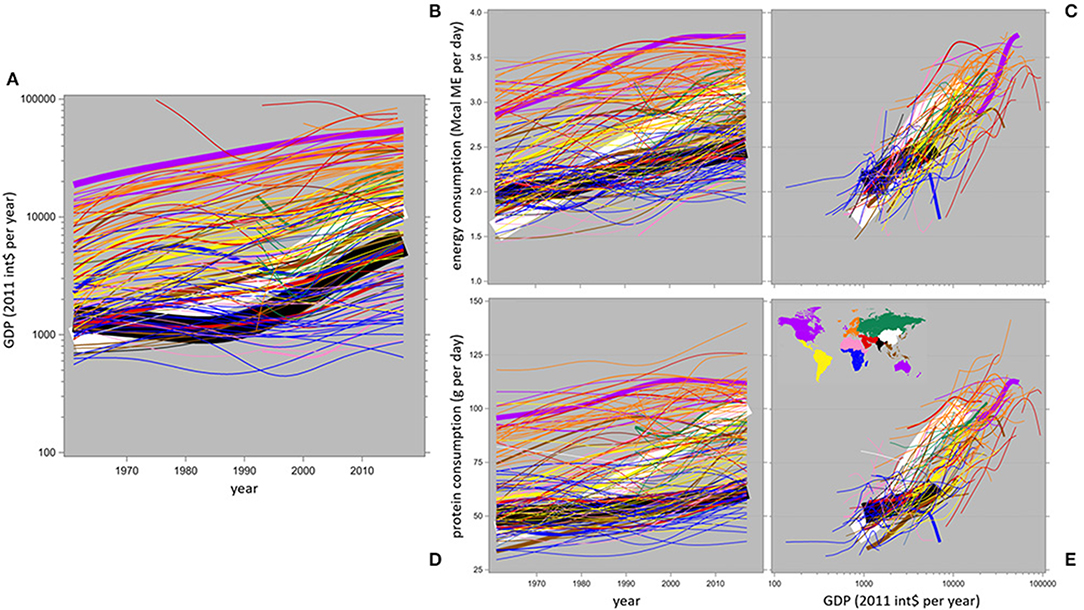
Figure 1. Country-specific spline interpolation plots (estimated by SAS-procedure TRANSREG with a smoothing factor sm = 60) of inflation-adjusted income in relation to time (A), of energy and protein consumption in relation to time (B,D), and of energy and protein consumption in relation to income unadjusted for other factors (C,E). The width of each line reflects the country's population size in 2016. Note that the income axes are logarithmic.

Both these plateaus are somewhat higher than the generally recommended consumption levels. For a moderately active individual with the global average adult body weight of 62 kg (Walpole et al., 2012), the consumption recommendations of FAO (2004; Table 5.4–5.7) work out as 2.7 Mcal ME per day, and those of Wu (2016; Table 5) as 60–100 g protein per day, with a “safe upper limit” at 220 g per day.

The energy consumption trends in Figure 1 show some subtle differences from the protein consumption ones; these can be made clearer by the ratio of daily protein-to-energy consumption as it is shown in relation to income in Figure 2—in total, and separately for ASF and PSF. An alternative would be to plot these ratios in relation to time but that produced poorer resolution, similar to Figure 1B vs. Figure 1C.

FIGURE 2

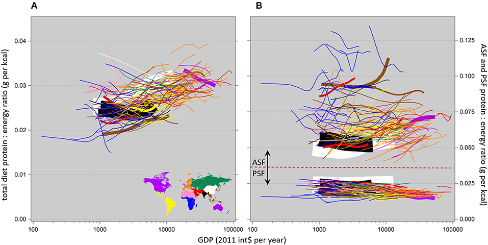
Figure 2. Country-specific spline interpolation plots of the ratio of daily protein-to-energy consumption in relation to income, not adjusted for any non-income factors, in the total diet (A) and in the ASF- and PSF-based parts of the diet (B). The width of each line reflects the country's population size in 2016. Note that the x-axis is logarithmic and the y-axes differ in scale.

To place these protein-to-energy ratio values into perspective, Table 1 shows some of the 190 commodities listed in Annex I of FAO (2001), with their conversion factors that were used to calculate these ratios. The trends shown here for PSF and ASF are functionally due to increasing protein content and decreasing fat content, respectively. The trends in Figure 2 represent some average of those 190 commodity values, dependent on the local dietary mix; the relevant issue here is that this local dietary mix changes over time and/or with income, as described by Popkin's (1993, 1995) nutrition transition.

TABLE 1

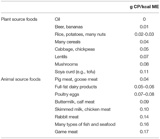
Table 1. Crude protein to metabolizable energy ratio in various food commodities, from FAO (2001, Annex I).

Figure 2A shows that in most countries, the protein content of the whole diet apparently increases with increasing income; this is due to at least three factors.

First, the protein content of the PSF-based part of the diet in many countries apparently decreases slowly but steadily with increasing income, as in the lower plot in Figure 2B.

Second, the protein content of the ASF-based part of the diet in many countries apparently increases with increasing income although there is considerable variation here, particularly in Africa and South-East Asia; see the upper plot in Figure 2B.

Third, the ASF-based proportion of the diet apparently increases with increasing income, at the expense of the PSF-based proportion. In an attempt to improve upon the informativeness of FAO's (2009) famous Figure 3, the ASF-sourced proportions of total daily energy and protein consumption are shown here in relation to income in Figure 3; obviously, the complement is due to PSF. As per above, the ASF-based proportion of the diet is apparently increasing with increasing income, in terms of both energy and protein consumption. This appears to plateau around 20–30% of energy consumption and 50–60% of protein consumption being ASF-based, with much more between-country variation for energy than for protein.

FIGURE 3

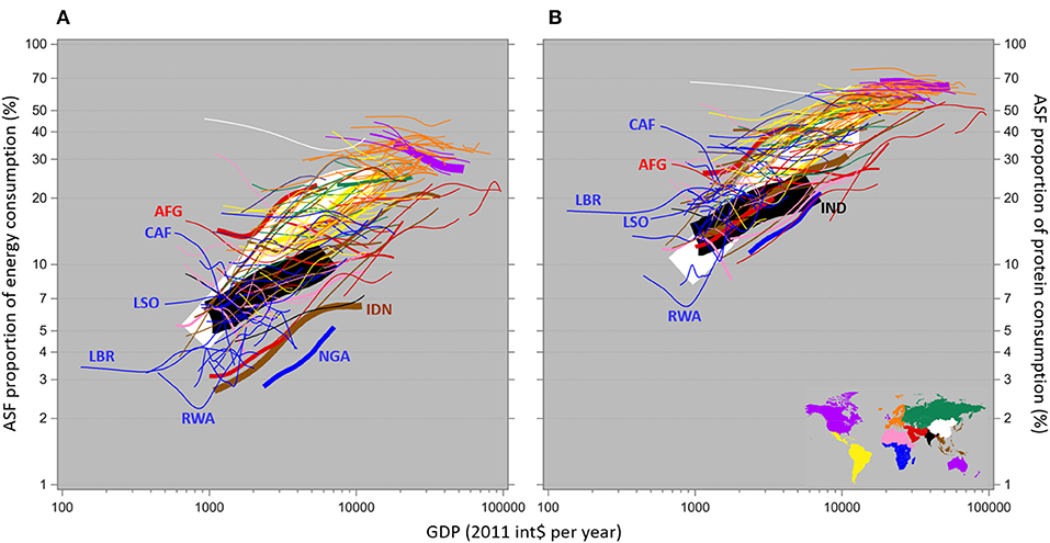
Figure 3. Country-specific spline interpolation plots of the proportions of daily energy (A) and protein (B) consumption that are based on animal source foods, in relation to income and not adjusted for any non-income factors. The width of each line reflects the country's population size in 2016. Note that both axes are logarithmic.

Price

The typical economic demand analysis describes consumption as a function of income and price, usually also including the effect of substitution of one commodity for other ones when prices change; a good example is Muhammad et al. (2011).

Producer (farm-gate) prices of a wide array of foodstuffs have been published by FAO across the world since 1991, at http://www.fao.org/faostat/en/#data/PP. This website notes that “retail prices […] are typically very poor proxies for producer prices.” Since this also applies the other way around and this study focuses on consumption as opposed to production, I chose to ignore these producer price data.

Global consumer prices of various food commodities vary strongly between countries, as is shown by their frequency distributions for eight commodities in Supplementary Figure 2. Vegetables and fruit are three to four times more expensive than globally in a few countries (Japan and some Caribbean islands) and less than half as expensive in several more (mostly in Africa and Asia) with everyone else in between; the standard deviations across countries (averaged across the 2 years) are 63 and 51 index points, respectively. The prices of the other commodities vary less widely, with standard deviations between 30 and 43 index points. None of these distributions show significant differences between 2011 and 2017 (0.10 < P < 0.86), but each of these prices shows significant (P < 0.0001) re-ranking of countries between the years, particularly at the higher price levels.

The price of food roughly follows overall inflation in most countries, as is shown by the global time trends of the food consumer price index vs. the general consumer price index in Supplementary Figure 3, but food prices increased faster than overall inflation in 122 of these 175 countries, significantly so (P < 0.05) in 100 of them. Food prices increased more slowly than overall inflation in the other 53 countries, significantly so in 34 of them. These patterns are not significantly influenced by country GDP (P = 0.27) nor by socio-economic region (P > 0.09).

Hence the inflation- and PPP-adjusted prices of ASF and PSF commodities vary strongly among countries at any given time, and they show different time trends among countries. Given this, it makes no sense to analyze long-term data of consumption of particular commodities in many countries, in terms of price indicators that were estimated for a few specific years only, or were averaged across commodities or across countries (such as the various FAO food commodity price indexes as they are available from www.fao.org/worldfoodsituation/en).

Statistical Analysis

The statistical analysis is based on the classical Engel equation (Stone, 1954): consumption = α · (income)^β1 so that ln(consumption) = β₀ + β₁ · ln(income), where β₀ = ln(α) and ln(·) is the natural logarithm.

Note that the regression coefficient of a linear regression model y = α + β · x quantifies the additive change in y associated with additive change in x (β = dy / dx). When such a linear system relates consumption to income, β is expressed in g/d per $. A one-dollar increase in income then leads to a predicted increase in consumption of β g/d, and this is assumed to apply to initial income levels across the whole range of 1,000–100,000 $ per year. This is clearly unrealistic.

By contrast, the regression coefficient β of a logarithmic model such as the one of above is multiplicative: it quantifies the proportional change in y (some percentage of the initial consumption level) as it relates to proportional change in x (e.g., 1% of the initial income level), i.e., $\frac{\text{dy}}{\text{y}}/\frac{\text{dx}}{\text{x}}$ , expressed in % per %. In econometric terminology this is the income elasticity of consumption. The absolute (as opposed to proportional) income-related change in consumption is the marginal propensity to consume (MPC = $\frac{\text{dy}}{\text{dx}}$ ), in contrast to the average propensity to consume (APC = $\frac{\text{y}}{\text{x}}$ ). The elasticity is β = MPC / APC $=\frac{\text{dy}}{\text{dx}}/\frac{\text{y}}{\text{x}}=\frac{\text{dy}}{\text{y}}/\frac{\text{dx}}{\text{x}}$, as above. From there, dy $=\beta ·\frac{\text{y}}{\text{x}}·$dx : for any value of β, a one-dollar increase in income (dx) leads to an absolute increase in consumption (dy) that is lower at higher initial income levels (x) and at lower initial consumption levels (y). This is much more realistic than the linear approach of above, but the outcome is less intuitive to interpret quantitatively; see point 1 in Supplementary Material 3 for more mathematical properties.

The econometric demand studies in the literature apply various types of regression model: apart from the linear (y = α + β · x) and double-logarithmic (ln(y) = α + β · ln(x)) ones of above, there are the inverse (y = α + β / x), semi-logarithmic (y = α + β · ln(x)), log-inverse (ln(y) = α + β / x), and log-log-inverse (ln(y) = α + β₁ · ln(x) + β₂ / x) models. The latter model goes back to Goreux (1960) and was more recently applied by Gale and Huang (2007):

$\begin{array}{l}\text{ln}(\text{consumption})={\beta }_0+{\beta }_1·\text{ln}(\text{income})\\ +{\beta }_2·(1/\text{income})& (1)\end{array}$

As above, $\beta =\frac{\text{dy}}{\text{dx}}/\frac{\text{y}}{\text{x}}$ and the derivative is now $\frac{\text{dy}}{\text{dx}}=({\beta }_1-{\beta }_2·\frac{1}{\text{x}})·\frac{\text{y}}{\text{x}}$, i.e., the income elasticity β is a function of income itself; see point 2 in Supplementary Material 3 for more mathematical properties. This approach allows the elasticity to change with changing income: a very useful attribute. This is an extremely multicollinear system: ln(x) and 1/x will be strongly correlated for any realistic range of x. Indeed, in this data the correlation over time between ln(income) and (1 / income) ranges from −0.92 for South Korea to −0.9997 for Belgium. The actual estimates of β₁ and β₂ are then best ignored as such, focusing instead on their more interesting combination $\beta ={\beta }_1-{\beta }_2·\frac{1}{\text{income}}$.

The analyses are conducted with extensions of this equation of the form:

$\begin{array}{l}\text{ln}({\text{consumption}}_{\text{i}})={\beta }_{0\text{i}}+{\beta }_{1\text{i}}·\text{ln}({\text{income}}_{\text{i}})+\\ {\beta }_{2\text{i}}·(1/{\text{income}}_{\text{i}})+{\beta }_{3\text{i}}·\text{ln}({\text{x}}_{3\text{i}})+\dots \\ +{\beta }_{8\text{i}}·\text{ln}({\text{x}}_{8\text{i}})& (2)\end{array}$

…where subscript i denotes the countries. The variables x₃ to x₈ represent, for each country, non-income factors that can be expected to influence consumption: the OAI climate index of annual rainfall and temperature, the agricultural area per caput, the urbanization proportion, the KOF globalization index, the WBL gender equality index, and the proportion of Islam adherence. These factors are described in detail in Supplementary Material 1.

The parameter β₀ is the intercept; β₁ and β₂ are regression coefficients of consumption on income; β₃ to β₈ are regression coefficients of consumption on each of the independent variables. Note that price effects are not included here, as reasoned in section Price.

As was partly illustrated in Figure 1, many of these factors (and also income) are systematically increasing or decreasing over time (i.e., they are trending), which again leads to multicollinearity in the system. The within-country linear correlations among the trending independent variables, averaged across countries, range from +0.49 (income vs. urbanization) to +0.85 (globalization vs. gender equality). Multicollinearity in regression analysis can be dealt with in several ways.

First, much of the issue is due to implicit parametric assumptions about the form of the relationship between the dependent variable and each independent one; this can be resolved by a nonparametric approach (e.g., McNamee, 2005), for example by modeling some of the independent variables with splines which can be done with SAS procedure GAMPL (SAS Institute, 2018).

Second, by transforming the collinear set of independent variables into an orthogonal set via principal component analysis, and regressing the dependent variable on the most informative components via a partial least squares approach (e.g., Fekedulegn et al., 2002), for example with SAS procedure PLS (SAS Institute, 2018).

Third, by removing some of the independent variables from the statistical model via a covariate selection approach such as ridge regression or its derivatives (see Blommaert et al., 2014), to optimize the statistical model's informativeness vs. parsimoniousness via penalization of the model's R² or likelihood for the number of parameters to be estimated. With only six additional covariates as in model (3) an all possible subsets approach is feasible, following Fernandez (2007) and Huang and Zhu (2015).

Analyses of this data with any of these methods did not produce convincing results; either the multicollinearity was not sufficiently resolved, or too many subsets produced nonsense estimates or failed to converge. This is in stark contrast to Milford et al. (2019) who obtained credible estimates for the effects of similar factors in an across-country analysis of meat and ruminant meat consumption. Apparently these factors do not vary sufficiently over time within country to provide meaningful information for this type of analysis.

Instead, inspired by models (3) and (7) of Bodirsky et al. (2015), all non-income factors (including prices, implicitly) were replaced by a single time factor (year), as follows:

$\begin{array}{l}\text{ln}({\text{consumption}}_{\text{i}})=({\alpha }_{1\text{i}}+{\alpha }_{2\text{i}}·\text{year})\\ +({\beta }_{1\text{i}}+{\gamma }_{1\text{i}}·\text{year})·\text{ln}({\text{income}}_{\text{i}})\\ +({\beta }_{2\text{i}}+{\gamma }_{2\text{i}}·\text{year})·(1/{\text{income}}_{\text{i}})& (\mathrm{3a})\end{array}$

…so that the intercept α₁ and the regression coefficients β₁ and β₂ of model (1) are made time-dependent by extending them with a “year” variable that carries its own coefficients α₂, γ₁ and γ₂.

This can be rearranged as:

$\begin{array}{l}\text{ln}({\text{consumption}}_{\text{i}})={\alpha }_{1\text{i}}+{\alpha }_{2\text{i}}·\text{year}\\ +{\beta }_{1\text{i}}·\text{ln}({\text{income}}_{\text{i}})+{\beta }_{2\text{i}}·(1/{\text{income}}_{\text{i}})\\ +{\gamma }_{1\text{i}}·\text{year}·\text{ln}({\text{income}}_{\text{i}})\\ +{\gamma }_{2\text{i}}·\text{year}·(1/{\text{income}}_{\text{i}})& (\mathrm{3b})\end{array}$

…which features an intercept, a “year” covariate, the two income-derived variables, and as the novel element the interaction terms of these with “year.”

Subscript i denotes the countries again.

Model (3) leads to final time-adjusted income elasticities of consumption of the form:

$\begin{array}{l}\beta =\left({\beta }_1-\frac{{\beta }_2}{\text{income}}\right)\\ +\left({\gamma }_1-\frac{{\gamma }_2}{\text{income}}\right)·\text{year}\end{array}$

…which is the proportional change in consumption due to proportional change in income (% per %), adjusted for simultaneous change in other time-related factors.

Likewise, model (3) leads to final income-adjusted time elasticities of the form:

$\begin{array}{l}\gamma ={\alpha }_2+{\gamma }_1·ln(\text{income})\\ +\frac{{\gamma }_2}{\text{income}}\end{array}$

…which is the proportional change in consumption due to a unit change in time (% per year), adjusted for simultaneous change in income. Note that this change in time comes with implicit changes in non-income factors such as price, the variables x₃ to x₈ of model (2), and any other time-variant factors.

See point 3 in Supplementary Material 3 for derivations and mathematical properties of β and γ.

Model (3) was applied using a REML approach in SAS procedure GLIMMIX (SAS Institute, 2018), modeling the residual terms with a first-order autoregressive covariance system with country as the subject. This was done for total energy and protein consumption, and for their proportions due to ASF and due to the invidual commodities bovine meat, pig meat, sheep and goat meat, poultry meat, fish and seafood, dairy products, and eggs. The relevant SAS program code is in Supplementary Material 5.

GLIMMIX reports the model's likelihood and its derived Information Criteria such as Akaike's AIC. These are useful for discriminating between different models of the same data, typically via likelihood ratio tests. The Akaike Weights of Burnham and Anderson (2004) and Wagenmakers and Farrell (2004) were used to quantify the contribution in model (3) of the non-income time factor over and above income. From the AIC values of the full model (AIC_full) and its income-only submodel (AIC_income), the probability that the submodel is more appropriate (informative and parsimonious) is given by the Akaike Weight AICW:

$\begin{array}{l}\text{AICW}=\frac{\text{relL}}{1+\text{ relL}}\text{with relative likelihoodrelL}\\ =e^{-1/2.}\Delta \text{AIC and }\Delta \text{AIC}={\text{AIC}}_{\text{full}}-{\text{AIC}}_{\text{income}}.\end{array}$

These Information Criteria do not quantify how much variation in the data is explained by a given model as the classical coefficient of determination R² does, and GLIMMIX does not report R². An adjusted version of Kvalseth's (1985) pseudo-R² was calculated post-hoc, penalized for the number of independent variables (Theil, 1961):

$\begin{array}{ll}{\text{R}}_{\text{adj}}^2=1-\frac{\text{N}-1}{\text{N}-\text{k}-1}·\frac{\sum {\left(\text{y}-\widehat{\text{y}}\right)}^2}{\sum {\left(\text{y}-\stackrel{\overline{\text{y}}}{}\right)}^2}& (4)\end{array}$

…where y denotes the observations of the dependent variable, $\stackrel{\overline{\text{y}}}{}$ is their overall mean, $\widehat{\text{y}}$ denotes the predicted values, k is the number of independent variables, and N is the number of observations, i.e., years per country (N ≤ 56). This was done for the full model (3) (k = 6) and for its income-only submodel (k = 4).

In the final term of equation (4), the numerator is the model's residual sum of squares. It is scaled to the overall variance of the observations by the denominator, which represents the sum of squared residuals for a “model” that is simply the average response, ignoring any independent variables (k = 0). Linear regression cannot perform worse than $\widehat{\text{y}}=\stackrel{\overline{\text{y}}}{}$, so R² ≥ 0 for such models; but non-linear regression with an inappropriate model can lead to negative pseudo-R² values (Alexander et al., 2015).

The sampling variances (and from those, the standard errors) of the β and γ estimates, var(β) and var(γ), can be derived analytically from the sampling variances and covariances of the β₁, β₂, γ₁ and γ₂ estimates (see Supplementary Material 2); some of the estimated covariances are so large (due to multicollinearity once more) that these var(β) and var(γ) estimates are negative for most of the commodity-country combinations. To avoid this, the β and γ estimates were bootstrapped (Efron and Tibshirani, 1986) by resampling the residuals from model (3), with replacement and stratified by country, and running the GLIMMIX regression again; this was done 500 times and the variances of the 500 resulting β and γ estimates serve as approximations of var(β) and var(γ), for each commodity-country-year combination. The relevant SAS program code is in Supplementary Material 5.

Results

Model Fit

The non-income time factor plays an important role in the predictive performance of model (3), over and above income; this is quantified in Figure 4.

FIGURE 4

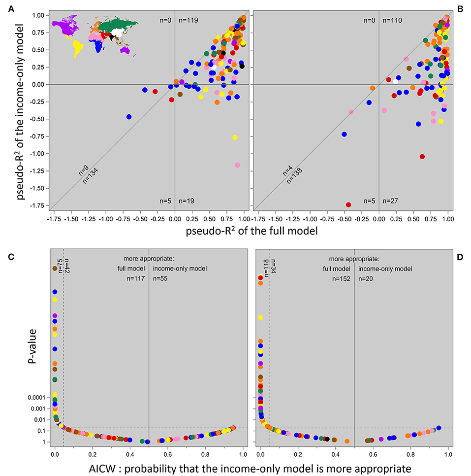
Figure 4. Penalized pseudo-R² values of our full model (3) and its income-only submodel, for the contributions of animal source foods (A) and poultry meat (B) to protein consumption. Akaike Weights and the likelihood ratio test P-values of their underlying ΔAIC [i.e., $P({\chi }_2^2>\Delta AIC$)] of our full model (3) vs. its income-only submodel, for the contributions of fish and seafood (C) and poultry meat (D) to protein consumption. Note that the y-axes in (C,D) are logarithmic and reversed, i.e., datapoints further to the top represent more strongly significant differences between the models. The horizontal reference lines in (C,D) indicate the most strongly significant cases where the income-only model is more appropriate; the dotted vertical reference lines indicate the AICW values where the full model achieves that same significance. Each datapoint represents a country.

The penalized pseudo-R² values for the full model (3) and for its income-only submodel are shown for the contributions of ASF (Figure 4A) and poultry meat (Figure 4B) to protein consumption; the patterns for the other commodities are somewhere between these two. Datapoints above the diagonal are cases where the income-only submodel is more appropriate (informative and parsimonious) than the full model; this holds for 3–6% of the countries (Figure 4A: six Southern African countries, the Dominican Republic, Ukraine, Serbia and Slovakia; Figure 4B: Chad, Israel, Italy and Croatia). Another relevant comparison is between the number of datapoints to the left of the vertical reference line vs. below the horizontal one, i.e., where the data are exceedingly poorly fitted by the full model (4% of the countries; Figure 4A: Afghanistan, Lebanon, Angola, Liberia and Malawi; Figure 4B: Croatia, Lebanon, Chad, Mozambique and Nigeria) or by the income-only submodel (17–22% of the countries; in Figures 4A,B: 25 countries in Africa, nine in Latin America, seven in West Asia, four in Europe, Cambodia, the Philippines and Kyrgyzstan).

The Akaike Weights and likelihood ratio test P-values of their underlying ΔAIC values for the full model (3) and for its income-only submodel are shown for the contributions of fish and seafood and poultry meat to protein consumption in Figures 4C,D; the patterns for the other commodities are somewhere between these two. For the countries where the income-only model is the more appropriate one (AICW > 0.5), the P-values range from 0.054 to 1; about as many countries where the full model is more appropriate fall in that same non-significant range, and substantially more show a much stronger statistical significance. These patterns are not significantly related to the actual contribution of any commodity to protein consumption (P > 0.34); the full model is significantly more appropriate for the ASF contribution to protein consumption in countries with a higher protein consumption (P = 0.018), for the bovine meat contribution in countries with a larger population size (P = 0.015), and for the contribution of eggs in countries with a larger population size, a higher protein consumption, and a lower GDP (P < 0.024). Apart from that, no meaningful connections to any variable in the data could be detected.

Properties of the Elasticity Estimates

The bootstrapped Student's t-values (i.e., the estimate divided by its bootstrapped standard error) of the β and γ estimates for total protein consumption, and for the contributions of ASF and poultry meat to it, are in Figure 5; these are the variables with the most extreme elasticity estimates. The t-values for the other commodities are included in Supplementary Material 4.

FIGURE 5

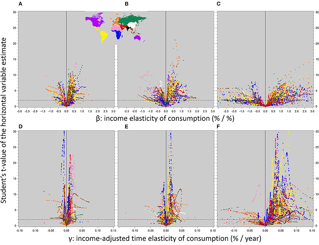
Figure 5. The β and γ elasticity estimates of total protein consumption (A,D) and of the contributions of animal source food (B,E) and poultry meat (C,F) to it on the x-axes, and the absolute values of their bootstrapped Student's t-values on the y-axes. The dotted horizontal reference lines indicate the 95% significance level: estimates below these lines do not differ significantly from zero. Each datapoint represents a country-year-combination.

Clearly, model (3) represents a demanding statistical exercise: across all the commodity contributions to protein consumption, only 27–41% of the β estimates, and only 48–71% of the γ estimates, turn out to be significantly different from zero (P < 0.05), almost irrespective of their magnitude. There are no clear relationships between these significance levels and the actual levels of consumption: the correlations between the t-value and actual consumption range from −0.04 to +0.05 for β, and from −0.15 to +0.01 for γ; this comes back in the Results and Discussion sections.

The β and γ estimates in Figure 5 are much more narrowly distributed for total protein consumption and for its ASF component than for its poultry meat (and, not shown here, the other commodities') component; the estimates as such are dealt with below. More to the point at this stage, on average across country-year combinations the t-values of the γ estimates are between 8.7 (for fish and seafood) and 25 (for poultry meat) times as high as those of their associated β estimates. This repeats the R²- and AIC-related inference of above: the income-adjusted time factor plays an important role in the predictive performance of model (3), over and above income.

Energy and Protein Consumption

The average per caput energy and protein consumption in 1967, 1992; and 2016 in the socio-economic regions and worldwide are listed in the first half of Table 2; this summarizes the country-level patterns in Figures 1B,D. During this period, global average consumption increased linearly from 2.26 to 2.91 Mcal ME per day and from 61 to 82 g protein per day; most regions experienced a similar rate of development with the exception of the former Soviet Union where the average increase was very slow and Centrally Planned Asia (CPA) where it was very strong.

TABLE 2

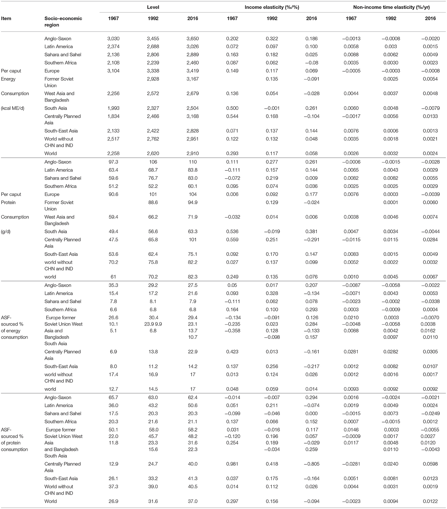
Table 2. Time trends of energy and protein consumption and of the contribution made to these by animal source food (ASF), and of their estimated income elasticities (β) and non-income time elasticities (γ). CHN: China, IND: India.

These country-level averages would suggest that a large proportion of the world population has now reached, or is close to reaching, the abovementioned recommended consumption levels of 2.7 Mcal ME and 60–100 g protein per day. However, any within-country variation in consumption remains hidden here; considering that more than a third of the adult populations of Africa and of South and South-East Asia were overweight in 2013 (Ng et al., 2014), without doubt undernutrition is still frequent in these regions.

Table 2 also shows the regional averages of the within-country regression coefficients of energy or protein consumption on income and on time, i.e., the β and γ elasticity estimates from model (3). During this period, the global average income elasticities of energy and protein consumption (β) both decreased from around +0.3 to less than +0.1 and this global pattern is much dominated by China and India: in the rest of the world the energy β coefficient decreases much less (from +0.1 to +0.05) and the protein β coefficient actually increases from +0.03 to +0.1.

At the same time, the global average non-income time elasticity (γ) of energy consumption is essentially constant: the net effect of an increase in CPA and a similar decrease in South Asia, with a slight average decrease in the rest of the world. The global average γ coefficient of protein consumption shows a linear increase over time, dominated by a strong increase in CPA that is dampened by reductions in Europe, South Asia, and South-East Asia.

The overall pattern is clearly one of substantial regional variation, and the regional average values in Table 2 do not even represent the considerable within-region variation among countries, which is shown in Figure 6. The elasticities are shown here not in relation to the independent regression variables time or income, but in relation to the actual consumption level of the country-year combination that they were estimated for, inspired by Masterman and Viscusi (2018), their Figure 2B). In the horizontal dimension, a datapoint further to the right represents more daily per caput consumption in that country in that year. In the vertical dimension, a datapoint further to the top represents a stronger increase of consumption with increasing income (β) or other time-associated factors (γ) in that country in that year.

FIGURE 6

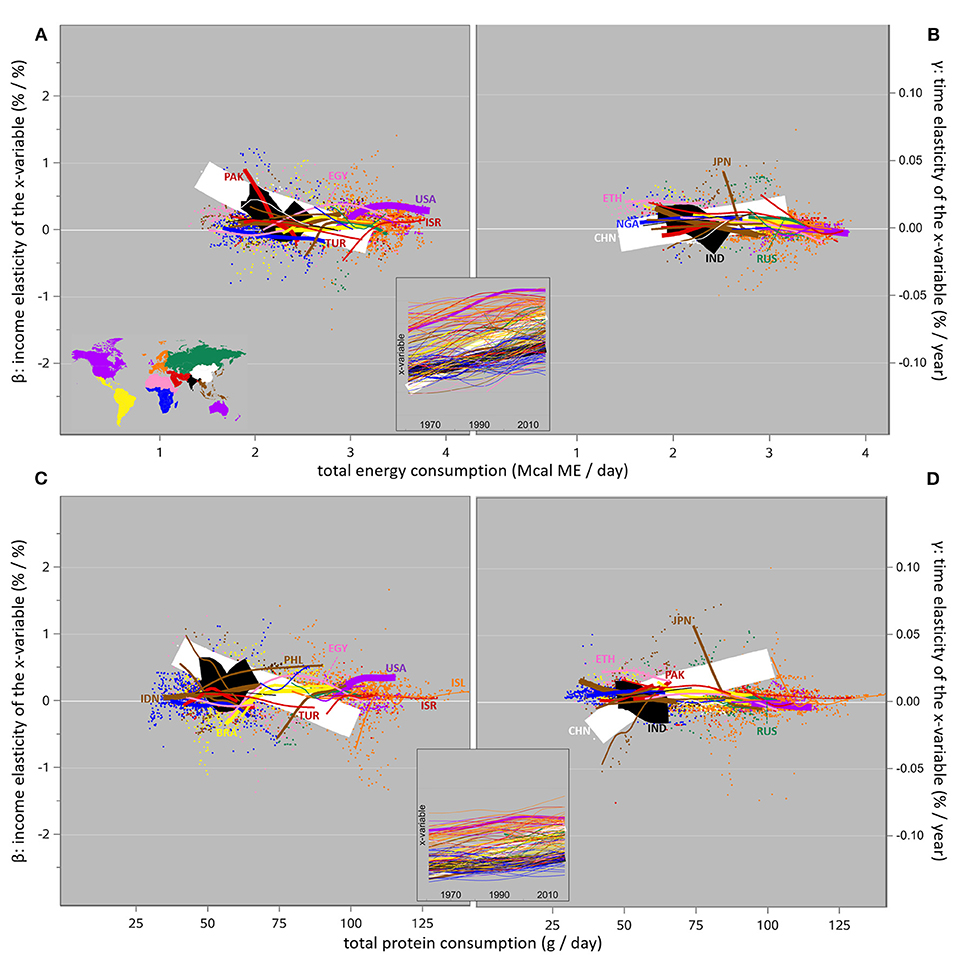
Figure 6. Regression coefficients of the logarithm of total daily energy (A,B) or protein (C,D) consumption on the logarithm of annual income (β: the income elasticity, adjusted for time-related non-income effects), and on time and its associated non-income effects (γ: the time elasticity, adjusted for income effects), from 1961 to 2017. Both estimates change over time and are shown in relation to each year's actual consumption on the x-axes. Each datapoint represents a country-year combination. The trendlines are spline interpolation plots (see Figure 3 for details) across time for the most populous countries, and for the countries with the highest consumption levels, covering >76% of the world population. The insets show the time trends of consumption (i.e. the x-variables of the main graphs), as in Figure 3B. The width of each trendline reflects the country's population size in 2016.

These graphs are visually dominated by the trendlines for China, where at first glance the β and γ trends seem to simply mirror each other. That would suggest an inability of the regression model to separate the two effects, in line with the second quotation from Timmer et al. (1983) in the Introduction section (“frequently incomes and time are so strongly correlated that no separate [regression] coefficients are possible”). However, the β estimates for energy and protein consumption in China decrease from clearly positive values until they reach zero at consumption levels of 2.84 Mcal/d and 84 g/d, respectively, and then continue toward more negative values. The associated γ estimates increase from clearly negative values to reach zero at the much lower consumption levels of 1.89 Mcal/d and 52 g/d, respectively. Hence between protein consumption levels of 52 and 84 g/d (i.e., over more than half the total trajectory from 40 to 101 g/d), β and γ for China are both positive.

In summary, between 1961 and 2017 a majority across the world increased their daily energy and protein consumption. This was influenced by changes in income, as shown in Figures 6A,C; and often it was more strongly influenced by non-income factors, as shown in Figures 6B,D. These effects of income (positive β estimates) and of other factors (positive γ estimates) vary strongly between countries and over time.

Animal and Plant Source Food Consumption

The second half of Table 2 shows the average ASF contributions to energy and protein consumption in 1967, 1992; and 2016 in the socio-economic regions and worldwide. During this period, the global average of those contributions increased from 13 to 17% of energy consumption, and from 27 to 37% of protein consumption. Most of this increase took place in CPA and Latin America; the Anglo-Saxon world and the former Soviet Union show reductions.

Table 2 also shows the regional averages of the within-country regression coefficients of the ASF contributions to energy and protein consumption on income and on time, i.e., the β and γ elasticity estimates from model (3). During this period, the global average income elasticity (β) of the ASF contribution to energy consumption changed very little, but the underlying regional changes are very strong, dominated again by almost perfectly mirrored patterns for CPA (a strong decrease) and South Asia (a similarly strong increase). The associated global average β coefficient for protein consumption decreased from +0.3 to −0.1: the net effect of a decrease from +1 to −0.8 in CPA and much smaller changes in either direction elsewhere.

At the same time, the global average non-income time elasticities (γ) of the ASF contributions to energy and protein consumption changed very little, again with variable underlying regional changes: (i) the γ coefficient for protein in CPA increased from −0.03 to +0.06 while its energy counterpart did not change at all, (ii) both γ coefficients in the Sahara and Sahel region decreased from zero to −0.03 during the second half of the reporting period, and (iii) the rest of the world was relatively stable in this respect, mostly at close-to-zero levels.

As in the previous section, the ASF contributions to energy and protein consumption and also their β and γ coefficients show much regional variation; the within-region variation among countries is just as large and is shown in Figure 7: between 1961 and 2017, most countries steadily increased the ASF-derived proportions of their energy and protein consumption, irrespective of any changes in income (positive γ estimates). The corresponding income-related changes (the β estimates) show complex patterns that seem to converge to zero with increasing ASF consumption, as much from positive as from negative β levels; as mentioned in connection with Figure 5 (section Properties of the Elasticity Estimates), the β estimates are not systematically less (or more) accurate at the lower consumption levels, so this is likely a true saturation effect .

FIGURE 7

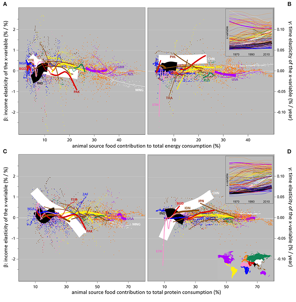
Figure 7. Regression coefficients of the logarithm of the proportions of daily energy (A,B) or protein (C,D) consumption that are based on animal source food, on the logarithm of annual income (β: the income elasticity, adjusted for time-related non-income effects), and on time and its associated non-income effects (γ: the time elasticity, adjusted for income effects), from 1961 to 2017. Note that the x-axes show the actual contribution% levels, not time or income; the time trends of the x-variable are shown in the insets. See Figure 6 for details on the lay-out.

For illustration of the β-γ interplay, consider in Figure 7 the ASF-based energy consumption patterns for China, where the non-income elasticity γ is positive during the whole time period, and the income elasticity β moves from +0.8 to zero with increasing consumption levels, until 1994 when 15% of the energy consumption was sourced from ASF ingredients, after which the β estimates stay slightly negative. The net result is a steady but plateauing increase in ASF consumption over time (see the inset), and this increase is less and less income-driven. This holds even more strongly for ASF-based protein consumption in China.

Hence it seems that over time, and (independent from that) with increasing income, most people consume more energy and protein and many replace part of the PSF in their diet by ASF, most notably the protein-rich ingredients (e.g., pulses and soya). Hence the role of PSF in the worldwide diet shifts gradually toward the provision of energy (mainly from carbohydrates and fat) rather than of protein. The role of ASF in the diet shifts into the opposite direction, most likely because the global consumption of animal fat (a strong contributor to ASF energy) is slowly decreasing. Le et al. (2020) give more detail on these trends. Most importantly, there are considerable differences among socio-economic regions and among countries in the interplay between the income and non-income effects on the dynamics of these consumption patterns.

Animal Source Food Commodities

The abovementioned changes in ASF consumption involve different commodities in different parts of the world; this is quantified in more detail here for the contributions of dairy products, fish and seafood, pig meat, bovine meat, poultry meat, eggs, and sheep and goat meat—for the sake of brevity, their contribution to protein consumption only. The average contributions in 1967, 1992; and 2016 in the various socio-economic regions and worldwide are in Table 3, together with their β and γ elasticity estimates from model (3).

TABLE 3

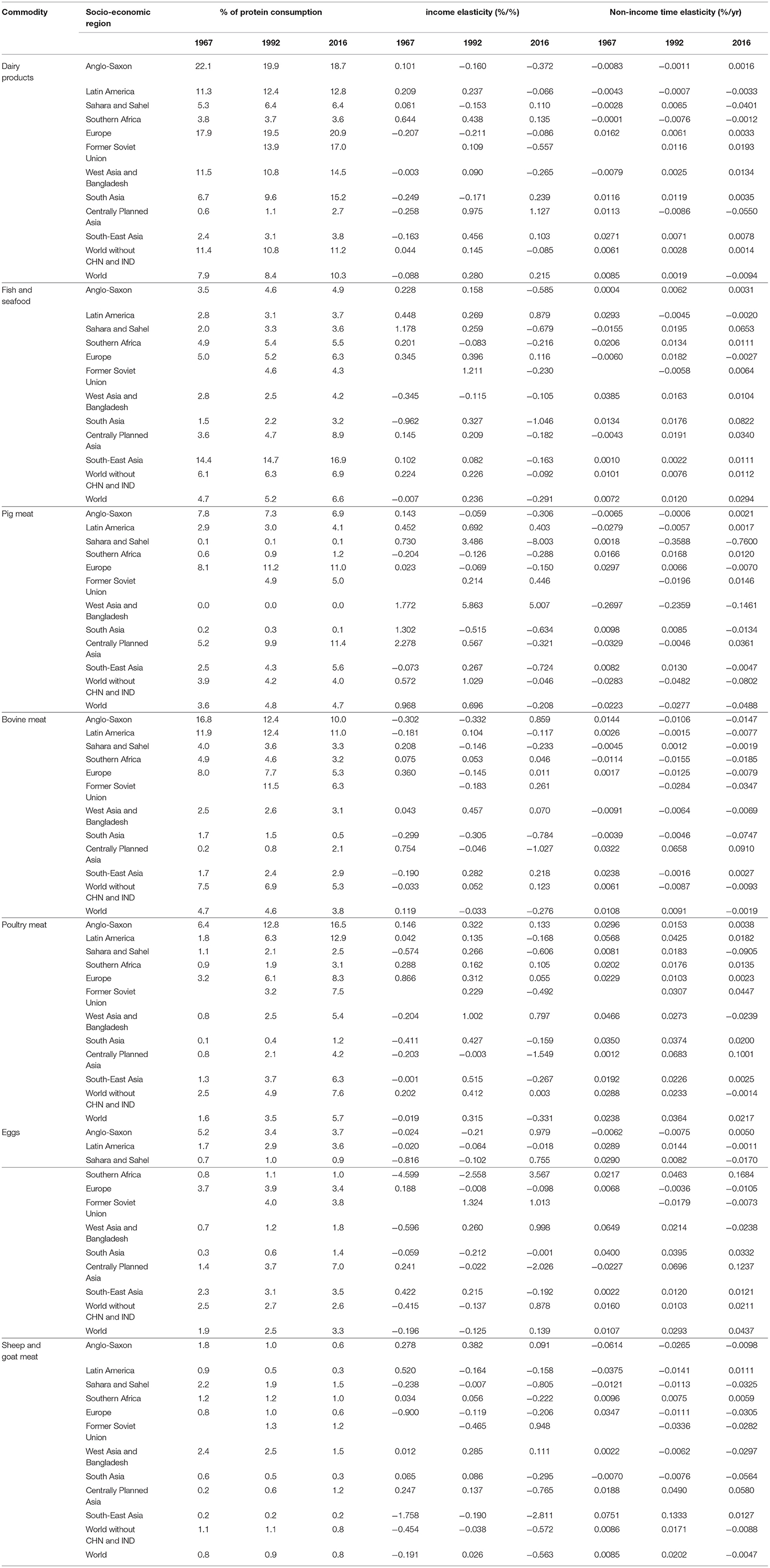
Table 3. Time trends of the contributions made to protein consumption by animal source food commodities, and of their estimated income elasticities (β) and non-income time elasticities (γ). CHN: China, IND: India.

As in sections Energy and Protein Consumption and Animal and Plant Source Food Consumption, most of the global commodity-specific patterns are dominated by CPA and South Asia with their very large human populations: on average in the rest of the world (viz. the entries “world without CHN and IND” in Table 3), only bovine meat (a reduction from 7.5 in 1967 to 5.3% in 2016) and poultry meat (an increase from 2.5 to 7.6%) show any noteworthy timetrend in their contribution to protein consumption. By contrast, CPA increased its proportional consumption of pig meat and of fish and seafood twofold; of dairy products, poultry meat and eggs more than fourfold; of sheep and goat meat sixfold; and of bovine meat tenfold. At the same time, Southern Asia reduced its proportional consumption of mammalian meat, and increased its proportional consumption of dairy products and fish and seafood twofold, of eggs fivefold, and of poultry meat twelvefold.

However, underlying this apparently stable “average of the rest of the world,” the contribution of dairy products to protein consumption increased from 12 to 15% in West Asia and decreased from 22 to 19% in the Anglo-Saxon world; for pig meat, an increase from 8 to 11% in Europe and a decrease from 8 to 7% in the Anglo-Saxon world; for poultry meat, increases from 2 to 13% in Latin America vs. from 1.1 to 2.5% in Sahara and Sahel. In summary, there are considerable regional differences in the time trends of these consumption patterns. We would then expect much variation in the income- and non-income-related driving factors, too. The development of the β and γ coefficients is most efficiently described by the estimates for pig meat, bovine meat, and eggs. The other four commodities have patterns somewhere between these three, as follows.

Pig Meat

In terms of the contribution of pig meat to protein consumption and its increase over time, Latin America shows positive β estimates and negative or close-to-zero γ estimates throughout, so the contribution increase there is clearly income-driven. The same holds for CPA for the first ¾ of the reporting period; after that, the pattern turns around. The regional β and γ estimates for Europe are both positive early on and then turn to negative; something similar happens in South-East Asia. Figure 8 shows the country-level detail behind this, with a very strong variation in the γ and particularly the β estimates across Europe, even at the high consumption levels prevalent there; the regional estimates for pig meat for Europe in Table 3 must be interpreted with caution. The regional estimates for South-East Asia are dominated by Indonesia (because of its large population) with its very low pig meat consumption levels and this creates instability of the regional estimate too.

FIGURE 8

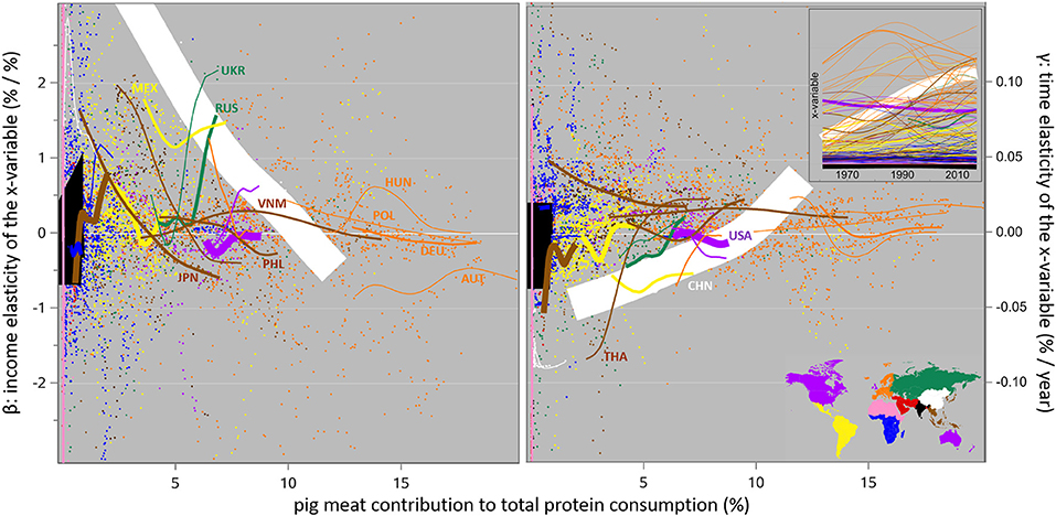
Figure 8. Regression coefficients of the logarithm of the proportions of daily protein consumption that are based on pig meat, on the logarithm of annual income (β: the income elasticity, adjusted for time-related non-income effects), and on time and its associated non-income effects (γ: the time elasticity, adjusted for income effects), from 1961 to 2017. Note that the x-axes show the actual contribution % levels, not time; the time trends of the x-variable are shown in the inset. See Figure 6 for details on the lay-out.

Bovine Meat

In terms of the contribution of bovine meat to protein consumption and its change over time, the most interesting regions are the former Soviet Union, the Anglo-Saxon world, and Latin America, where the contribution decreased over time. In the former Soviet Union, the γ estimates are negative in 1992 and 2016, so there were non-income drivers active all the time; but the β estimates change sign over time: the contribution decrease was also income-driven early on. The β and γ patterns in the Anglo-Saxon world are opposite to the ones for pig meat consumption, which also went down in that region. The γ patterns for Latin America suggest little non-income influence in either direction, but the β estimates seem confusing; again, the underlying country-level detail (Figure 9) shows much variation in the γ and particularly the β estimates across this region: the regional estimates for bovine meat for Latin America in Table 3 must be interpreted with caution. CPA and South-East Asia are interesting cases too because the bovine meat contribution increased there somewhat from extremely low initial levels. Those increases started as income-driven in CPA and changed to non-income driven at a later stage; the pattern for South-East Asia is opposite to that.

FIGURE 9

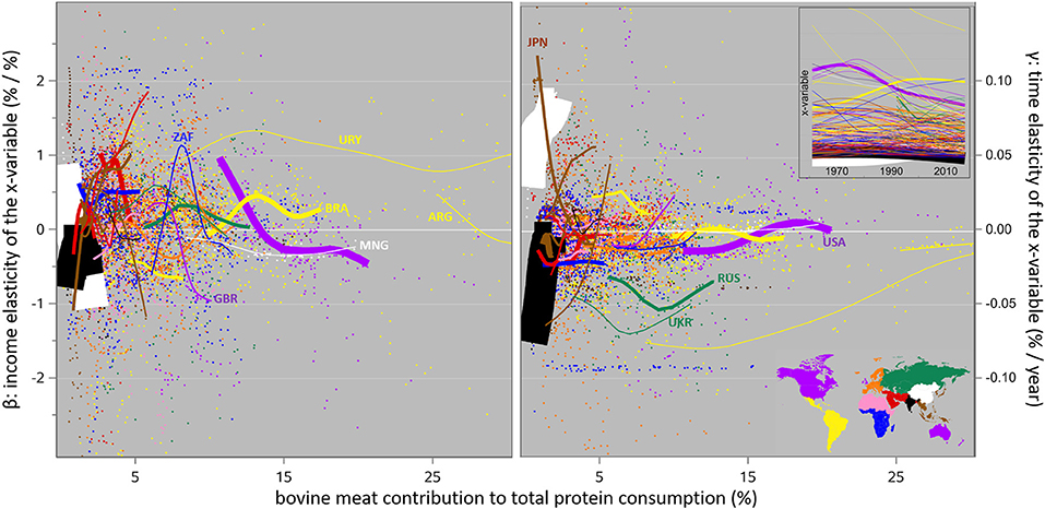
Figure 9. The same relations as in Figure 8, for bovine meat.

Eggs

In terms of the contribution of eggs to protein consumption and its change over time, the most interesting regions are South Asia and CPA where the contribution increased more than fourfold, and the Anglo-Saxon world where it decreased. The increase in South Asia is clearly non-income-driven, with negative β estimates and positive γ ones throughout. In CPA we see the now familiar pattern of a shifting income-driven to non-income-driven pattern. And the Anglo-Saxon β patterns are confusing again, likely due to considerable variation across this region as shown in Figure 10.

FIGURE 10

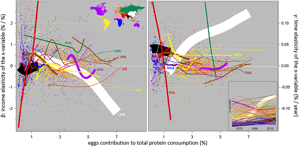
Figure 10. The same relations as in Figure 8, for eggs.

Dairy Products

In terms of the contribution of dairy products to protein consumption and its change over time, the most interesting regions are South Asia and CPA where the contribution increased more than two- and fourfold, the Anglo-Saxon world where it decreased, and Latin America and Europe where it increased by about 15% only. The increases in South Asia and CPA were clearly non-income driven initially and shifted to a strong income drive later on; the reduction in the Anglo-Saxon world shows that same pattern, with the β estimates changing from moderately negative to decidedly positive and the γ ones doing the opposite; the β and γ patterns for Latin America vs. Europe are almost opposite to each other, with considerable variation within Latin America as shown in Supplementary Figure 4.

Poultry Meat

In terms of the contribution of poultry meat to protein consumption and its change over time, the most interesting regions are West Asia and Bangladesh and Latin America where the contribution increased sevenfold, and Sahara and Sahel and the Anglo-Saxon world where it “only” more than doubled. The increase in West Asia and Bangladesh was clearly non-income driven initially and shifted to a strong income drive later on, while Latin America shows more or less the opposite pattern. The Anglo-Saxon world shows positive β and γ estimates all the time; those for Sahara and Sahel are confusing in Table 3 and better illustrated in Supplementary Figure 5 where we also see that Pakistan and Bangladesh with their large human populations and very low poultry meat consumption levels play the same confusing role as Indonesia does in section Pig Meat.

Fish and Seafood

In terms of the contribution of fish and seafood to protein consumption and its change over time, the most interesting regions are South-East Asia where the contribution is very high and slowly increasing, and CPA where it is low but more than doubled. The slow increase in South-East Asia was income-driven initially but not so later on, and the fast increase in CPA shows that same pattern even more strongly. Within South-East Asia, Supplementary Figure 6 reveals considerable variation in these patterns: there is a strong decrease of the contribution in the Philippines archipelago where fish seems to be gradually replaced by poultry and pig meat, in contrast to the nearby Indonesia archipelago where the contribution of fish consumption shows the strongest increase of all the commodities and practically all of it is not income driven. Hence again, the regional estimates for fish and seafood for South-East Asia in Table 3 must be interpreted with caution.

Sheep and Goat Meat

In terms of the contribution of sheep and goat meat to protein consumption and its change over time, the most interesting regions are Sahara and Sahel and West Asia and Bangladesh, where the contribution is highest on average (but declining like everywhere else apart from CAP with its very low levels). These two regions show completely opposite patterns in their β estimates, and similar patterns in their γ estimates. The next highest consumer is the Anglo-Saxon world; this is where the contribution of sheep and goat meat shows the largest within-region varibility in its driving factors of all the region-commodity combinations analyzed here, see Supplementary Figure 7.

A common pattern here is that the β and γ estimates are much more variable for the individual commodities of this section (Figures 8–10, Table 3, and Supplementary Figures 4–7) than for total and ASF-sourced consumption (Figures 6, 7 and Table 2), particularly at the lower consumption levels.

In summary, dairy products contribute most to worldwide protein consumption; this proportion increases mainly due to non-income-driven increases in South Asia. Fish and seafood come next with strong partly income-related increases in Africa and Asia. The strongest increase is for eggs (particularly in China, USA and Japan, see Figure 10) and poultry meat (particularly in the Americas and Europe, see Supplementary Figure 5), mainly non-income-driven. The contribution of pig meat increases slowly, mainly in China, South-East Asia and Latin America with variable income vs. non-income drivers. The contribution of bovine meat decreases, mainly in Europe and the Americas (not particularly income-related). The contribution of sheep and goat meat is stable worldwide but decreases in countries with high initial levels. Most importantly, there are considerable differences among socio-economic regions and among countries in the interplay between the income and non-income effects on the dynamics of these consumption patterns.

Discussion

In this study, food consumption and income data are analyzed with a statistical approach based on (i) Bodirsky et al. (2015) who included a “year” variable and its interaction with income in their double-logarithmic model to implicitly account for time-variant non-income factors (analyzing the consumption of energy and of its ASF-based proportion in 162 countries across 46 years) and reported a single set of global parameter estimates for each of those two response variables; (ii) Gale and Huang (2007) who applied a log-log-inverse model to allow the regression coefficient estimates (i.e., the elasticities) to change with income, analyzing the consumption of 58 commodities in a single country during 2 years with “year” included in the model as a dummy variable; and (iii) Muhammad et al. (2011) who analyzed the consumption of eight commodities recorded in 144 countries in a single year on a within-country basis. These approaches are combined here, and (iv) this is done longitudinally across the 1961–2017 period, (v) for energy, protein, and each of eight animal source food commodities (ASF as such, dairy products, eggs, fish and seafood, and bovine, sheep and goat, pig and poultry meat), with (vi) consumption quantified not in terms of financial expenditure but in terms of the contribution of a given commodity to total energy or protein consumption. As far as I am aware, these six approaches have not been combined before; most importantly, the combination of (i) and (ii) allows for the estimation of income and non-income elasticities that vary with income and over time. Further, (iii) and (iv) do this on a country-by-year level across the world, and (v) and (vi) make the exercise relevant for livestock production science and its role in human nutrition.

Data

My socio-economic regions were defined more or less arbitrarily; the same holds for earlier groupings by Lotze-Campen et al. (2008) and Femenia (2019). Obvious disputable details include the grouping together of (i) Japan, Myanmar and Papua New Guinea, (ii) Norway, Portugal and Moldova, and (iii) Kuwait, Afghanistan and Bangladesh. As always, “perfect grouping” of any complex entity is impossible. Note that the grouping plays no role in the statistical analyses as such, but only in presenting the results in Tables 2, 3 and in the Figures 1–10.

The most relevant income-related parameter for our current purposes would be the disposable income at the consumer level (household disposable income: HHDI as reported by OECD). Instead, the GDP parameter used here quantifies the total income earned in a country by households, companies and government. The difference is mainly due to taxation, depreciation, and undistributed company profit. HHDI recording is a relatively recent activity with few data available from before 1990, and the subsequent data is limited to OECD countries and under much methodological debate (e.g., Deaton, 2005); the same holds for household consumption expenditure (CPE) as reported by the World Bank. HHDI and CPE are shown in relation to GDP in Supplementary Figure 8: GDP levels around int-$ 20,000 and int-$ 40,000 overestimate HHDI by 10–70% and by 15–75%, respectively, and overestimate CPE substantially more, particularly at the lowest and highest income levels. Most importantly for our current purposes, the differences are not uniform and not linear against GDP (e.g., Birdsall and Meyer, 2014; Diacon and Maha, 2015), so there is no realistic way to convert GDP to either of these levels without considerable loss of information. It follows that the true disposable income elasticities are systematically (and unpredictably) underestimated, both in this study and in others based on GDP.

Also, the various forms of income measurement come with their own specific types and sources of error and bias. Moore et al. (2000), Milanovic (2002), Meyer et al. (2015), and Meyer and Mittag (2019) describe shortcomings of survey data like coverage or unit non-response (who is included in the data), item non-response (which details are reported) and under-reporting (people typically do not report their entire income). Meyer and Mittag (2019) discuss possible ways to overcome these issues.

A clear drawback of the type of data analyzed here is that everything is expressed on the country level—and countries vary in their population size. In populous countries such as China (1,414 million people in 2016), India (1,325 million) or USA (323 million), more or less coherent groups of about half a million people could likely be identified with extreme consumption patterns similar to what we see in Supplementary Figure 5 for Saint Lucia (0.2 million people); in Figure 7 and Supplementary Figures 6, 7 for Iceland (0.3 million); in Supplementary Figure 7 for Djibouti (0.9 million). But that kind of resolution is not possible at the macro recording level of these data; it requires more detailed studies such as the single-country micro-surveys carried out in China (Gale and Huang, 2007), India (Gandhi and Zhou, 2010; Kumar et al., 2011), Canada (Pomboza and Mbaga, 2007), or the Czech Republic (Syrovátka, 2004). Wooldridge (2010) and Baltagi (2013) describe the pros and contras, and the statistical features, of the various approaches; see also Westhoek et al. (2015, p. 24). It follows that the true variation in consumption patterns is systematically underestimated here.

The conversion factors that represent the protein and energy content of the various commodities (from Appendix I of FAO, 2001) form a crucial element behind the consumption patterns analyzed here, but are inevitably generalized across the world and over time; a more time- and location-specific dataset will be very difficult to put together as witnessed by FAO's INFOODS information at www.fao.org/infoods/infoods/tables-and-databases/en. For example, pig meat is rated too fat for the more recent years in the western world (where it is consumed most). Current dietary information sources in Germany, France, Australia and USA (tinyurl.com/y59buzxf; tinyurl.com/y4fmqnl9; tinyurl.com/y6xze5lo; tinyurl.com/ycbgr3p3) rate pig meat at 0.05 to 0.14 gram protein per kcal energy, as opposed to the FAO (2001) conversion factor of 0.04 g/kcal mentioned in connection to Figure 2 (section General Patterns of Consumption in Relation to Income). The latter value derives from data published in the 1990s and probably earlier, and the lean meat content of the typical pig carcass in the western world increased from 51% in 1985 to 63% in 2015 (updated from Figure 1 in Knap, 2014), largely due to a reduction of the fat content. As another example that works the other way around, Bijl et al. (2013) their Figure 1) show that the protein-to-fat ratio in cow milk in the Netherlands decreased from 0.9 in 1958 to 0.8 in 2010. It follows that many of the contributions to energy or protein consumption reported here may be over- or underestimated, particulary for the earlier and later years in the data.

Interpretation of the Elasticity Estimates

A striking feature of the elasticity estimates for the individual food commodities (Figures 8–10 and Table 3) is their wide variability at the lower consumption levels, in contrast to the much narrower patterns for total energy and protein consumption, and for the ASF contribution to them, as in Figures 6, 7 and Table 2. As mentioned in connection to Figure 5 (section Properties of the Elasticity Estimates), the estimates are not systematically less (or more) accurate at those lower levels, so this feature is not likely due to inappropriate data. But it does seem to be much easier to statistically unravel the income effect from the non-income ones (β vs. γ) when consumption is higher. A statistical explanation would be that the higher consumption levels allow for more variation between datapoints (i.e., between years within a country) that can be statistically exploited. Alternatively, in real life it is easier to substitute those individual commodities (e.g., shift to poultry meat when fish and seafood becomes more expensive, as has been the case in Europe the past decade) than to do this on the ASF-vs.-PSF or on the consume-vs.-not-consume level.

It is difficult to compare my results to the existing literature, for several reasons.

First, the econometric demand studies in the literature apply various types of regression model (see section Statistical Analysis), all with their statistical peculiarities. Obviously, it will be difficult to compare elasticity estimates from any two of these methods, which automatically raises the question how any food-related policy on the regulatory level should interpret them. The same holds even more for the more complex simulation models that are used to study consumption trends for long-term prediction purposes, see Femenia (2019; her Table 6), Valin et al. (2014), and Von Lampe et al. (2014). Indeed, the latter two studies are contributions to a “global economic model intercomparison activity undertaken as part of the AgMIP Project (www.agmip.org)” that “aims to substantially advance our understanding of model strengths, weaknesses, and uncertainty while also developing new approaches including data integration and transdisciplinary modeling frameworks.” Von Lampe et al. (2014) recommend studies “that would allow for the generation of comparable price elasticity matrices for area, yield, and final demand across agricultural products.”

Second, published elasticity estimates are very variable in magnitude. For example, Femenia (2019) performed a meta-analysis of income elasticity estimates published worldwide between 1973 and 2014. Her estimates for consumption of meat and fish or dairy products can be divided into two groups based on socio-economic region: in the Americas, the EU, and East and South Asia (i.e., 76% of the 2016 world population), both commodities show mean income elasticities ranging from +0.5 to +0.8 with very large standard deviations ranging from 0.5 to 0.8. In the rest of the world, the mean income elasticities show that same range but the standard deviations are much smaller (0.1–0.4). It follows that three quarters of the world population lives in countries where these income elasticities either (i) really vary from decidedly negative to very strongly positive or (ii) are extremely difficult to estimate accurately; for the rest of the world, dominated by low-income countries, these estimates seem to be more consistently positive.

Third, the aggregation level of the studied commodities (e.g., ASF > meat and fish > meat > bovine meat > hamburger) can strongly influence the results. Hassan and Johnson (1977) estimated income elasticities of consumption of a wide variety of food commodities in Canada. The estimates (from their Table 8) range from −0.2 to +0.2 for seven types of pig meat, from −0.2 to +0.5 for seven types of bovine meat, from −0.6 to +0.4 for five types of fish, and from −0.6 to +0.7 for ten types of dairy product. Likewise, Gandhi and Zhou (2010; their Tables 8, 9) report income elasticities ranging from −0.1 to +2.2 for five types of dairy product consumed in India. It follows that income elasticities for aggregated commodities such as “dairy products” or “fish and seafood,” estimated on a country basis, depend considerably on the range of such commodities included in the aggregate.

Fourth, “consumption” can be quantified in multiple ways. The economic literature measures per caput consumption either as a quantity (e.g., kg per year) or, more often, in terms of financial expenditure (e.g., $ per year). The biophysical approach to measure consumption in terms of the contribution to total energy or protein consumption is very different from that. Muhammad et al. (2011) analyzed a cross-section dataset of consumption in 146 countries in 2005, regressing the budget share of each commodity (i.e., the proportion of total financial expenditure spent on purchasing it) on income, price (if the purchased volume does not change, a higher price will increase the budget share), and substitution effects (if other commodities are bought instead, a higher price will reduce it). Their income elasticity estimates for dairy products and fish can be compared to my corresponding β estimates for 2005, bearing in mind that the two compared models (i) are different in structure and (ii) relate different entities to income, i.e., the proportion of total financial expenditure, vs. the proportion of total protein consumption.

This comparison shows that Muhammad's and my elasticity estimates are essentially uncorrelated (r = +0.2 for dairy products, r = −0.1 for fish), and the actual consumption levels do not play any role in the relationships. Moreover, Muhammad's expenditure-related elasticities show strongly significant (P < 0.0001) differences between the various socio-economic regions with the lowest estimates in Europe and the Anglo-Saxon world, and the highest ones in Africa; this pattern is completely absent (P > 0.9) among my protein-consumption-related elasticities.

Income and Non-income Effects

Bodirsky et al. (2015) concluded that income, time and their interaction are “significant predictors for” the ASF contribution to energy consumption; the interaction term was particularly influential at the higher income levels. Gale and Huang (2007) fitted the year effect as a dummy variable for their 2002–2003 data, and found it to be “significant in about half of the equations.” Likewise, Milford et al. (2019) report significant effects of time-variant factors such as urbanization, globalization and population density on the global consumption of (ruminant) meat. They notice that “previous econometric assessments […] often considered a much smaller number of explanatory variables, usually prices and income. Thereby, they may have overestimated the effect of income on meat demand, as other explanatory variables such as urbanization or female participation are strongly correlated with income. […] Food demand models using just income and price elasticities should be applied with care.”

The strong significance of the non-income γ coefficients from my analysis is therefore not surprising. Rather, the novel elements as illustrated in Figures 8–10 and Supplementary Figures 4–7 are (i) the considerable variation of the β and γ estimates between countries within each socio-economic region, (ii) their equally considerable changes over time within countries, often moving from positive to negative or vice versa, and (iii) the variable association patterns between β and γ at both these levels.

Extensions and Applications

We have here a very rich dataset on consumption of ten food commodities across 50 years in 150 countries with two driving factors to be explored. Its analysis shows substantial variation in all the estimated parameters over time and across the world, as illustrated in Figures 8–10 and Supplementary Figures 4–7. This variation is the most striking element of my findings; it also features very clearly in Figures 1, 3 of Bodirsky et al. (2015), but that study focuses on aggregated global patterns and therefore ignores the variation, with good reason. Most other studies do not mention it at all, or treat it as a nuisance factor, or do not try to quantify it in the first place. Some of this variation is likely the consequence of specific events that happened over the 1961–2017 period studied here, such as the OPEC-triggered oil shocks of the 1970s, the Latin American debt crisis of 1980s, the European CAP reform of the 1990s, the wordwide recession of the late 2000s, or the financial crises in Russia and China of the mid-2010s, and in another dimension the epidemics of H3N2 influenza in the late 1960s, SARS from China in the early 2000s, HIV in Africa from the 2000s, or H1N1 influenza from the Americas and Ebola in West-Africa in the early 2010s. It would also be interesting to group the β and γ estimates in terms of some quantiles of GDP, or of poultry meat or fish consumption (or wheat or rice consumption), or of the various non-income factors of statistical model (2). But this is beyond the scope of this article: a topic for further analysis.

Elasticity-of-consumption estimates play important roles in forecasting long-term consumption patterns and their associated production requirements—with food security, land use, water use and climate change as typical focal points, and with worldwide policymakers as the intended audience; e.g., Bodirsky et al. (2015), Gouel and Guimbard (2019), and Warren et al. (2021). The International Institute for Applied Systems Analysis (IIASA, tntcat.iiasa.ac.at/SspDb) predicts population size, GDP and urbanization rate of many countries up to the year 2100. These predictions follow five scenarios introduced as Shared Socioeconomic Pathways (SSPs) by O'Neill et al. (2014), defined in terms of technological, economical and political factors that influence (i) mitigation of climate change and (ii) the capability of coping with it. Across these SSPs, IIASA predictions for the year 2100 range from 6.9 to 12.6 billion people for the world population, from 22 to 138 k 2005-USD for worldwide per caput GDP, and from 58 to 93% for the worldwide urbanization rate. The consumption levels of any commodity can then be forecasted from the predicted GDP and the relevant estimate for the income elasticity of consumption, and likewise for other factors such as urbanization rate. One of the key attributes of such consumption projections is their intrinsic accuracy level, which will depend on (i) accuracy of elasticity estimates as illustrated in Figure 5, and (ii) variability of the predicted independent variables (such as GDP) across the five SSPs.

With country-specific elasticity estimates such as mine, that approach would allow for forecasting the consumption of (or rather, the demand for) the various ASF commodities on a per-country basis. The main challenge of such a study will be to find a sensible way to extrapolate the time trends of the elasticity estimates into the future.

Conclusions

Patterns of animal source food (ASF) consumption differed between various parts of the world, and they changed over time. These differences and changes were significantly related to income, but considerably more related to time-dependent non-income factors.

Within-country income elasticity estimates of total energy and protein consumption between 1961 and 2017 ranged from −1 to +1: when income increased by 1%, consumption changed by −1 to +1%. The corresponding non-income time elasticity estimates ranged from −0.05 to +0.05% per year: every year, adjusted for income, consumption changed by −0.05 to +0.05%. The elasticity estimates for the contribution to energy and protein consumption of animal-source food ranged twice as wide as these. Those for the contribution to protein consumption of dairy products, fish and seafood, poultry meat, pig meat, bovine meat, eggs, and sheep and goat meat ranged at least three times as wide.

Both the income and the non-income elasticity estimates for the contributions of those commodities to protein consumption changed considerably over time in many countries; their association to each other was very variable too, both between and within countries.

Much of all this variation took place at the lower consumption levels, possibly because the higher ones provided more within-country variation over time that can be exploited statistically. Alternatively, in real life it is easier to substitute those individual commodities than to do this on the ASF-vs.-PSF or on the consume-vs.-not-consume level.

Considering all this, any attempt to forecast the consumption of animal source food (and particularly of its individual commodities) on a more detailed level than globally and on a longer term than a decade should should include an income-independent time factor and be very careful with regard to the elasticity coefficients used.

Data Availability Statement

The original contributions presented in the study are included in the article/Supplementary Material, further inquiries can be directed to the corresponding author.

Author Contributions

The author confirms being the sole contributor of this work and has approved it for publication.

Conflict of Interest

PK is employed by Genus PIC. This study received funding from Genus PIC. The funder was not involved in the study design, collection, analysis, interpretation of data, the writing of this article or the decision to submit it for publication.

Publisher's Note

All claims expressed in this article are solely those of the authors and do not necessarily represent those of their affiliated organizations, or those of the publisher, the editors and the reviewers. Any product that may be evaluated in this article, or claim that may be made by its manufacturer, is not guaranteed or endorsed by the publisher.

Acknowledgments

The world map of the insets in many of the Figures is courtesy of www.mapchart.net.

Supplementary Material

The Supplementary Material for this article can be found online at: https://www.frontiersin.org/articles/10.3389/fsufs.2021.732915/full#supplementary-material

References

Alexander, D. L. J., Tropsha, A., and Winkler, D. A. (2015). Beware of R²: simple, unambiguous assessment of the prediction accuracy of QSAR and QSPR models. J. Chem. Inf. Model. 55, 1316–1322. doi: 10.1021/acs.jcim.5b00206

PubMed Abstract | CrossRef Full Text | Google Scholar

Alexander, P., Brown, C., Arneth, A., Finnigan, J., Moran, D., and Rounsevell, M. D. A. (2017). Losses, inefficiencies and waste in the global food system. Agric. Syst. 153, 190–200. doi: 10.1016/j.agsy.2017.01.014

PubMed Abstract | CrossRef Full Text | Google Scholar

Baltagi, B. H.. (2013). Econometric Analysis of Panel Data, 5th Edn. Chichester, UK: Wiley.

Google Scholar

Bennett, M. K.. (1941). International contrasts in food consumption. Geogr. Rev. 31, 365–376. doi: 10.2307/210172

CrossRef Full Text | Google Scholar

Bijl, E., Van Valenberg, H. J. F., Huppertz, T., and Van Hooijdonk, A. C. M. (2013). Protein, casein, and micellar salts in milk: current content and historical perspectives. J. Dairy Sci. 96, 5455–5464. doi: 10.3168/jds.2012-6497

PubMed Abstract | CrossRef Full Text | Google Scholar

Birdsall, N., and Meyer, C. J. (2014). The Median Is the Message: A Good-Enough Measure of Material Well-Being and Shared Development Progress. CGD Working Paper 351. Washington DC: Center for Global Development. Available online at: www.cgdev.org/publication/median-message-good-enough-measure-material-wellbeing-and-shared-development-progress.

Google Scholar

Blommaert, A., Hens, N., and Beutels, P. (2014). Data mining for longitudinal data under multicollinearity and time dependence using penalized generalized estimating equations. Comput. Stat. Data Anal. 71, 667–680. doi: 10.1016/j.csda.2013.02.023

CrossRef Full Text | Google Scholar

Bodirsky, B. L., Rolinski, S., Biewald, A., Weindl, I., Popp, A., and Lotze-Campen, H. (2015). Global food demand scenarios for the 21st Century. PLoS ONE 10:e0139201. doi: 10.1371/journal.pone.0139201

PubMed Abstract | CrossRef Full Text | Google Scholar

Bolt, J., Inklaar, R., Jong, D. E., and Van Zanden, H. (2018). Rebasing 'Maddison': New Income Comparisons and the Shape of Long-Run Economic Development. Maddison Project Working Paper 10, GGDC Research Memorandum 174, University of Groningen. Available online at: www.rug.nl/ggdc/html_publications/memorandum/gd174.pdf

Google Scholar

Burnham, K. P., and Anderson, D. R. (2004). Multimodel inference: understanding AIC and BIC in model selection. Soc. Methods Res. 33, 261–304. doi: 10.1177/0049124104268644

CrossRef Full Text | Google Scholar

Capper, J. L.. (2020). Opportunities and challenges in animal protein industry sustainability: the battle between science and consumer perception. Anim. Front. 10, 7–13. doi: 10.1093/af/vfaa034

PubMed Abstract | CrossRef Full Text | Google Scholar

Deaton, A.. (2005). Measuring poverty in a growing world (or measuring growth in a poor world). Rev. Econ. Stat. 87, 1–19. doi: 10.1162/0034653053327612

CrossRef Full Text | Google Scholar

Diacon, P. E., and Maha, L. G. (2015). The relationship between income, consumption and GDP: a time series, cross-country analysis. Procedia Econ. Finance 23, 1535–1543. doi: 10.1016/S2212-5671(15)00374-3

CrossRef Full Text | Google Scholar

Dolislager, M. J.. (2017). Food consumption patterns in light of rising incomes, urbanization and food retail modernization: evidence from Eastern and Southern Africa (Ph.D. thesis). Michigan State University, East Lansing MI.

Google Scholar

Efron, B., and Tibshirani, R. (1986). Bootstrap methods for standard errors, confidence intervals, and other measures of statistical accuracy. Stat. Sci. 1, 54–75. doi: 10.1214/ss/1177013815

CrossRef Full Text | Google Scholar

Engel, E.. (1857). Die vorherrschenden Gewerbszweige in den Gerichtsämtern mit Beziehung auf die Productions- und Consumtionsverhältnisse des Königreichs Sachsen. Zeitschrift des statistischen Bureaus des Königlich Sächsischen Ministerium des Inneren 8-9, 28–29. Available online at: https://www.econstor.eu/bitstream/10419/233572/1/wista-2021-2-126-136.pdf

Google Scholar

FAO (2001). Food Balance Sheets: A Handbook. Rome: Food and Agriculture Organization. Available online at: www.fao.org/economic/the-statistics-division-ess/publications-studies/publications/nutritive-factors/en

Google Scholar

FAO (2004). Human Energy Requirements. FAO Food and Nutrition Technical Report Series 1, Rome: Food and Agriculture Organization. Available online at: www.fao.org/3/y5686e/y5686e00.htm

Google Scholar

FAO (2009). The state of Food and Agriculture: Livestock in the Balance. Rome: Food and Agriculture Organization. Available online at: http://www.fao.org/3/i0680e/i0680e.pdf

Google Scholar

Fekedulegn, B. D., Colbert, J. J., Hicks, R. R., and Schuckers, M. E. (2002). Coping With Multicollinearity: An Example on Application of Principal Components Regression in Dendroecology. Research Paper NE-721, Washington DC: United States Department of Agriculture. Available online at: www.fs.fed.us/ne/newtown_square/publications/research_papers/pdfs/2002/rpne721.pdf.

Google Scholar

Femenia, F.. (2019). A meta-analysis of the price and income elasticities of food demand. German J. Agric. Econ. 68, 77–98. Available online at: www.gjae-online.de/articles/a-meta-analysis-of-the-price-and-income-elasticities-of-food-demand

PubMed Abstract | Google Scholar

Fernandez, G.. (2007). “Model selection in PROC MIXED: a user-friendly SAS^® macro application,” in SAS Global Forum 2007 Proceedings, Paper 191-2007. Available online at: www2.sas.com/proceedings/forum2007/191-2007.pdf

Google Scholar

Gale, F., and Huang, K. (2007). Demand for Food Quantity and Quality in China. Economic Research Report 32, Washington DC: United States Department of Agriculture. Available online at: papers.ssrn.com/sol3/papers.cfm?abstract_id=1739091

Google Scholar

Gandhi, V. P., and Zhou, Z. Y. (2010). Rising demand for livestock products in India: nature, patterns and implications. Aust. Agribus. Rev. 18, 103–135. Available online at: ageconsearch.umn.edu/bitstream/114421/2/Vasant_Zhang-Yue.pdf

Google Scholar

Goreux, L. M.. (1960). Income and food consumption. Mon. Bull. Agric. Econ. Stat. 9, 1–13.

Google Scholar

Gouel, C., and Guimbard, H. (2019). Nutrition transition and the structure of global food demand. Am. J. Agric. Econ. 101, 383–403. doi: 10.1093/ajae/aay030

CrossRef Full Text | Google Scholar

Guo, A. L.. (2000). Structural change in the impact of income on food consumption in China 1989-1993. Econ. Dev. Cult. Change 48, 737–760. doi: 10.1086/452475

CrossRef Full Text | Google Scholar

Gustavsson, J., Cederberg, C., Sonesson, U., Van Otterdijk, R., and Meybeck, A. (2011). Global Food Losses and Food Waste: Extent, Causes and Prevention. Rome: Food and Agriculture Organization. Available online at: www.fao.org/3/a-i2697e.pdf

Google Scholar

Hassan, Z. A., and Johnson, S. R. (1977). Urban Food Consumption Patterns in CANADA. Publication 77/1, Ottawa, ON: Information Division, Agriculture Canada. Available online at: ageconsearch.umn.edu/record/149019.

Google Scholar

Houthakker, H. S.. (1957). An international comparison of household expenditure patterns, commemorating the centenary of Engel's law. Econometrica 25, 532–551. doi: 10.2307/1905382

CrossRef Full Text | Google Scholar

Huang, Q., and Zhu, L. (2015). “The %IC_MIXED: A SAS^® macro to produce sorted information criteria list for PROC MIXED for model selection,” in SAS Global Forum 2015 Proceedings, Paper 3504-2015. Available online at: support.sas.com/resources/papers/proceedings15/3504-2015.pdf

Google Scholar

Juréen, L.. (1956). Long-term trends in food consumption: a multi-country study. Econometrica 24, 1–21. doi: 10.2307/1905255

CrossRef Full Text | Google Scholar

Kearney, J.. (2010). Food consumption trends and drivers. Philos. Trans. R. Soc. B 365, 2793–2807. doi: 10.1098/rstb.2010.0149

PubMed Abstract | CrossRef Full Text | Google Scholar

Keyzer, M. A., Merbis, M. D., Pavel, I. F. P. W., and Van Wesenbeeck, C. F. A. (2005). Diet shifts towards meat and the effects on cereal use: can we feed the animals in 2030? Ecol. Econ. 55, 187–202. doi: 10.1016/j.ecolecon.2004.12.002

CrossRef Full Text | Google Scholar

Knap, P. W.. (2013). “Pig breeding for increased sustainability,” in Sustainable Food Production, eds P. Christou, R. Savin, B. A. Costa-Pierce, I. Misztal, and C. B. A. Whitelaw (New York NY: Springer Science+Business Media), 1256–1295.

Google Scholar

Knap, P. W.. (2014). “Pig breeding goals in competitive markets,” in Proceedings of the 10th World Congress of Genetics Applied to Livestock Production (Vancouver, BC). Available online at: wcgalp.org/system/files/proceedings/2014/pig-breeding-goals-competitive-markets.pdf

Google Scholar

Kumar, P., Kumar, A., Parappurathu, S., and Raju, S. S. (2011). Estimation of demand elasticity for food commodities in India. Agric. Econ. Res. Rev. 24, 1–14.

Google Scholar

Kvalseth, T. O.. (1985). Cautionary note about R². Am. Stat. 39, 279–285. doi: 10.1080/00031305.1985.10479448

PubMed Abstract | CrossRef Full Text | Google Scholar

Le, T. H., Disegna, M., and Lloyd, T. (2020). National food consumption patterns: converging trends and the implications for health. Euro Choices. doi: 10.1111/1746-692X.12272

CrossRef Full Text | Google Scholar

Lopez Barrera, E., and Hertel, T. (2020). Global food waste across the income spectrum: implications for food prices, production and resource use. Food Policy 98:101874. doi: 10.1016/j.foodpol.2020.101874

CrossRef Full Text | Google Scholar

Lotze-Campen, H., Müller, C., Bondeau, A., Rost, S., Popp, A., and Lucht, W. (2008). Global food demand, productivity growth, and the scarcity of land and water resources: a spatially explicit mathematical programming approach. Agric. Econ. 39, 325–338. doi: 10.1111/j.1574-0862.2008.00336.x

CrossRef Full Text | Google Scholar

Masterman, C. J., and Viscusi, W. K. (2018). The income elasticity of global values of a statistical life: stated preference evidence. J. Benefit Cost Anal. 9, 407–434. doi: 10.1017/bca.2018.20

PubMed Abstract | CrossRef Full Text | Google Scholar

McNamee, R.. (2005). Regression modelling and other methods to control confounding. Occup. Environ. Med. 62, 500–506. doi: 10.1136/oem.2002.001115

PubMed Abstract | CrossRef Full Text | Google Scholar

Meyer, B. D., and Mittag, N. (2019). Combining Administrative and Survey Data to Improve Income Measurement. IZA Discussion Paper 12266, Bonn: IZA Institute of Labor Economics. Available online at: hdl.handle.net/10419/196764 doi: 10.3386/w25738

CrossRef Full Text | Google Scholar

Meyer, B. D., Mok, W. K. C., and Sullivan, J. X. (2015). Household surveys in crisis. J. Econ. Perspect. 29, 199–226. doi: 10.1257/jep.29.4.199

CrossRef Full Text | Google Scholar

Milanovic, B.. (2002). True world income distribution, 1988 and 1993: first calculation based on household surveys alone. Econ. J. 112, 51–92. doi: 10.1111/1468-0297.0j673

CrossRef Full Text | Google Scholar

Milford, A. B., Le Mouël, C., Bodirsky, B. L., and Rolinski, S. (2019). Drivers of meat consumption. Appetite 141, 104313. doi: 10.1016/j.appet.2019.06.005

PubMed Abstract | CrossRef Full Text | Google Scholar

Moore, J. C., Stinson, L. L., and Welniak, E. J. (2000). Income measurement error in surveys: a review. J. Off. Stat. 16, 331–361. Available online at: www.scb.se/contentassets/ff271eeeca694f47ae99b942de61df83/income-measurement-error-in-surveys-a-review.pdf

Google Scholar

Muhammad, A., Seale, J. L., Meade, B. G. S., and Regmi, A. (2011). International Evidence on Food Consumption Patterns: An Update Using 2005 International Comparison Program Data. Technical Bulletin 1929, ERS, Washington DC: United States Department of Agriculture.

Google Scholar

Neeteson-Van Nieuwenhoven, A. M., Knap, P. W., and Avendaño, S. (2013). The role of sustainable commercial pig and poultry breeding for food security. Anim. Front. 3, 52–57. doi: 10.2527/af.2013-0008

CrossRef Full Text | Google Scholar

Ng, M., Fleming, T., Robinson, M., Thomson, B., Graetz, N., and Margono, C. (2014). Global, regional, and national prevalence of overweight and obesity in children and adults during 1980–2013: a systematic analysis for the Global Burden of Disease Study 2013. Lancet 384, 766–781. doi: 10.1016/S0140-6736(14)60460-8

PubMed Abstract | CrossRef Full Text | Google Scholar

O'Neill, B. C., Kriegler, E., Riahi, K., Ebi, K. L., Hallegatte, S., Carter, T. R., et al. (2014). A new scenario framework for climate change research: the concept of shared socioeconomic pathways. Clim. Change 122, 387–400. doi: 10.1007/s10584-013-0905-2

CrossRef Full Text | Google Scholar

OSISA (2009). Strengthening Popular Participation in the African Union. Open Society Initiative for Southern Africa, Rosebank, South Africa. Available online at: www.afrimap.org/english/images/report/AfriMAP-AU-Guide-EN.pdf

Google Scholar

Pomboza, R., and Mbaga, M. (2007). The estimation of food demand elasticities in Canada. Publication 06-071-RB, Ottawa, ON: Agriculture and Agri-Food Canada. Available online at: ageconsearch.umn.edu/record/52705/files/estimation_e.pdf

Google Scholar

Popkin, B.. (1993). Nutritional patterns and transitions. Popul. Dev. Rev. 19, 138–157. doi: 10.2307/2938388

CrossRef Full Text | Google Scholar

Popkin, B. M.. (1995). Nutrition transition and the global diabetes epidemic. Curr. Diab. Rep. 15, 64. doi: 10.1007/s11892-015-0631-4

PubMed Abstract | CrossRef Full Text | Google Scholar

Regmi, A., Deepak, M. S., Seale, J. L., and Jason Bernstein, J. (2001). “Cross-country analysis of food consumption patterns,” in Changing Stucture of Global Food Consumption and Trade, ed A. Regmi, Agriculture and Trade Report WRS-01-1, ERS-MTED (Washington DC: United States Department of Agriculture), 14–22.

Google Scholar

Ritchie, H., and Roser, M. (2017). Meat and Dairy Production. Available online at: ourworldindata.org/meat-production

Google Scholar

Robinson, T. P., and Pozzi, F. (2011). Mapping Supply and Demand for Animal Source Foods to 2030. Animal Production and Health working paper 2, Rome: Food and Agriculture Organization. Available online at: http://www.fao.org/3/i2425e/i2425e.pdf

Google Scholar

SAS Institute (2018). SAS/STAT^® 15, 1. User's Guide. Cary NC: SAS InstituteInc.

Google Scholar

Seale, J., Regmi, A., and Bernstein, J. (2003). International Evidence on Food Consumption Patterns. Technical Bulletin 1904, Economic Research Service, USDA, Washington DC. Available online at: www.ers.usda.gov/webdocs/publications/47429/14755_tb1904_1_.pdf

Google Scholar

Shyma, J.. (2016). Economic growth, poverty and malnutrition in India. Ekonomik Yaklaşim 27, 165–202. doi: 10.5455/ey.35902

CrossRef Full Text | Google Scholar

Stone, R.. (1954). The Measurement of Consumers' Expenditure and Behaviour in the United Kingdom, 1920-1938, Vol. 1. Cambridge, UK: Cambridge University Press.

Google Scholar

Syrovátka, P.. (2004). Income elasticity of food expenditures of the average Czech household. Agric. Econ. 50, 309–316. doi: 10.17221/5208-AGRICECON

CrossRef Full Text | Google Scholar

Theil, H.. (1961). Economic Forecasts and Policy. Amsterdam: North-Holland.

Google Scholar

Timmer, C. P., Falcon, W. P., and Pearson, S. R. (1983). Food Policy Analysis. Baltimore MD: Johns Hopkins University Press.

Google Scholar

UN (2019). World Population Prospects 2019, Revision 1. Population Division, DESA, New York, NY: United Nations. Available online at: https://population.un.org/wpp/Download/Files/1Indicators%20(Standard)/EXCEL_FILES/1_Population/WPP2019_POP_F01_1_TOTAL_POPULATION_BOTH_SEXES.xlsx

Google Scholar

Valin, H., Sands, R. D., Van der Mensbrugghe, D., Nelson, G. C., Ahammad, H., Blanc, E. Mason d'Croz, D., et al. (2014). The future of food demand: understanding differences in global economic models. Agric. Econ. 45, 1–17. doi: 10.1111/agec.12089

CrossRef Full Text | Google Scholar

Von Lampe, M., Willenbockel, D., Ahammad, H., Blanc, E., Cai, Y., Calvin, K. Mason d'Croz, D., et al. (2014). Why do global long-term scenarios for agriculture differ? An overview of the AgMIP Global Economic Model Intercomparison. Agric. Econ. 45, 1–18. doi: 10.1111/agec.12086

CrossRef Full Text | Google Scholar

Wagenmakers, E. J., and Farrell, S. (2004). AIC model selection using Akaike weights. Psychonomic Bull. Rev. 11, 192–196. doi: 10.3758/BF03206482

PubMed Abstract | CrossRef Full Text | Google Scholar

Walpole, S. C., Prieto-Merino, D., Edwards, P., Cleland, J., Stevens, G., and Roberts, I. (2012). The weight of nations: an estimation of adult human biomass. BMC Public Health 12:439. doi: 10.1186/1471-2458-12-439

PubMed Abstract | CrossRef Full Text | Google Scholar

Warren, F., Arneth, A., Henry, R., Maire, J., Rabin, S., Rounsevell, M., et al. (2021). “Policies for food system resilience: modelling global shocks to the UK food system,” in Nature Food Submitted. Agricultural Economics Society Conference 2021. Available online at: ageconsearch.umn.edu/record/312056/files/Frances_Warren_FWarren - UK shocks paper - full draft for AES.pdf

Google Scholar

Westhoek, H., Lesschen, J. P., Leip, A., Rood, T., Wagner, S., Marco, D., et al. (2015). Nitrogen on the Table: The Influence of Food Choices on Nitrogen Emissions and the European Environment. Edinburgh: European Nitrogen Assessment Special Report on Nitrogen and Food; Centre for Ecology and Hydrology. Available online at: www.clrtap-tfrn.org/N-on-the-table

Google Scholar

Wooldridge, J. M.. (2010). Econometric Analysis of Cross Section and Panel Data. Cambridge MA: MIT Press.

Google Scholar

Wu, G.. (2016). Dietary protein intake and human health. Food Funct. 7, 1251–1265. doi: 10.1039/C5FO01530H

PubMed Abstract | CrossRef Full Text | Google Scholar