Optimizing Nutrient Recycling From Excreta in Sweden and Pakistan: Higher Spatial Resolution Makes Transportation More Attractive

Recycling essential plant nutrients like nitrogen (N), phosphorus (P), and potassium (K) from organic waste such as human and animal excreta will be an essential part of sustainable food systems and a circular economy. However, transportation is often cited as a major barrier to increased recycling as organic waste is heavy and bulky, and distances between areas of abundant waste may be far from areas with a need for fertilizers. We investigated the effect of increased input data spatial resolution to an optimization model on the weight, distance, and spatial patterns of transport. The model was run in Sweden and in Pakistan to examine cost-effectiveness of transporting excess excreta to areas of crop need after local recycling. Increasing the resolution of input data from political boundaries (municipalities and districts) to 0.083 decimal grids increased the amount of N requiring transport by 12% in Pakistan and increased P requiring transport by 14% in Sweden. The average distance decreased by 67% (to 44 km) in Pakistan but increased by 1 km in Sweden. Further increasing the resolution to 5 km grids in Sweden decreased the average transportation distance by 9 km (down to 123 km). In both countries, increasing resolution also decreased the number of long-distance heavy transports, and as such costs did not increase as much as total distance and weight transported. Ultimately, transportation in Pakistan seemed financially beneficial: the cost of transport only represented 13% of the NPK fertilizer value transported, and total recycling could even cover 78% of additional fertilizer purchases required. In Sweden, the cost of transporting excreta did not seem cost effective without valuing other potential benefits of increased recycling: costs were three times higher than the fertilizer value transported in excreta at the 5 km resolution. In summary, increasing input data resolution created a more realistic picture of recycling needs. This also highlighted more favorable cost to fertilizer value ratios which could make it easier to move forward with industry and government partners to facilitate productive recycling. Our analysis shows that in both countries increased recycling can result in better spatial nutrient balances.

Introduction

Major transformations in our global and local food systems are required to meet the UNs Sustainable Development Goals related to food security and water quality, including the need to increase the safe recycling of organic wastes such as animal and human excreta (referred to together as excreta from here on) back to agricultural areas that require these inputs (Jurgilevich et al., 2016; Trimmer et al., 2017). One of the main reasons for requiring the recovery and reuse of organic waste is related to their relatively high concentration of essential nutrients such as nitrogen (N), phosphorus (P), and potassium (K). Society faces challenges with the affordable and stable availability of these fertilizers (N and P more acutely) to all farmers, especially in developing countries, but with global significance from a long-term perspective (Vitousek et al., 2009; Jones et al., 2013; Cordell et al., 2015). At the same time, all regions of the world are also faced with water pollution associated with the loss of N and P from poor waste management [i.e., eutrophication (Smith, 2003) and associated algal toxicity and hypoxia Diaz, 2001; Hamilton et al., 2016]. Principles of circular economy (although not synonymous with sustainability Geissdoerfer et al., 2017) can be helpful in guiding the types of transformations needed in our organic waste management system (e.g., for P Vollaro et al., 2017), and circular economy has even been explicitly taken up as a framework by the European Union (EC, 2016). Still, large-scale adoption of circular economy principles and effective organic waste recycling (i.e., safe application at the right time, in the right amount, and the right place) has yet to become a reality (Ghisellini et al., 2016).

Transportation costs and logistics are often cited as major barriers to increasing the recycling needed to achieve such a circular economy. This is particularly true with excreta as it is bulky and heavy (high water content), and areas of waste production (cities and concentrated livestock) are increasingly far from areas of crop production because of land use specialization, and the nutrient to mass ratio is thus often unfavorable (Westerman and Bicudo, 2005; Keplinger and Hauck, 2006; Nicholson et al., 2012). The distance at which it is economically viable to transport excreta to agricultural crop land depends on a myriad of local factors, including the dry matter content of the excreta product, laws on treatment and application, the price of alternative nutrient sources and energy/fuel, as well as infrastructure and farming bio geophysical conditions (Flotats et al., 2009; Sharpley et al., 2016; Bloem et al., 2017). As such, reported acceptable distances vary greatly within the literature. For example, maximum hauling distances have been estimated at 50 to 100 km for swine manure in Ireland (Fealy and Schröder, 2008) compared to 40 km in the USA (Keplinger and Hauck, 2006). For beef, estimates vary from 15 to 18 km for feedlots in Canada (Freeze and Sommerfeldt, 1985), similarly 12 km for cattle from an energy perspective (Pimentel and Pimentel, 2008), but as little as 15–30 km (Paudel et al., 2009) to as much as 60 km for dairy production (Keplinger and Hauck, 2006) in the USA. Poultry manure, which is less dilute and bulky, may be transported 400 km in the USA (Sharpley et al., 2016). In Brazil, manure is usually used within a 15 km radius from where it is produced (Shigaki et al., 2006). For human excreta, which may be in the form of sludge or biosolids after treatment in a wastewater treatment plant, acceptable transport distances can vary from 0 (i.e., no recycling) to cross-country travel to find a suitable recipient (e.g., 2,000 km from Boston to Florida in the USA Bergendahl et al., 2018); but transportation is only one of the many factors that drive or inhibit recycling, including potential contaminants and social acceptance (Englande and Reimers, 2001; Metson et al., 2018; Wadsworth et al., 2018). Although the ensemble of these distance ranges is broad, for the most part the distances are shorter than what would be required to ensure total recycling within a country (e.g., Metson et al., 2016; Akram et al., 2018; Akram et al., in press). Finding ways to minimize transportation distances will thus be a critical part of moving toward a more circular organic waste economy regardless of location.

One way to inform decision making to minimize transportation distances is through optimization modeling, however the nature of the data inputs will affect the results. The quality, and spatial and temporal resolution of the data, and the assumptions used can impact the optimal paths as well as total transport distances and costs the model produces. Scale and resolution have already been shown to affect model outputs to varying extents and thus the policy recommendations one can make with regards to nutrient management. For example, when the global NEWS-DIP model moved from river basin values to 0.5 degree resolution input data to predict dissolved inorganic P loads to large rivers and the ocean from terrestrial sources, the researchers were able to clearly highlight the pivotal role of urban areas as a source of loss (Harrison et al., 2010). However, using 60 m land cover data to better attribute fertilizer use in watersheds did not help glean any additional insights in patterns of total P losses to waterways across the USA compared to previous studies using lower resolution spatial data (Metson et al., 2017). Similarly, modeling hydrological flow benefited from increasing input spatial resolution, but only down to 100 m (Horritt and Bates, 2001). Although using high-resolution spatial data did change result values up to 15% when looking at health impacts of air quality associated with transportation and alternative fuel use, this was not true for all inputs considered and did not affect the general conclusions of the model (Horritt and Bates, 2001). Although these examples are different than truck transportations involved in recycling excreta to agriculture, their varying results beg the question: How sensitive is an optimization model for excreta recycling to data resolution?

Here we examine the impact of spatial resolution on such optimization in two different contexts: Sweden and Pakistan. We consider Sweden and Pakistan as representatives of the context around recycling that is faced in developed and developing countries. In addition, both countries have specific (although contrasting) motivations to improve nutrient cycling. For Sweden, protecting the Baltic Sea and freshwater ecosystems from further nutrient emissions requires careful animal and human excreta management (Mccrackin et al., 2018). In Pakistan, increasing access to affordable fertilizers is necessary to increase yields and achieve food security (Solaiman and Ahmed, 2006; Akram et al., 2018). We use these cases to answer the following questions:

1. How does using higher resolution data affect the amount of excreta that needs to be transported to meet crop N, P, and K nutrient needs?

2. How does using higher resolution data affect the distance (and patterns of transports) required to transport excess excreta to meet N, P, and K nutrient needs?

3. How does using higher resolution data affect the cost associated with transporting excess excreta to meet N, P, and K nutrient needs?

4. How do these costs compare to the potential savings on mineral fertilizers possible with increased recycling?

5. Are the patterns in questions 1–4 different between Sweden and Pakistan?

Materials and Methods

We calculated nutrient balances at two scales/resolutions in Pakistan and three in Sweden: political, which is equivalent to districts in Pakistan and municipalities in Sweden, 0.083 decimal degree grids (roughly 100 km² at the equator) referred to as decimal degree in the manuscript, and finally 5 km^*5 km resolution grids (referred to simply as 5 km resolution later) in Sweden only.

Briefly, we quantified the amount of nutrients in excreta from animals and humans as well as crop nutrient needs in a spatially explicit way in each country. This was done by combining information on the number of people and animals and their excretion rates, and the location of crop production with crop fertilizer recommendations. By subtracting crop nutrient needs from the nutrients in excreta available in a grid we could identify surplus and demand areas that could then be used in an optimization model. Data transformations are summarized in the sections below (and graphically represented in Figure 1), followed by a description of the optimization model and economic analyses used on these data.

FIGURE 1

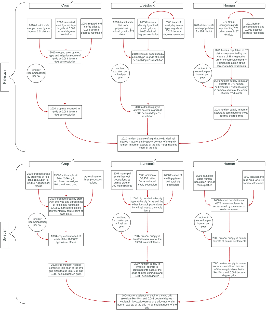
Figure 1. Data transformations from lower to higher resolution used to calculate nutrient balances in grids in Sweden and Pakistan. In Pakistan, the political scale (district) data for crops, livestock, and humans were converted to 0.083 decimal degree grids. In Sweden, the higher resolution crop data were transformed to include information of soil type and production region, and political scale (municipal) data for livestock and human were converted to farm livestock type and numbers, and human population to human settlement locations. All these datasets were then converted into crop nutrient needs and excreta nutrient supply and then into the gridded nutrient balances in each country.

Data Transformations and Calculations of Nutrient Balances in Grids

Pakistan

In Pakistan, we proportionally allocated total district cropped areas in 2010 (PBS, 2012) according to the distribution of crops in 2000 (FAO/IIASA, 2010) as shown in Equation (1) of Table 1, and similarly allocated district animal population data (PBS, 2012) as shown in Equation (2) in Table 1, and human population data (BOS, 2010, 2011, 2013, 2014) as shown in Equation (3) in Table 1 for 2010 according to spatially explicit gridded data (Robinson and Conchedda, 2011; Robinson et al., 2014). Before assigning district livestock population values to grids, we changed the spatial resolution of the gridded livestock data from 0.017 decimal degrees to 0.083 decimal degrees to bring it to the same spatial resolution as the crop data (ESRI, 2017). Assigning weighted human population values to grids was more complicated than for crops and animals. There were 383 sets of contiguous 0.0083 decimal degree grids representing major cities and towns¹ (Robinson and Conchedda, 2011). These cities and towns represented the population found in only 87 of the 124 districts in Pakistan (SI Figure 1). For the distribution of human population within the 87 districts that did have urban land use in the gridded dataset, we assumed that a larger urban area translated to a higher population density. As such we weighted the distribution of a district's population according to the area/size of the city as opposed to allocating an equal amount of the population to each grid that was considered urban using the following these steps:

• Converted each set of contiguous grids into separate polygon shapefile with ArcGIS (ESRI, 2016b) to create a “city”

• Calculated the area of each polygon shapefile, which then represented the size of a city or a town in Pakistan

• Used Equation (3) in Table 1 to allocate district human population (BOS, 2010, 2011, 2013, 2014) to human settlements according to the size of the cities in a district

• Allocated the excreta in each settlement to the 0.083 grid where the center point of the city was located

TABLE 1

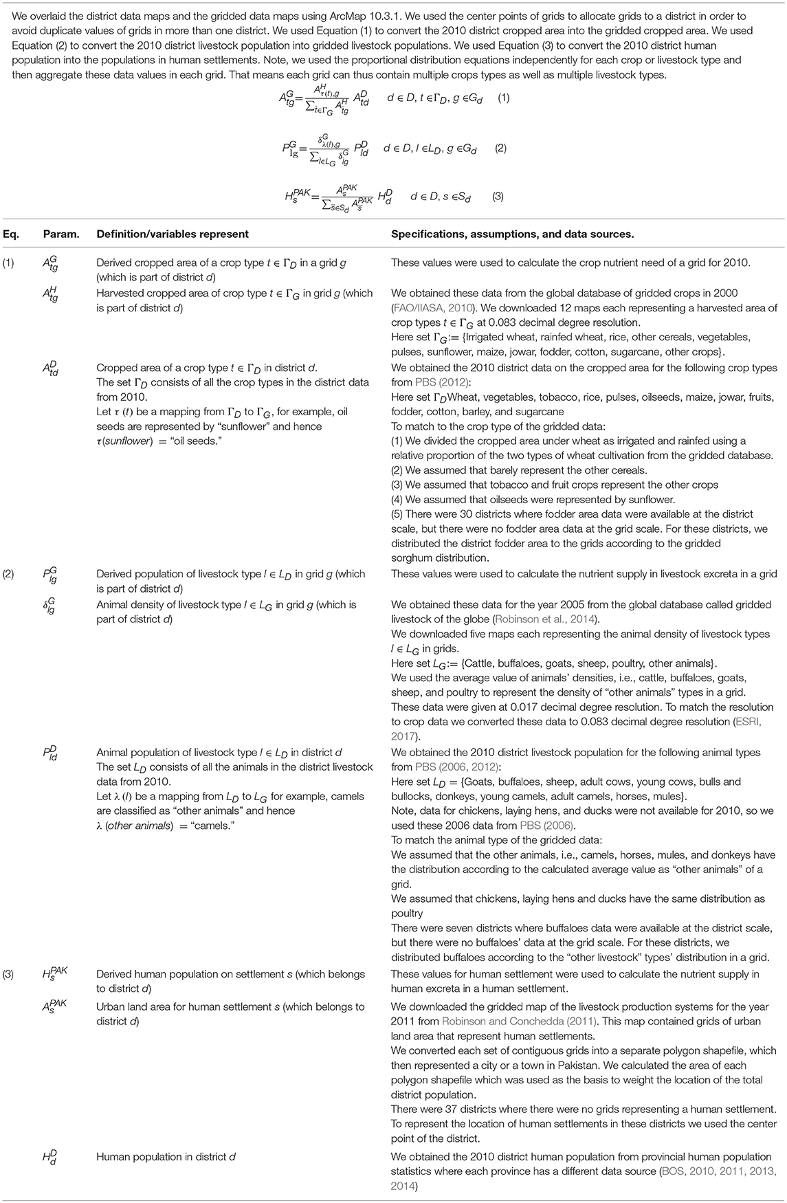
Table 1. Equations, data, and assumptions used to transform Pakistan low-resolution district cropped area, livestock, and human populations to higher resolution gridded data.

For the districts with no gridded urban land use (SI Figure 1), but where we knew there was human population, we used the center point of a district to represent the location of the entire population of a district (which is then equivalent to a human settlement in the equations below).

We converted the gridded cropped area data into crop nutrient needs using Equation (4):

$\begin{array}{ll}{C}_g^n={{\displaystyle \sum }}_{t\in {\Gamma }_D}{A}_{tg}^G{R}_{tg}^{n}g\in G,n\in \left\{N,P,K\right\}& (4)\end{array}$

where $C_g^n$is the total crop fertilizer need (in kg) of nutrient n in a grid g, $A_{tg}^G$ is the total cropped area (in ha) of crop type t grown in a grid g (from Equation 1), and $R_{tg}^n$ is the recommended fertilizer application rate (kg/ha) of nutrient n to crop type t grown in a grid g. For specific numbers of $R_{tg}^n$ see SI Table 1 which we obtained from Ashiq (2010) and FAO (2004).

We converted the gridded livestock data into livestock excreta nutrients using equation (5):

$\begin{array}{ll}{Q}_g^n={{\displaystyle \sum }}_{l\in L_D}{P}_{lg}^G{e}_l^n(1-v^n)g\in G,n\in \left\{N,P,K\right\}& (5)\end{array}$

where $Q_g^n$is the total quantity of nutrient n (in kg) in excreta in a grid g, $P_{lg}^G$ is the total number of individuals of livestock type l in a grid g (from Equation 2), and $e_l^n$ is the coefficient of excretion of nutrient (kg) n per individual of livestock type l; for specific numbers of $e_l^n$, see SI Table 2 which we obtained from Gerber et al. (2005). Parameter vⁿ is the gaseous loss of nutrient n during storage and field application of excreta which is only relevant for N (Bouwman et al., 1997).

We converted human population at human settlements into nutrients in human excreta using Equation (6):

$\begin{array}{ll}E{X}_s^n=H_s^{PAK}{e}^n(1-v^n)s\in S^{PAK},n\in \left\{N,P,K\right\}& (6)\end{array}$

where $E{X}_s^n$ is the total quantity of nutrient (in kg) n in human excreta at a human settlement s, $H_s^{PAK}$ is the total number of individuals at a human settlement s (from Equation 3), and eⁿ is the coefficient of excretion of nutrient (in kg) n per human individual per year. For specific numbers of eⁿ, see SI Table 2, which we obtained from Jönsson and Vinnerås (2004). Finally, vⁿ is the gaseous loss of nutrient n during storage and field application of excreta (which we assumed was equvalent to dairy cattle Bouwman et al., 1997). Here we do not consider losses of N or P associated with wastewater treatment for human excreta which typically results in only 5–40% of excreted N and 95% of P being found in sludge (Cohen, 2000). An improvement on our calculations and model would be to use specific wastewater treatment plant locations and nutrient emissions, but at this stage, considering limitations that would arise with estimating rural population emissions and data availability, we have opted to keep a per person excreta factor.

To integrate the nutrient supply found in human excreta from human settlements into one total value per grid, we used the center point of each settlement and allocated the full value of that settlement to the grid in which the center point fell (SI Figure 1). If there were multiple human settlements in a grid, we added those together to obtain one value per grid. Consequently, if a settlement overlapped multiple grids the value was not proportionally allocated between grids.

We used Equation (7) to calculate the nutrient balance of the grids in Pakistan:

$\begin{array}{ll}{B}_g^n={{\displaystyle \sum }}_{s\in S_g}E{X}_s^n+Q_g^n{-C}_g^{n}g\in G,n\in \left\{N,P,K\right\}& (7)\end{array}$

where $B_g^n$ is the balance of nutrient (in kg) n in grid g, S_g is a set of all human settlements that belongs to a specific grid g, $\sum _{s\in S_g}E{X}_s^n$ is the sum of human excreta nutrient n of human settlements s (in grid g), $Q_g^n$ is the total quantity of nutrient n in livestock excreta in grid g, and $C_g^n$ is the total crop need of nutrient n in grid g.

Sweden

In Sweden, we used the same proportional allocation approach as in Pakistan to combine the datasets, but we worked with much higher resolution base information. Spatial crop data were available at the field scale in 2008, expressed as 1 226 153 agricultural blocks with the crop-specific cultivated areas in each block (JBV, 2018a, data available upon request from Jordbruksverket). The agricultural blocks thus required no further resolution-transformation other than summarizing the information at the larger grid resolution for comparison with Pakistan. However, like in Akram et al. (in press), we incorporated the soil type and agricultural production region information to each agricultural block² to adjust fertilizer recommendations for crop types (Albertsson, 2007) using 10 km^*10 km grid-map on soil type data (Swedish Board of Agriculture, 2017) and the map of three production regions of Sweden (SI Figure 2). To do so, we used the center point of each agriculture block and overlaid them with soil type grids and agricultural region layers to assign each block a soil type/production-region/crop type combination.

For livestock, the Swedish government reported the 2008 location of 35 153 cattle farms with total cattle population on each farm (but not type of cattle) and 4,438 pig farms with total pig population [but not type of pig, JBV (2018b), data available upon request from Jordbruksverket]. There was no detailed spatial information on the locations and number of other animal types such as sheep, horses, and poultry. We proportionally allocated all other 2007 municipal livestock population types (and cattle types) according to the distribution of total cattle populations on cattle farms in that municipality and all pig types according to the distribution of total pig populations on pig farms in that municipality (Equation 8 in Table 2). This data transformation rests on two major assumptions: (1) the municipal livestock population was same in 2008 as it was in 2007, and (2) that production specialization is not separated by the type of animal; however, we still ensure that animal production areas were accurately represented by using total municipal numbers for each animal type when we allocated them to a farm location in a municipality.

TABLE 2

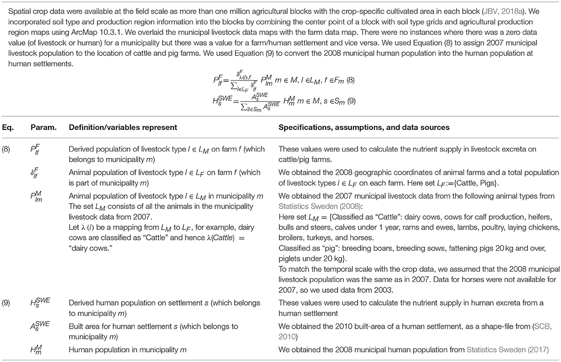
Table 2. Equations, data, and assumptions used to transform Swedish municipal scale livestock and human populations to farm and human settlement scale populations.

For humans, there were spatially explicit data for 2010 available as polygon shapefiles of 4,878 human settlements with a human population of at least 200 individuals (SCB, 2010), but not information for smaller settlements. To include the entire human population of a municipality in our calculations we distributed the municipal human population to human settlements like we did for Pakistan's districts (see Supplementary Information text where we demonstrate the numerical implication of allocating rural population according to build area by comparing these numbers to know urban population for one municipality in 2010; SI Table 5). We used the built-area of a settlement to proportionally distribute 2008 municipal population on the landscape (Equation 9 in Table 2).

We converted the cropped area of agricultural blocks into crop nutrient need using Equation (10), which is a slightly modified version of Equation (4):

$\begin{array}{ll}{C}_b^n={{\displaystyle \sum }}_{t\in {\Gamma }_B}{A}_{tb}^{SWE}{R}_{tb}^{n}b\in B,n\in \left\{N,P,K\right\}& (10)\end{array}$

where $C_b^n$is the total crop need of nutrient (in kg) n in an agricultural block b, Set Γ_B consists of all crop types in the block data (JBV, 2018a), $A_{tb}^{SWE}$ is the total cropped area (in ha) of crop type t grown in an agricultural block b (JBV, 2018a), and $R_{tb}^n$ is the recommended fertilizer rate of nutrient n to crop type t grown in an agricultural block b. For specific numbers of $R_t^n$ see SI Table 3A which we mainly obtained from Albertsson, 2007).

We converted the farm livestock data into livestock excreta supply using Equation (11), which is a slightly modified version of Equation (5):

$\begin{array}{ll}{Q}_f^n={{\displaystyle \sum }}_{l\in L_M}{P}_{lf}^F{e}_l^n(1-v^n)f\in F,n\in \left\{N,P,K\right\}& (11)\end{array}$

where $Q_f^n$is the total quantity (in kg) of nutrient n in livestock excreta at a livestock farm f, $P_{lf}^F$ is the total number of individuals of livestock type l at farm f (from Equation 8), and $e_l^n$ is the coefficient of excretion (in kg) of nutrient n per individual of livestock type l. For specific numbers of $e_l^n$, see SI Table 4 which we mainly obtained from (Albertsson, 2007). Finally, vⁿ is the gaseous loss of nutrient n during storage and field application of excreta (Bouwman et al., 1997).

We converted human population in human settlements in Sweden into human excreta (Equation 6) using $H_s^{SWE}$ from Equation (9). For the specific numbers of eⁿ for human excreta in Sweden see SI Table 4 which we obtained from Jönsson and Vinnerås (2004).

In order to combine crop nutrient needs and excreta nutrient supply in grids, we created two maps of hollow-grids: one of 0.083 decimal degree grids size, and other of 5 km^*5 km grid size (ESRI, 2016a). For crop nutrient needs, we used the center point of the agricultural blocks and allocated its value to the grid it fell in. The location of livestock farms was already represented as points and we thus subsequently allocated the full value of nutrient supply in livestock excreta to the grid in which the livestock farm (point) fell. In order to grid human excreta values from the human settlements into one total value per grid, we used the center point of each settlement and allocated the full value of that settlement to the grid in which the center point fell. If there were multiple agricultural blocks, livestock farms, or human settlements in a grid then we added these values together within each dataset.

We calculated the nutrient balance of the grids (each 5 km^*5 km and 0.083 decimal degree) in Sweden using Equation (12), which is a slightly modified version of Equation (7):

$\begin{array}{l}{B}_g^n={{\displaystyle \sum }}_{s\in S_g}E{X}_s^n+{{\displaystyle \sum }}_{f\in F_g}{Q}_f^n-{{\displaystyle \sum }}_{b\in B_g}{C}_b^n\\ g\in G,n\in \left\{N,P,K\right\}& (12)\end{array}$

where $B_g^n$ is the balance of nutrient n in grid g, $\sum _{s\in S_g}E{X}_s^n$ is the sum of human excreta nutrient n of human settlements s in grid g, $\sum _{f\in F_g}{Q}_f^n$ is the sum of the livestock excreta nutrient n of livestock farms f in grid g, and $\sum _{b\in B_g}{C}_b^n$ is the sum of the crop need of nutrient n of agricultural blocks b in grid g.

Optimized Transports

After calculating the nutrient balance of grids, we let the set ${\Delta }_{+}^n=\left\{g\in G:B_g^n>0\right\}$ represent all supply nodes (supply grids) and the set ${\Delta }_{-}^n=\left\{g\in G:B_g^n<0\right\}$ represent all crop nutrient need nodes (grids with deficits in nutrient n) for each grid-resolution in each country. In Pakistan we chose to optimize transportation of excess excreta between grids with respect to nutrient N, because we were interested in comparing it with the optimization of the political resolution study in Pakistan (Akram et al., 2018), while we optimized for nutrient P in Sweden to compare it to municipal resolution results (Akramet al., in press). The choice of N in Pakistan and P in Sweden were originally motivated by local conditions, notably that it is possible for Pakistan to decrease synthetic N fertilizer use and that in Sweden P is now coming to the forefront of management decisions. We then used Equation (13) to calculate the weight of surplus nutrients (as actual weight of manure and human excreta) for each grid-resolution in each country:

$\begin{array}{l}\text{Pak}:\\ W_g^n=\frac{B_g^n}{\left({\displaystyle {{\displaystyle \sum }}_{s\in S_g}E}{X}_s^n+Q_g^n\right)}\left({\displaystyle {\displaystyle \sum }_{l\in L_D}}{P}_{lg}^G{w}_l+{\displaystyle {\displaystyle \sum }_{s\in S_g}{H}_s^{PAK}}{w}_H\right)\\ g\in {\Delta }_{+}^n,n\in \{N,P,K\}& (\mathrm{13a})\end{array}$

$\begin{array}{l}\text{Swe}:\\ W_g^n=\frac{B_g^n}{\left({\displaystyle {{\displaystyle \sum }}_{s\in S_g}E{X}_s^n}+{\displaystyle {{\displaystyle \sum }}_{f\in F_g}{Q}_f^n}\right)}\left({\displaystyle {\displaystyle \sum }_{f\in F_g}{\displaystyle {\displaystyle \sum }_{l\in L_D}{P}_{lf}^F}}{w}_l+{\displaystyle {\displaystyle \sum }_{s\in S_g}{H}_s^{SWE}}{w}_H\right)\\ g\in {\Delta }_{+}^n,n\in \{N,P,K\}& (\mathrm{13b})\end{array}$

where $W_g^n$ is the weight of surplus of nutrient n as the actual weight of excreta in supply grid g, $P_{lg}^G$ and $P_{lf}^F$ are the number of animals of livestock type l in grids g and farms f, respectively, and w_l is the coefficient of the weight of manure from livestock type l and w_H is the coefficient of the weight of excreta (dry mass) from humans. For specific numbers of w_l and w_H see SI Table 2 for Pakistan and SI Table 4 for Sweden. We have opted to use these weights and not assign any specific excreta processing technology. Management decisions and technology selection would affect the weight (as well as nutrient availability) of the excreta that would be moved and selection of such technologies depend on a complex web on local conditions (e.g., laws, nutrient of interest, cost) which is beyond the scope of this analysis.

After calculating the actual weight of excreta associated with a surplus nutrient, we solved the Transportation Problem, a classical optimization problem, to calculate cost minimized transports of the surplus excreta nutrient to meet remaining crop nutrient need in deficit grids:

$\begin{array}{ll}minz=uDF{\displaystyle {\displaystyle \sum }_{i\in {\Delta }_{+}^n}}{\displaystyle {\displaystyle \sum }_{j\in {\Delta }_{-}^n}}{dis{t}_{ij}x}_{ij}/k_i& (14)\end{array}$

subject to

$\begin{array}{llll}{\displaystyle {\displaystyle \sum }_{i\in {\Delta }_{+}^n}}{x}_{ij}& =& B_i^{n}i\in {\Delta }_{+}^n& (15)\end{array}$

$\begin{array}{llll}{\displaystyle {\displaystyle \sum }_{j\in {\Delta }_{-}^n}}{x}_{ij}& \le & {-B}_j^{n}j\in {\Delta }_{-}^n& (16)\end{array}$

$\begin{array}{llll}{x}_{ij}& \ge & 0i\in {\Delta }_{+}^n,j\in {\Delta }_{-}^n& (17)\end{array}$

Variables x_ij represent the amount of nutrient n (in tons) to be sent from supply grid i to demand grid j, and the objective function (14) minimizes the total costs of transporting all the available surplus excreta. Parameter u is the unit cost for transportation of excreta, 0.02 US$ per ton and km for Pakistan (Teravaninthorn and Raballand, 2008) and 0.25 US$ per ton and km for Sweden (Greppa Näringen, 2012) and DF is distance factor to approximate the actual road distances given as the Euclidian distance between grids [we used 1.33 for both countries (Gonçalves et al., 2014)]. Parameter dist_ij is the Euclidian distance (in km) between center points for each grid, and parameter k_i is the concentration (the amount of nutrient n in each ton of manure, k_i = $4\frac{B_i^n}{W_i^n}$) at each sur-plus grid i. Constraint (15) makes sure that the entire surplus amount from grid i is distributed, and constraint (16) limits the amount of nutrient n received by each demand node j according to its deficit. Constraint (17) limits all transports to be positive.

Economic Analysis

In order to put the results of the optimization model into perspective with real-world costs and political priorities, we calculated a simple local profitability ratio for long-distance transported excreta, as well as constructed pre- and post-optimized scenarios to estimate the national effects of increased recycling on nutrient balances and potential monetary savings. We divided the total national transport cost (section Optimized Transports) by the total value of fertilizer³ transported in the excreta (N+P+K that matched crop needs in the deficit grids it was sent to) at each resolution in each country. A ratio below one indicates that the fertilizer value exceeds transport costs and thus is likely cost-effective and profitable (although this does not include processing and loading and unloading costs and thus is still a crude metric of profitability). Because both transportation costs and fertilizer values are locally specific, this ratio makes situations between countries easier to compare. This ratio, however, does not account for the full value of recycling as there is value in excreta reuse within grids as well, and as such we constructed the following scenarios for both countries at the decimal resolution:

Pre-optimized scenarios—We assumed that all excreta that could be recycled within the grids is the first choice to meet crop nutrient needs, followed by the use of synthetic fertilizers. This could result in an over-availability of synthetic fertilizer or a remaining gap for each of the nutrients. Excreta that required long-distance transport (i.e., outside of a grid) was assumed to be a surplus and not meeting crop needs in this scenario.

Post-optimized scenarios—We assumed that excreta that could be recycled within the grids plus the optimally transported excreta (i.e., excreta transported according to the optimal solution derived from equations in section Optimized Transports) were the first choice to meet crop needs. We then calculated the amount of synthetic fertilizer required to fully meet crop nutrient needs. We also account for the fact that there was over-application of non-optimally transported nutrients because of fixed nutrient stoichiometric ratios in excreta.

Comparing these pre- and post-optimized scenarios complements the profitability ratio by allowing us to estimate the value of recycling if it can reduce synthetic fertilizer application, as well as explicitly show where applying excreta (and thus by default optimizing transportation) for one nutrient may cause imbalances for another. We were further able to monetize the effect of post-optimized recycling scenarios by accounting for savings associated with ceasing over-application of synthetic fertilizers in addition to the fertilizer value of excreta itself. We then compared these savings with the cost of transport as well as the cost of purchasing additional synthetic fertilizers if crop needs could not be met with recycling and existing fertilizer use. We did so by calculating a ratio of savings and expenses where we divided the total NPK fertilizer savings values (all recycled manure value + over application of synthetic fertilizers) by the sum of the cost of transportation and unmet crop needs if to be met by synthetic fertilizer values. This ratio could then be interpreted as the proportion of costs associated with fertilization (transport of excreta and the additional synthetic fertilizers required to meet crop needs if synthetic fertilizer purchases in the pre-optimized scenario were insufficient) that can be covered with savings on synthetic fertilizers.

Results and Discussion

Spatial Patterns of Supply and Need Vary Between Sweden and Pakistan

Both Sweden and Pakistan exhibited agricultural specialization; areas of nutrient surplus and deficit were visible at the 0.083 decimal degree resolution (Figure 2). For all nutrients, Pakistan showed much higher nutrient needs (e.g., four times higher P need per hectare than in Sweden), which is likely related to climate differences and the associated multi-cropping and different crop choices possible in Pakistan (SI Table 6). Similarly, the average supply of P in excreta per ha in Pakistan was two times higher than in Sweden. Both countries showed distinct areas of concentrated excreta supply and crop need. Pakistan had high excreta nutrient supply along the western border, with some additional “hotspots” in the center and south-east parts of the country. These areas (over 144 kg N/ha) contained 27% of the national N excreta supply but only 6% of the arable area (SI Table 7). Higher crop nutrient needs, on the other hand, were concentrated in the middle and the eastern parts of the country, extending south along the Indus River. These crop nutrient need regions did not exhibit as striking a concentration on the landscape as with supply (e.g., 28% P need on 21% of the arable land area). In Sweden, excreta supply was concentrated in the south of the country and especially in big cities, such as Stockholm and Gothenburg (e.g., 11% of N supply could be attributed to 1% of the land area, and this was mostly cities, Figure 2 and SI Table 7). Crop nutrient needs were higher (more concentrated) in the middle of the country, along the northeast coast, and at the very southern tip of the country. These contrasting spatial patterns of supply and need unsurprisingly resulted in surplus and deficit areas in both countries.

FIGURE 2

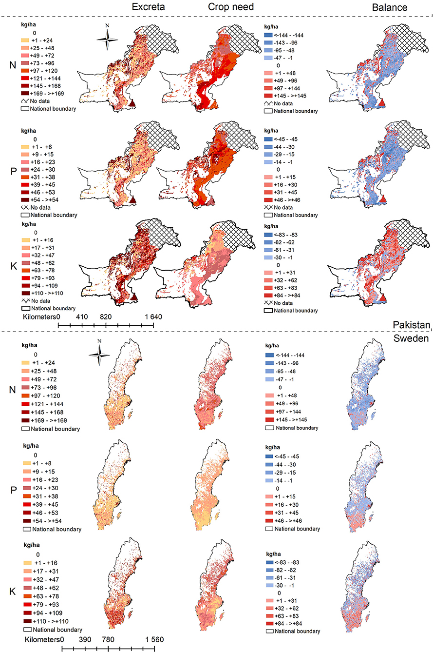
Figure 2. Spatial distribution of excreta nutrient supply, crop nutrient needs, and nutrient balances as nitrogen (N), phosphorus (P), and potassium (K) at the 0.083 decimal degree grid resolution in Pakistan (top three rows) and Sweden (bottom three rows).

At the national scale, the surplus and deficit patterns for nutrients differed. In both countries recycling all K could meet crop needs (even if transport is required). In Pakistan, although excreta could not fulfill all crop N and P needs, it could proportionally meet more of N than P crop needs (57% for N vs. 43% for P, Figure 5). In Sweden it was the opposite, a larger proportion of P needs could be met (45% N vs. 88% P, Figure 5). As such it made sense to optimize transportation for different nutrients in each country (Akram et al., 2018; Akram et al., in press).

Moving from political to decimal resolution spatial data did not yield a consistent pattern on surplus and deficits across nutrients between the two countries. In Pakistan, increasing resolution highlighted that there was land use specialization; at the decimal resolution 43% of grids showed N surpluses and 35% grids showed P surpluses, which is 18% higher for N, and 17% higher for P compared to the proportion of districts that exhibited a surplus (SI Table 8). Interestingly, in Sweden the patterns were reversed. Only 7% of the decimal grids had an N surplus, and 15% had a P surplus at the decimal resolution, which is actually 12% less than the proportion of municipalities that had an N and P surplus (SI Table 9). This Swedish trend may be linked to even more extreme specialization than in Pakistan, as so few grids accounted for the total surplus in Sweden. For K, increasing resolution in both countries decreased the proportion of land that exhibited nutrient surpluses.

Increasing Resolution Increases the Need for Transportation but Decreases Average Distances

The estimated amount of excreta which needed to be transported increased when higher resolution data was used in both countries (Figure 3A). Moving from political boundaries to decimal degrees increased the amount of N requiring transport by 12% in Pakistan and increased the amount of P requiring transport by 14% in Sweden. However, this increase represented a tripling for Pakistan but less than a doubling for Sweden. This may be related to differences between the Pakistani political resolution (average district area was 6,689 km²) and Swedish political resolution (average municipality area was 1,832 km²) so the increase to decimal degree was a less noticeable increase in Sweden. Further increasing the resolution to 5 km grids in Sweden did not substantially increase the amount of excreta P requiring transport (+4%). If we compare the effect of increasing resolution on the weight of excreta requiring transport instead of the quantity of nutrients, we obtain quite similar results. The weight of excreta requiring transport increased by 16% in Pakistan and 12% in Sweden going from political to decimal resolution, and another 4% increase to the 5 km resolution in Sweden (SI Figure 3). Although, the proportion of grids with surpluses in Sweden was less than in Pakistan (SI Tables 8, 9), a larger proportion of excreta needed to be transported out of the grids in Sweden than in Pakistan (Figure 3A); this points to Sweden's high level of agricultural specialization which is visible at all three resolutions (SI Table 9). In summary, using higher resolution data accounted for imbalances that not evident at lower resolution boundaries thus uncovers the fact that many shorter transport distances are required to balance crop needs and excreta supply.

FIGURE 3

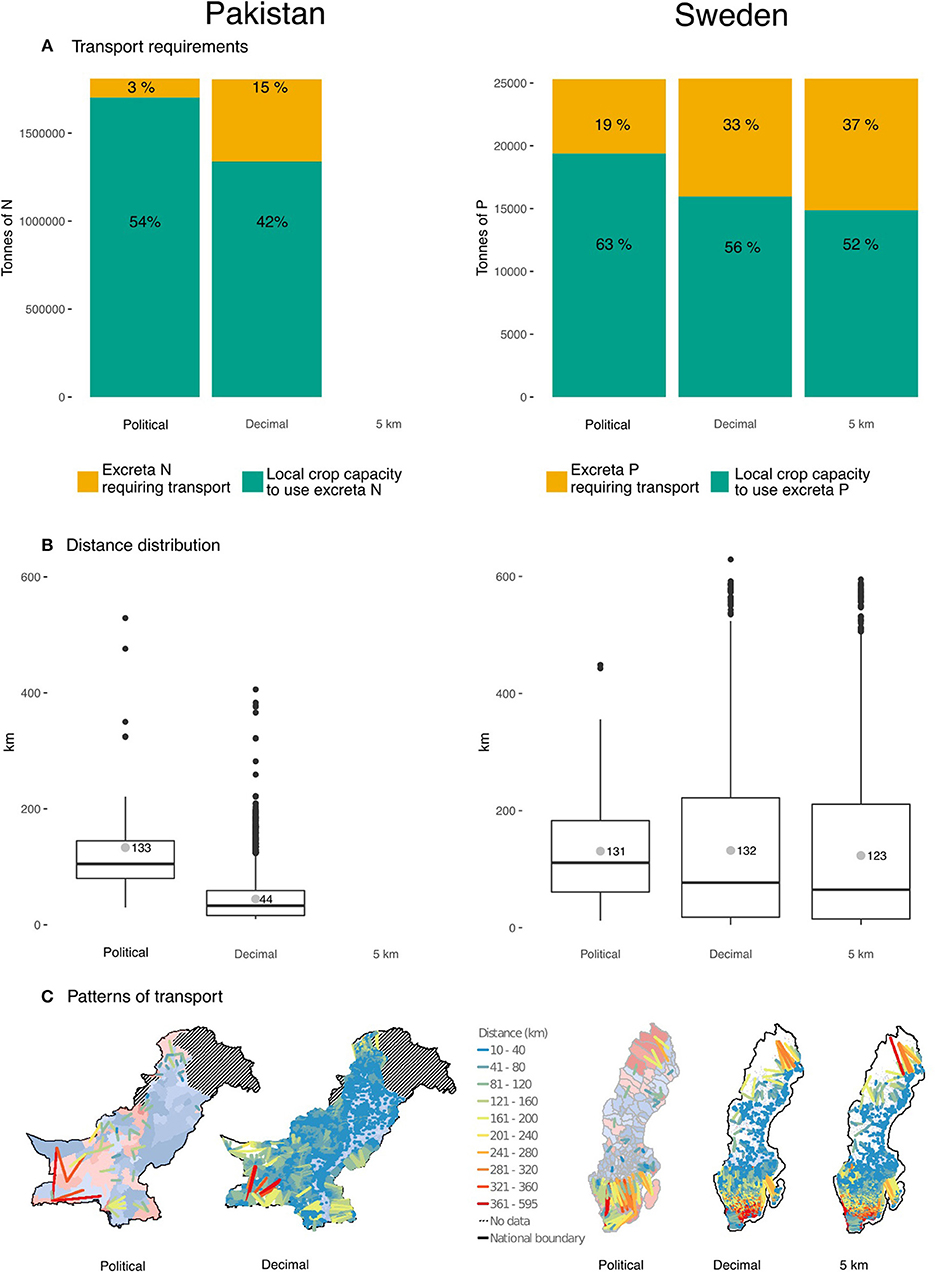
Figure 3. Effects of increasing resolution from political, to decimal, to 5 km scales on the transportation of surplus nutrients in terms of (A) the amount and percentage of the nutrient of interest (N for Pakistan and P for Sweden) requiring transport, (B) the spread of transport distances represented as mean (gray circles and stated value), median (center line), interquartile range (box representing 50% of the data), 1.5 times the interquartile range (whiskers), and outliers (black circles), and (C) the paths and distances of transportation on the landscape from surplus (light red) to deficit areas (light blue) color-coded from shorter (blue lines) to longer (red lines).

Increasing data resolution generally decreased average transport distances and changed transport patterns in both countries, but more in terms of distances for Pakistan and transport patterns for Sweden (Figures 3B,C). In Pakistan the average distance decreased 67% (from 133 to 44 km), the interquartile range and fence (1.5 times interquartile range) became smaller, but there were more long-range outliers than in Sweden (Figure 3B). In Sweden, the average distance actually increased from 131 to 132 km between political and decimal resolutions. The interquartile ranges increased, and so did the maximum distance when comparing the political resolution to the decimal and the 5 km grid resolutions. However, moving from decimal to 5 km resolution decreased the average distance by 9 km, thus still supporting the general premise that increasing resolution decreases average distances. Part of the different trend with increasing resolution between Sweden and Pakistan could, again, be linked to the base political boundary resolution, in addition to more agricultural specialization on the Swedish landscape. At the decimal resolution, Pakistan had a shorter average distance than Sweden. In Sweden, long-range transports were predominantly in the south-west part of the country at the political resolution but shifted to south-east at the decimal degree resolution. These required long-range transports then shifted back toward the south-west coast at the 5 km resolution (noting of course that there were fewer long-distance transports overall at the higher resolution). The perhaps unintuitive results of comparing distances, weights, and patterns of transport across scales and then between countries highlights that optimizing to minimize cost nationally does not mean that any one transport (or even average transport patterns) is optimal on its own.

Even with the highest resolution data we had available in each country, the average required transport distances were on the higher end of what existing studies have found to be cost-effective. Although drier poultry litter may be worthwhile transporting over 400 km (Sharpley et al., 2016), acceptable transport distance estimates for wetter manure never went much above 50 km in modeled and observational studies (Fealy and Schröder, 2008; Nowak et al., 2015). Our average transport distance in Pakistan was the lowest, at 44 km, but there were still a number of outlier transports as high as 400 km. In Sweden, the average transport distance was still above 100 km with 5 km grids. Like our numbers suggest, other studies have found that required transport distances to avoid over-fertilization with manure are higher than what is considered cost-effective under current pricing mechanisms. For example, for the Chesapeake Bay area of the USA, keeping below P standards for manure application to fields would require increasing transport distances within farms and counties, but most importantly increasing transport among counties to an average of 190 km if farmers would accept applying 60% of their fertilizer as manure (it is currently 17% for corn, Ribaudo et al., 2003). Still, longer average transports could be realistic and profitable; site-specific costs; and incentive structures (e.g., laws preventing over-application of manure or land filling of organic waste) must also be accounted for. It is also worth examining costs at the national scale to determine if the benefit of some of the shorter distance transports can outweigh the costs of longer distance ones under current pricing mechanisms.

Local Pricing Conditions Favor Recycling in Pakistan More Than in Sweden

Like with the total amount of excreta requiring transport (Figure 3A), total distance increased with increasing resolution, but costs did not scale with these increases proportionally; in other words, costs increased but not as quickly as distance or weight (Table 3). In Pakistan, the total transport distance increased 44 times from political to decimal resolution, but the total transport cost increased 1.6 times. In Sweden, costs increased 1.4 times but distance increased less than in Pakistan, only 14 times; which again could be related to higher political resolution and agricultural specialization in Sweden. Interestingly, moving from decimal degree to 5 km grids decreased estimated total costs, although total distance and weight did increase (Table 3, SI Figure 3). This would imply that there were fewer required long-distance travel routes with heavy loads. We can see a smaller interquartile range associated with the optimization of 5 km resolution data and fewer long-distance outliers compared to the interquartile range of the decimal degree resolution (Figure 3B), which does support the idea of fewer long-distance transports contributing to these savings in the 5 km resolution model.

TABLE 3

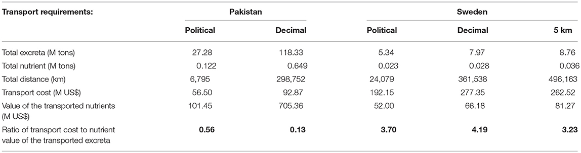
Table 3. Total national weight, distance, and cost requirements associated with optimally transported surplus excreta at different resolutions in Pakistan and Sweden.

Costs are not only related to distance and weight, but also local pricing mechanisms which make recycling more or less favorable. One way to look at the cost-effectiveness of recycling between countries is to compare the cost of transport to the value of fertilizers being transported as excreta (expressed as a ratio in Table 3). In Pakistan transporting excess excreta seemed economically favorable even at the political resolution with a ratio value below 1 (Akram et al., 2018), but dropped even further at the decimal resolution; 13% of the fertilizer value being transported could cover the entire cost of transportation (Table 3, Figure 4). For Sweden, transportation at all resolutions seemed unfavorable, but the ratios actually increased from political to decimal resolution, and then decreased overall at the 5 km resolution (Table 3, Figure 4). This sharp increase in the ratio at the decimal scale seems to be related to the value (or lack thereof) related to N and K transported alongside P. If we only account for P fertilizer value in transported excreta (SI Figure 4) then the ratio steadily decreases with increasing resolution, as one would expect. In other words, at the decimal resolution less N and K were applied to areas that had crop need for it. It is important to note that not all individual transports in the Swedish optimization model are economically unfavorable: 34% of transports (1,374 connections between grids out of the 4,020 modeled) have a ratio below the break-even point based on only the P fertilizer value transported. This means that 17% of the surplus excreta weight actually represents 10% of the distance and only 2% of the costs associated with transportation, but 31% of the P fertilizer value. Still, in order to make total nutrient recycling in Sweden cost-effective under current excreta supply and crop need distribution, other factors would need to change. This could be directly achieved with decreasing transport costs (perhaps associated with different fuels or higher fuel efficiency) or with increasing synthetic fertilizer prices (through taxation or market forces), making excreta more valuable. This could also potentially be achieved if we were to extract energy from excreta before land application (e.g., biogas). In other words, this would involve accounting for the full value of recycling, both direct use value as well as the avoidance of pollution.

FIGURE 4

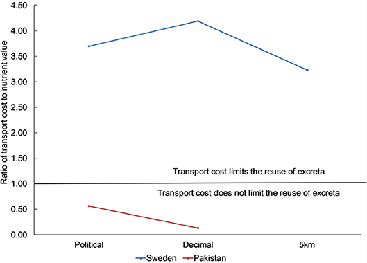
Figure 4. Effect of increasing spatial resolution on the relative transport costs of surplus excreta nutrients to the value of those nutrients if they were purchased as synthetic fertilizer in Sweden (blue, higher line) and Pakistan (orange, lower line).

In both countries, implementing optimized recycling resulted in less discrepancies between nutrient supply and crop nutrient needs and potential for reducing expenditures on synthetic fertilizers. In Pakistan, recycling all excreta could decrease synthetic N needs to only 43% of its current use, but there remain unmet crop P and K needs (Figure 5 and Table 4). In fact, a significant amount of synthetic N use could potentially be cut even in the pre-optimized scenario. In Sweden, the use of synthetic N would be cut by 11%, synthetic P by 67%, and synthetic K by 11% by recycling all excreta (Figure 5). Optimized transportation could also reduce the gap between nutrient needs and national nutrient supply. In Pakistan, transportation between grids could reduce the gap between P crop need and P supply by 10%, and the gap between K crop need and K supply by 7%. In Sweden, the post-optimization scenario eliminated the gap between P crop need and P supply. Although the application of surplus excreta in deficit areas optimized for only one nutrient did result in some over-application for the non-optimized nutrients, the magnitude of that over application is much smaller than in the pre-optimized scenarios (Figure 5).

FIGURE 5

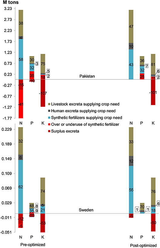
Figure 5. National nutrient balances associated with scenarios of pre- and post-optimized transport of surplus excreta at decimal degree resolution in Pakistan (top panel) and Sweden (bottom panel). The height of each bar above zero represents total crop nutrient need, while the height below zero represents the total nutrient surplus given the assumptions presented in section Economic Analysis. Colors represent the nutrient source used to fill the crop nutrient need above zero while colors below zero represent the type of nutrient surplus. A gap between crop nutrient need and supply is designated as red above 0. The numbers in each colored column section represent the percentage of crop need that a source fulfills, where negative numbers (below the zero line) represent the surplus also expressed as a percentage of crop need.

TABLE 4

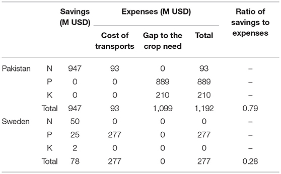
Table 4. Savings on synthetic fertilizers (millions of US dollars) associated with decimal resolution optimized recycling of excreta vs. transport costs incurred and additional costs for synthetic fertilizers to meet crop nutrient need in Pakistan and Sweden.

At the national level, accounting for potential savings associated with local and long-distance recycling still did not make recycling seem cost-effective in Sweden without accounting for pollution abatement, while in Pakistan recycling seemed even more beneficial. For Pakistan, savings on synthetic fertilizers had the potential to contribute to covering the cost of transportation and part of the additional synthetic fertilizer costs required to close yield gaps; the savings on synthetic N fertilizers would not only cover transportation costs of excreta but also 78% of money required to meet P, and K crop needs with synthetic fertilizers in the post-optimization scenario (Table 4). Our cost and savings estimates however were simple and did not account for the potentially significant costs associated with processing excreta, which is paramount to eliminate pathogen and other contaminant exposure (Bloem et al., 2017), costs associated with loading and unloading trucks (Ghafoori et al., 2007), or laws and public perceptions they may facilitate or hinder recycling, especially in the case of human excreta (Metson et al., 2018; Öberg and Mason-Renton, 2018). In Sweden, the savings on the synthetic fertilizers would only cover 28% of the transportation costs for redistributing surplus excreta. Considering that pollution does have a financial cost however, the expenses associated with increased recycling might be worth baring. In England and Whales, freshwater eutrophication has been estimated to cost up to 160 million USD per year (Pretty et al., 2003), while in the USA health and environmental costs associated with N pollution (air and water) are estimated at 210 billion USD per year (Sobota et al., 2015). Around the Baltic Sea, the willingness to pay (as a proxy for the costs associated with poor water quality) to reduce Baltic eutrophication varies but is actually highest in Sweden (Hyytiäinen et al., 2015). Accounting for nutrient losses to the Baltic Sea, lakes, and groundwater associated with areas of excreta accumulation may change the picture for the cost-effectiveness of excreta recycling (Hyytiäinen et al., 2015; Gren and Elofsson, 2017).

Concluding Remarks

In summary, increasing the resolution of input data to a model optimizing the cost of recycling excreta to meet remaining crop nutrient needs after local recycling did affect the amount, distance, patterns, and costs associated with transportation in both Pakistan and Sweden; but the cost-effectiveness associated with local pricing contributed more to the differences between the countries than anything else. In both cases the amount of excreta requiring transport increased with increasing spatial resolution, but not at the same rate. Total distances also increased although the average distance of any one transport decreased (and even slightly increased at the decimal scale in Sweden). The average distance was much lower in Pakistan, likely due to less agricultural specialization than in Sweden. Increasing to 5 km resolution in Sweden did decrease the cost of transportation even though total distance increased. Increasing resolution in both countries decreased the ratio of cost to value, potentially making it easier to make a case for a profitable recycling industry. However, the ratio of cost to value was more unfavorable at the decimal resolution than at the municipal or 5 km resolutions, in large part because less N and K being moved were meeting crop needs. At all resolutions, recycling excreta under our model assumptions always came out as economically favorable in Pakistan while it did not in Sweden. This means that although optimizing transport will be important, considering the social, technological, and ecological context surrounding these transports will be essential to more sustainable nutrient management. Next steps would thus include better integration of not only the real-world costs associated with processing of waste and transportation, but the monetary benefits associated with increased recycling beyond nutrient value (e.g., energy or pollution abatement).

The methods, datasets, and results presented here are a significant step toward being able to make informed decisions about what it would take for countries to create a circular nutrient economy, especially as more standardized spatially and temporally resolved data become available. The high resolution maps in both countries more accurately show where there are nutrient imbalances that require judicious management. There are many social and ecological constraints, which if represented spatially, could be integrated into the models presented here to help inform farmers and decision makers even more. For example, human and animal excreta are often regulated and handled separately. Although, the current model gives a good overview of the potential of both resources, further development in the model could integrate different handling/processing realities and preferences. For instance, if human and animal excreta were treated separately in the model one could track which farmland would “optimally” receive it and see if this matches the laws and regulations in place. Similarly, the production of excreta and crop nutrient needs often do not coincide. As such, storage and processing of excreta will often be necessary to ensure nutrients can be applied when they are needed, which could affect both the weight and nutrient content of recycled organic waste products. Processing may not only create costs, but also additional benefits, such as energy through biogas production, that could make the circular economy more profitable. The current model operates at an annual scale, but a sub-annual component could potentially be added to try and optimally select locations for excreta storage and then subsequent application to crops. Even if such data is not available nationally, the model and approach presented here can be downscaled to work with local stakeholders who may have access to relevant data, including locally appropriate technologies for processing of organic waste.

Data Availability

All datasets generated for this study are included in the manuscript and/or the Supplementary Files.

Author Contributions

UA collected and analyzed data and contributed to the writing. N-HQ conducted optimization modeling and reviewed the manuscript. UW and KT secured the funding for this project, conceptualized initial study, and reviewed the manuscript. GM reviewed and corrected the methodological design of the study, as well as led framing, figure design, and writing of the manuscript.

Funding

We are grateful to FORMAS, the Swedish research council for sustainable development, for funding this work. Grant: 992023 UW. FORMAS 942-2016-69.

Conflict of Interest Statement

The authors declare that the research was conducted in the absence of any commercial or financial relationships that could be construed as a potential conflict of interest.

Supplementary Material

The Supplementary Material for this article can be found online at: https://www.frontiersin.org/articles/10.3389/fsufs.2019.00050/full#supplementary-material

Footnotes

1. ^The extent of urban areas in the base gridded dataset was derived from a combination of the Global Rural-Urban Mapping Project (GRUMP) dataset and the global land cover GLC 2000 urban class based on night satellite imagery using the Defense Meteorological Satellite Program operational linescan system.

2. ^We identified and assigned each block a crop production region and the soil class of P-AL and K-AL. The assigning was used to match the fertilizer recommendation rates, which were different for a crop based on the region or the soil class in which the crop was being grown (SI Table 3A).

3. ^For Pakistan, we used the same values as in Akram et al. (2018) for the market value of 1 kg of synthetic fertilizer nutrient which were obtained from the National Fertilizer Development Center. For Sweden we use the same values as in Akram et al. (in press) which were obtained from Greppa Näringen (2008).

References

Akram, U., Metson, G. S., Quttineh, N., and Wennergren, U. (2018). Closing Pakistan's yield gaps through nutrient recycling. Front. Sustain. Food Syst. 2, 1–14. doi: 10.3389/fsufs.2018.00024

CrossRef Full Text | Google Scholar

Akram, U., Quttineh, N-H., Wennergren, U., Tonderski, K., and Metson, G. S. (in press). Enhancing nutrient recycling from excreta to meet crop nutrient needs in Sweden—a spatial analysis. Sci. Rep. doi: 10.1038/s41598-019-46706-7

CrossRef Full Text

Albertsson, B. (2007). Riktlinjer för gödsling och kalkning 2008. Available at: https://www2.jordbruksverket.se/webdav/files/SJV/trycksaker/Pdf_rapporter/ra07_22.pdf (accessed June 19, 2019).

Google Scholar

Ashiq, M. (2010). Punjab main 75 faslon key Munafah bakhash kashat kari (Profitable cultivation of 75 crops in Punjab). Plant physiology section, Nizamat Amoor-e-kashat kari (Agronomy), Ayub Agriculture Research Institute, Faisalabad, Pakistan.

Google Scholar

Bergendahl, J. A., Sarkis, J., and Timko, M. T. (2018). Transdisciplinarity and the food energy and water nexus: ecological modernization and supply chain sustainability perspectives. Resour. Conserv. Recycl. 133, 309–319. doi: 10.1016/j.resconrec.2018.01.001

CrossRef Full Text | Google Scholar

Bloem, E., Albihn, A., Elving, J., Hermann, L., Lehmann, L., Sarvi, M., et al. (2017). Contamination of organic nutrient sources with potentially toxic elements, antibiotics and pathogen microorganisms in relation to P fertilizer potential and treatment options for the production of sustainable fertilizers: a review. Sci. Total Environ. 607–608, 225–242. doi: 10.1016/j.scitotenv.2017.06.274

PubMed Abstract | CrossRef Full Text | Google Scholar

BOS (2010). Punjab Development Statistics 2010. Bureau of Statistics Punjab, Lahore. Available online at: http://www.bos.gop.pk/system/files/Dev-2010.pdf (accessed June 19, 2019).

Google Scholar

BOS (2011). Development Statistics of Balochistan 2011-12. Area and Population Table 6. Bureau of Statistics Balochistan, Planning and Development Department, Quetta. Available online at: https://balochistan.gov.pk/index.php?option=com_docman&task=cat_view&gid=1277&Itemid=677&limitstart=15 (accessed June 19, 2019).

Google Scholar

BOS (2013). Development Statistics of Khyber Pakhtunkhwa 2011-12. Bureau of Statistics Khyber Pakhtunkhwa, Peshawar. Available online at: http://kpbos.gov.pk/files/1385537977.pdf (accessed August 16, 2018).

Google Scholar

BOS (2014). Development statistics of Sindh 2014. Sindh Bureau of Statistics, Kehkashan Clifton. Available online at: http://sindhbos.gov.pk/wp-content/uploads/2014/09/DS-2014.pdf (accessed June 19, 2019).

Google Scholar

Bouwman, A. F., Lee, D. S., Asman, W. A. H., Dentener, F. J., Hoek, K. W., Van Der Olivier, J. G. J., et al. (1997). A global high-resolution emission inventory for ammonia. Glob. Biogeochem. Cycles 11, 561–587. doi: 10.1029/97GB02266

CrossRef Full Text | Google Scholar

Cohen, Y. (2000). Nutrient Recovery from Wastewater. Available online at: http://www.vaxteko.nu/html/sll/slu/ex_arb_vaxtnaringslara/EVN119/EVN119.HTM (accessed June 19, 2019).

Google Scholar

Cordell, D., Turner, A., and Chong, J. (2015). The hidden cost of phosphate fertilizers: mapping multi-stakeholder supply chain risks and impacts from mine to fork. Glob. Chang. Peace Secur. 27, 323–343. doi: 10.1080/14781158.2015.1083540

CrossRef Full Text | Google Scholar

Diaz, R. J. (2001). Overview of hypoxia around the world. J. Environ. Qual. 30, 275–281. doi: 10.2134/jeq2001.302275x

PubMed Abstract | CrossRef Full Text | Google Scholar

EC (2016). Circular Economy : New Regulation to boost the use of organic and waste-. Available online at: http://europa.eu/rapid/press-release_IP-16-827_en.pdf (accessed June 19, 2019).

Google Scholar

Englande, A. J. Jr., and Reimers, R. S. (2001). Biosolids management–sustainable development status and future direction. Water Sci. Technol. 44, 41–46. doi: 10.2166/wst.2001.0575

PubMed Abstract | CrossRef Full Text | Google Scholar

ESRI (2016a). Create Fishnet. Available online at: http://desktop.arcgis.com/en/arcmap/10.3/tools/data-management-toolbox/create-fishnet.htm (accessed September 24, 2018).

Google Scholar

ESRI (2016b). Raster to Polygon. Available online at: http://desktop.arcgis.com/en/arcmap/10.3/tools/conversion-toolbox/raster-to-polygon.htm (accessed June 19, 2019).

Google Scholar

ESRI (2017). Cell Size and Resampling in Analysis. Available online at: http://desktop.arcgis.com/en/arcmap/latest/extensions/spatial-analyst/performing-analysis/cell-size-and-resampling-in-analysis.htm# (accessed June 19, 2019).

Google Scholar

FAO (2004). Fertilizer use by Crop in Pakistan. Rome Available online at: http://www.fao.org/tempref/docrep/fao/007/y5460e/y5460e00.pdf (accessed June 19, 2019).

Google Scholar

FAO/IIASA (2010). Crop Harvested Area, Yield and Production. Available online at: http://gaez.fao.org/Main.html# (accessed June 19, 2019).

Google Scholar

Fealy, R., and Schröder, J. J. (2008). Assessment of Manure Transport Distances and their Impact on Economic and Energy Costs. York: IFS. 228.

Google Scholar

Flotats, X., Bonmatí, A., Fernández, B., and Magr,í, A. (2009). Manure treatment technologies: on-farm versus centralized strategies. NE Spain as case study. Bioresour. Technol. 100, 5519–5526. doi: 10.1016/j.biortech.2008.12.050

PubMed Abstract | CrossRef Full Text | Google Scholar

Freeze, B. S., and Sommerfeldt, T. G. (1985). Breakeven hauling distances for beef feedlot manure in southern Alberta. Can. J. Soil Sci. 65, 687–693. doi: 10.4141/cjss85-074

CrossRef Full Text | Google Scholar

Geissdoerfer, M., Savaget, P., Bocken, N. M. P., and Hultink, E. J. (2017). The circular economy – a new sustainability paradigm? J. Clean. Prod. 143, 757–768. doi: 10.1016/j.jclepro.2016.12.048

CrossRef Full Text | Google Scholar

Gerber, P., Chilonda, P., Franceschini, G., and Menzi, H. (2005). Geographical determinants and environmental implications of livestock production intensification in Asia. Bioresour. Technol. 96, 263–276. doi: 10.1016/j.biortech.2004.05.016

PubMed Abstract | CrossRef Full Text | Google Scholar

Ghafoori, E., Flynn, P. C., and Feddes, J. J. (2007). Pipeline vs. truck transport of beef cattle manure. Biomass Bioenergy 31, 168–175. doi: 10.1016/j.biombioe.2006.07.007

CrossRef Full Text | Google Scholar

Ghisellini, P., Cialani, C., and Ulgiati, S. (2016). A review on circular economy: the expected transition to a balanced interplay of environmental and economic systems. J. Clean. Prod. 114, 11–32. doi: 10.1016/j.jclepro.2015.09.007

CrossRef Full Text | Google Scholar

Gonçalves, D. N. S., de MoraisGonçalves, C., de Assist, T. F, and da Silva, M. A. (2014). Analysis of the difference between the euclidean distance and the actual road distance in Brazil. Transp. Res. Procedia 3, 876–885. doi: 10.1016/j.trpro.2014.10.066

CrossRef Full Text | Google Scholar

Gren, I.-M., and Elofsson, K. (2017). Credit stacking in nutrient trading markets for the Baltic Sea. Mar. Policy 79, 1–7. doi: 10.1016/j.marpol.2017.01.026

CrossRef Full Text | Google Scholar

Greppa Näringen (2008). Verktyg i Miljöarbetet Behövs mer än någonsin! Available online at: http://www.greppa.nu/download/18.37e9ac46144f41921cd1a92d/1402565001964/2008_Mar_GreppaNYTT.pdf (accessed April 14, 2019).

Google Scholar

Greppa Näringen (2012). Praktiska Råd: Din Stallgödsel är Värdefull. 1–6. Available online at: http://www.greppa.nu/download/18.37e9ac46144f41921cd1a724/1402315666376/Praktiska_råd_Nr_5_Stallgödsel_5.pdf (accessed June 19, 2019).

Google Scholar

Hamilton, D. P., Salmaso, N., and Paerl, H. W. (2016). Mitigating harmful cyanobacterial blooms: strategies for control of nitrogen and phosphorus loads. Aquat. Ecol. 50, 351–366. doi: 10.1007/s10452-016-9594-z

CrossRef Full Text | Google Scholar

Harrison, J. A., Bouwman, A. F., Mayorga, E., and Seitzinger, S. (2010). Magnitudes and sources of dissolved inorganic phosphorus inputs to surface fresh waters and the coastal zone: a new global model. Glob. Biogeochem. Cycles 24, 832–839. doi: 10.1029/2009GB003590

CrossRef Full Text | Google Scholar

Horritt, M. S., and Bates, P. D. (2001). Effects of spatial resolution on a raster based model of flood flow. J. Hydrol. 253, 239–249. doi: 10.1016/S0022-1694(01)00490-5

CrossRef Full Text | Google Scholar

Hyytiäinen, K., Ahlvik, L., Ahtiainen, H., Artell, J., Huhtala, A., and Dahlbo, K. (2015). Policy goals for improved water quality in the baltic sea: when do the benefits outweigh the costs? Environ. Resour. Econ. 61, 217–241. doi: 10.1007/s10640-014-9790-z

CrossRef Full Text | Google Scholar

JBV (2018a). Jordbruksblock. Available online at: http://www.jordbruksverket.se/etjanster/etjanster/etjansterforstod/kartorochgis/inspiretjanster/laddanerkartskikt.4.2c4b2c401409a334931bf0e.html (accessed June 19, 2019).

Google Scholar

JBV (2018b). Produktionsplatser för Djurhållning. Available online at: http://www.jordbruksverket.se/etjanster/etjanster/etjansterforstod/kartorochgis/inspiretjanster/laddanerkartskikt.4.2c4b2c401409a334931bf0e.html (accessed June 19, 2019).

Google Scholar

Jones, D. L., Cross, P., Withers, P. J. A., Deluca, T. H., Robinson, D. A., Quilliam, R. S., et al. (2013). Nutrient stripping: the global disparity between food security and soil nutrient stocks. J. Appl. Ecol. 50, 851–862. doi: 10.1111/1365-2664.12089

CrossRef Full Text | Google Scholar

Jönsson, H., and Vinnerås, B. (2004). “Adapting the nutrient content of urine and faeces in different countries using FAO and Swedish data,” in Ecosan—Closing the loop. Proceedings of the 2nd International Symposium on Ecological Sanitation, April 2003 (Lübeck) 623–626.

Google Scholar

Jurgilevich, A., Birge, T., Kentala-Lehtonen, J., Korhonen-Kurki, K., Pietikäinen, J., Saikku, L., et al. (2016). Transition towards circular economy in the food system. Sustain. 8, 1–14. doi: 10.3390/su8010069

CrossRef Full Text | Google Scholar

Keplinger, K. O., and Hauck, L. M. (2006). The economics of manure utilization: Model and application. J. Agric. Resour. Econ. 31, 414–440.

Google Scholar

Mccrackin, M. L., Gustafsson, B. G., Hong, B., Howarth, R. W., Humborg, C., Savchuk, O. P., et al. (2018). Opportunities to reduce nutrient inputs to the Baltic Sea by improving manure use efficiency in agriculture. Region. Environ. Change 18, 1843–1854. doi: 10.1007/s10113-018-1308-8

CrossRef Full Text | Google Scholar

Metson, G. S., Lin, J., Harrison, J. A., and Compton, J. E. (2017). Linking terrestrial phosphorus inputs to riverine export across the United States. Water Res. 124, 177–191. doi: 10.1016/j.watres.2017.07.037

PubMed Abstract | CrossRef Full Text | Google Scholar

Metson, G. S., MacDonald, G. K., Haberman, D., Nesme, T., and Bennett, E. M. (2016). Feeding the corn belt: opportunities for phosphorus recycling in U.S. agriculture. Sci. Total Environ. 542, 1117–1126. doi: 10.1016/j.scitotenv.2015.08.047

PubMed Abstract | CrossRef Full Text | Google Scholar

Metson, G. S., Powers, S. M., Hale, R. L., Sayles, J. S., Öberg, G., Macdonald, G. K., et al. (2018). Socio-environmental consideration of phosphorus flows in the urban sanitation chain of contrasting cities. Reg. Environ. Chang. 18, 1387–1401. doi: 10.1007/s10113-017-1257-7

PubMed Abstract | CrossRef Full Text | Google Scholar

Nicholson, F. A., Humphries, S., Anthony, S. G., Smith, S. R., Chadwick, D., and Chambers, B. J. (2012). A software tool for estimating the capacity of agricultural land in England and Wales for recycling organic materials (ALOWANCE). Soil Use Manag. 28, 307–317. doi: 10.1111/j.1475-2743.2012.00410.x

CrossRef Full Text | Google Scholar

Nowak, B., Nesme, T., David, C., and Pellerin, S. (2015). Nutrient recycling in organic farming is related to diversity in farm types at the local level. Agric. Ecosyst. Environ. 204, 17–26. doi: 10.1016/j.agee.2015.02.010

CrossRef Full Text | Google Scholar

Öberg, G., and Mason-Renton, S. A. (2018). On the limitation of evidence-based policy: regulatory narratives and land application of biosolids/sewage sludge in BC, Canada and Sweden. Environ. Sci. Policy 84, 88–96. doi: 10.1016/j.envsci.2018.03.006

CrossRef Full Text | Google Scholar

Paudel, K. P., Bhattarai, K., Gauthier, W. M., and Hall, L. M. (2009). Geographic information systems (GIS) based model of dairy manure transportation and application with environmental quality consideration. Waste Manag. 29, 1634–1643. doi: 10.1016/j.wasman.2008.11.028

PubMed Abstract | CrossRef Full Text | Google Scholar

PBS (2006). Pakistan Livestock Census 2006. Pakistan Bureau of Statistics, Islamabad. Available online at: http://www.pbs.gov.pk/content/pakistan-livestock-census-2006 (accessed June 19, 2019).

Google Scholar

PBS (2012). Agricultural Census 2010 - Pakistan Report. Pakistan Bureau of Statistics, Islamabad. Available online at: http://www.pbs.gov.pk/content/agricultural-census-2010-pakistan-report (accessed June 19, 2019).

Google Scholar

Pimentel, D., and Pimentel, M. (2008). Food, Energy, and Society, 3rd Edn. Boca Raton, FL: CRC Press; Taylor and Drancis Group. doi: 10.1201/9781420046687

CrossRef Full Text | Google Scholar

Pretty, J. N., Mason, C. F., Nedwell, D. B., Hine, R. E., Leaf, S., and Dils, R. (2003). Environmental costs of freshwater eutrophication in England and Wales. Environ. Sci. Technol. 37, 201–208. doi: 10.1021/es020793k

PubMed Abstract | CrossRef Full Text | Google Scholar

Ribaudo, M., Kaplan, J. D., Christensen, L. A., Gollehon, N., Johansson, R., Breneman, V. E., et al. (2003). Manure Management for Water Quality Costs to Animal Feeding Operations of Applying Manure Nutrients to Land. Washington, DC. doi: 10.2139/ssrn.757884

CrossRef Full Text | Google Scholar

Robinson, T., and Conchedda, G. (2011). Global Livestock Production Systems. Rome. v.5.

Google Scholar

Robinson, T. P., Wint, G. R. W., Conchedda, G., Van Boeckel, T. P., Ercoli, V., Palamara, E., et al. (2014). Mapping the global distribution of livestock. PLoS ONE 9:e96084. doi: 10.1371/journal.pone.0096084

PubMed Abstract | CrossRef Full Text | Google Scholar

SCB (2010). Avgränsningar av Koncentrerad Bebyggelse. Available online at: http://www.scb.se/hitta-statistik/regional-statistik-och-kartor/geodata/oppna-geodata/ (accessed June 19, 2019).

PubMed Abstract | Google Scholar

Sharpley, A., Kleinman, P., Jarvie, H., and Flaten, D. (2016). Distant views and local realities: the limits of global assessments to restore the fragmented phosphorus cycle. Agric. Environ. Lett. 1:160024. doi: 10.2134/ael2016.07.0024

CrossRef Full Text | Google Scholar

Shigaki, F., Sharpley, A., and Prochnow, L. I. (2006). Animal-based agriculture, phosphorus management and water quality in Brazil: options for the future. Sci. Agric. 63, 194–209. doi: 10.1590/S0103-90162006000200013

CrossRef Full Text | Google Scholar

Smith, V. H. (2003). Eutrophication of freshwater and coastal marine ecosystems a global problem. Environ. Sci. Pollut. Res. 10, 126–139. doi: 10.1065/espr2002.12.142

PubMed Abstract | CrossRef Full Text | Google Scholar

Sobota, D. J., Compton, J. E., McCrackin, M. L., and Singh, S. (2015). Cost of reactive nitrogen release from human activities to the environment in the United States. Environ. Res. Lett. 10:25006. doi: 10.1088/1748-9326/10/2/025006

CrossRef Full Text | Google Scholar

Solaiman, S., and Ahmed, N. (2006). “Plant nutrition management for better farmer livelihood, food security and environment,” in Improving Plant Nutrient Management for Better Farmer Livelihoods, Food Security and Environmental Sustainability (Beijing), 58–72.

Google Scholar

Statistics Sweden (2008). Livestock by Municipality and Type of Animal. Year 1981, 1985, 1989-1995, 1999, 2003, 2005, 2007. Available online at: http://www.statistikdatabasen.scb.se/pxweb/en/ssd/START__JO__JO0103/HusdjurK/?rxid=86abd797-7854-4564-9150-c9b06ae3ab07# (accessed January 10, 2018).

Google Scholar

Statistics Sweden (2017). Population by Region, Marital Status, Age and Sex. Year 1968 - 2016. Available online at: http://www.statistikdatabasen.scb.se/pxweb/en/ssd/START__BE__BE0101__BE0101A/BefolkningNy/?rxid=86abd797-7854-4564-9150-c9b06ae3ab07# (accessed January 9, 2018).

Google Scholar

Swedish Board of Agriculture (2017). Jordart och Växtnäringstillstånd i Åkermarken. Jönköping.

Google Scholar

Teravaninthorn, S., and Raballand, G. (2008). Transport Prices and Costs in Africa: A Review of the International Corridors. Washington, DC: The World Bank. doi: 10.1596/978-0-8213-7650-8

CrossRef Full Text | Google Scholar

Trimmer, J. T., Cusick, R. D., and Guest, J. S. (2017). Amplifying progress toward multiple development goals through resource recovery from sanitation. Environ. Sci. Technol. 51, 10765–10776. doi: 10.1021/acs.est.7b02147

PubMed Abstract | CrossRef Full Text | Google Scholar

Vitousek, P. M., Naylor, R., Crews, T., David, M. B., Drinkwater, L. E., Holland, E., et al. (2009). Agriculture. Nutrient imbalances in agricultural development. Science. 324, 1519–1520. doi: 10.1126/science.1170261

PubMed Abstract | CrossRef Full Text | Google Scholar

Vollaro, M., Galioto, F., and Viaggi, D. (2017). The circular economy and agriculture: new opportunities for re-using Phosphorus as fertilizer. Bio Based Appl. Econ. 5, 267–285. doi: 10.13128/BAE-18527

CrossRef Full Text | Google Scholar

Wadsworth, R., Hallett, S., and Sakrabani, R. (2018). Phosphate acceptance map: a novel approach to match phosphorus content of biosolids with land and crop requirements. Agric. Syst. 166, 57–69. doi: 10.1016/j.agsy.2018.07.015

CrossRef Full Text | Google Scholar

Westerman, P. W., and Bicudo, J. R. (2005). Management considerations for organic waste use in agriculture. Bioresour. Technol. 96, 215–221. doi: 10.1016/j.biortech.2004.05.011

PubMed Abstract | CrossRef Full Text | Google Scholar