A resource-efficient quantum convolutional neural network

Quantum Convolutional Neural Network (QCNN) has achieved significant success in solving various complex problems, such as quantum many-body physics and image recognition. In comparison to the classical Convolutional Neural Network (CNN) model, the QCNN model requires excellent numerical performance or efficient computational resources to showcase its potential quantum advantages, particularly in classical data processing tasks. In this paper, we propose a computationally resource-efficient QCNN model referred to as RE-QCNN. Specifically, through a comprehensive analysis of the complexity associated with the forward and backward propagation processes in the quantum convolutional layer, our results demonstrate a significant reduction in computational resources required for this layer compared to the classical CNN model. Furthermore, our model is numerically benchmarked on recognizing images from the MNIST and Fashion-MNIST datasets, achieving high accuracy in these multi-class classification tasks.

1 Introduction

In the era of big data, as the scale of data continues to increase, the computational requirements for machine learning are expanding. Simultaneously, theoretical research indicates that quantum computing holds the potential to accelerate the solution for certain problems that pose challenges to classical computers [1–3]. Consequently, the field of Quantum Machine Learning (QML) [4–6] has gained widespread attention, with several promising breakthroughs. On one hand, quantum basic linear algebra subroutines, such as Fourier transforms, eigenvector and eigenvalue computations, and linear equation solving, exhibit exponential quantum speedups compared to their well-established classical counterparts [7–9]. These subroutines bring quantum speedups in a range of machine learning algorithms, including least-squares fitting [10], semidefinite programming [11], gradient descent [12], principal component analysis [13], support vector machine [14], and neural network [15]. However, these quantum algorithms generally involve long-depth quantum circuits, which require a fault-tolerant quantum computer with error-correction capabilities. As a result, it is not straightforward to extend these theoretical quantum advantages to Noisy Intermediate-Scale Quantum (NISQ) devices [16].

Hybrid quantum-classical machine learning models [17–21] based on the Variational Quantum Algorithm (VQA) [22–26] emerge as a notable advancement for designing QML algorithms with shallow-depth quantum circuits. A typical example is the Quantum Convolutional Neural Network (QCNN) [27], which is a quantum analog of the Convolutional Neural Network (CNN) [28,29] composed of the convolutional layer, the pooling layer, and the fully connected layer. The QCNN model was first proposed by Cong et al. [30], demonstrating accurate quantum phase recognition by utilizing a small number of trainable parameters in comparison to the system size. Since translating a complex quantum state into the classical world may suffer from the challenge known as the “exponential wall” problem, the processing of quantum data inherently demonstrates the quantum advantages of the QCNN model over the classical CNN model.

In addition to quantum data processing, the QCNN model is also applied to classical data processing tasks [31–36]. These QCNN models comprise a combination of quantum and classical components, including a quantum circuit, classical circuits, and a classical optimizer. Specifically, the quantum circuit consists of a data encoding circuit and a parameterized quantum circuit, which together form the quantum convolutional layer. The main idea of the quantum convolutional layer is to extract features from the classical image by transforming the data block, obtained from the image using a sliding window, using a parameterized quantum circuit. This is in contrast to the classical convolutional layer, where the transformation is performed using a weight matrix known as the classical convolutional kernel [29]. Furthermore, the quantum convolutional layer may extract complicated features whose processing may be classically stubborn [35,37]. The primary focus of studies mentioned above is to enhance the numerical performance of the model by improving the data encoding strategy and the structure of the parameterized quantum circuit. Rotation encoding [31,32], which offers ease of implementation, and amplitude encoding [33], which reduces the number of qubits, are commonly employed data encoding strategies in these QCNN models. Moreover, to encode more information of classical data onto quantum states, Matic et al. [34] proposed a data encoding strategy that combines two-qubit gates with single-qubit gates. Their model achieved comparable performance to the classical CNN model in radiological image classification tasks. Additionally, there are several related works focused on improving the structure of the parameterized quantum circuit. Henderson et al. [35] utilized multiple random quantum circuits to construct the quantum convolutional layer and achieved promising performance on the MNIST dataset. Furthermore, Chen et al. [36] constructed a trainable parameterized quantum circuit and applied their model to high-energy physics. To explore the potential quantum advantages of the QCNN model in classical data processing tasks, it is common to compare the prediction accuracy directly between the quantum and classical models. However, a specific QCNN or CNN model may not exhibit excellent numerical performance across all tasks. This perspective is highly dependent on the specific task and may be influenced by random factors. A more solid perspective for exploring the potential quantum advantages involves comparing computational resources used in the training and prediction processes of the model. Therefore, it is crucial to highlight either the excellent numerical performance or the efficient computational resources when showcasing the potential quantum advantages of the QCNN model over the classical CNN model.

In this paper, we propose a computationally resource-efficient QCNN model referred to as RE-QCNN. Specifically, by employing the amplitude encoding strategy [38,39] and the Quantum Alternating Operator Ansatz (QAOA) [40–42] to construct the quantum convolutional layer, the complexity of the forward propagation process in this layer is $\mathcal{O}(k\mathrm{p}\mathrm{o}\mathrm{l}\mathrm{y}(\mathrm{l}\mathrm{o}\mathrm{g}N))$. Here, k and N respectively denote the sparsity and dimension of the classical data. Furthermore, we analyze the parameter updating process based on backpropagation [43] to obtain the complexity of the backward propagation process in the quantum convolutional layer. In detail, we extend the existing parameter shift rule [44–46] to calculate analytical gradients for the QAOA circuit with parameter sharing. As a result, when the sparsity k of the classical data is $\mathcal{O}(\mathrm{l}\mathrm{o}\mathrm{g}N)$, we conclude that the overall complexity of the quantum convolutional layer is $\mathcal{O}(\mathrm{p}\mathrm{o}\mathrm{l}\mathrm{y}(\mathrm{l}\mathrm{o}\mathrm{g}N))$. Compared to the complexity of the classical convolutional layer, which is $\mathcal{O}(N)$ [29,47], our model significantly reduces the computational resources required for the quantum convolutional layer. Moreover, we perform numerical experiments on our model using the MNIST and Fashion-MNIST datasets. Our model achieves high accuracy in these multi-class classification tasks. Our results are of great significance for exploring the potential quantum advantages of the QCNN model in classical data processing tasks within the NISQ era.

The rest of this paper is organized as follows. In Section 2, we review the frame of VQA. Section 3 describes the structure of RE-QCNN in detail. Section 4 presents the result of numerical experiments. Conclusions is given in Section 5.

2 Variational quantum algorithm

VQA utilizes parameterized quantum circuits on quantum devices, with the parameter optimization task delegated to a classical optimizer. This algorithm offers the benefit of maintaining a shallow quantum circuit depth, thereby reducing the impact of noise. This is in contrast to quantum algorithms developed for the fault-tolerant era.

In detail, as depicted in Figure 1, VQA consists of three components: the data encoding circuit, the parameterized quantum circuit, and the classical optimizer. The data encoding circuit is employed to encode classical data onto quantum states. Two commonly used data encoding strategies are rotation encoding and amplitude encoding. The rotation encoding strategy encodes classical data using the Pauli rotation operators, offering the benefit of being easy to implement. On the other hand, the amplitude encoding strategy encodes classical data onto the amplitudes of quantum states. Subsequently, a parameterized quantum circuit is applied to the data-encoding quantum state. The parameterized quantum circuit is a unitary which relies on a set of trainable parameters. The expressibility of the parameterized quantum circuit is a crucial factor that significantly affects the performance of VQA [48]. Then, the output of the parameterized quantum circuit is measured to calculate a cost function. Finally, the classical optimizer, such as stochastic gradient descent [49], is used to iteratively update the parameters for optimizing the cost function.

Figure 1

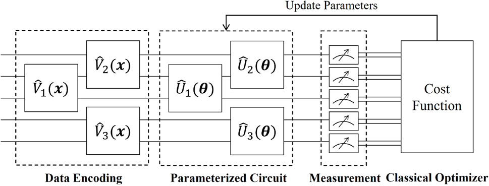
Figure 1. The frame of VQA.

VQA has the notable benefit of offering a general framework for solving diverse problems. In particular, hybrid quantum-classical machine learning models can be seen as quantum counterparts to extremely successful classical neural networks. Next, we will provide a detailed description of our RE-QCNN model based on VQA.

3 The structure of RE-QCNN

In Figure 2, the structure of the QCNN model is illustrated, which comprises three essential components: the quantum convolutional layer, the pooling layer, and the fully connected layer. This section provides a detailed description of our RE-QCNN model, starting from its fundamental components.

Figure 2

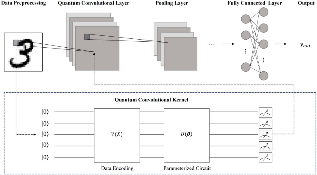
Figure 2. The structure of QCNN. The quantum convolutional layer contains several quantum convolutional kernels that transform the classical image into different feature maps. The detailed processing of classical data block into and out of the quantum convolutional kernel is provided within the dashed box.

3.1 Quantum convolutional layer

The classical convolutional layer is the pivotal layer in the classical CNN model. This layer performs convolutional operations on the classical image to extract features. Specifically, in the convolutional operation, a data block is obtained from the image using a sliding window, and a dot product is calculated between this data block and a weight matrix referred to as the classical convolutional kernel [29]. Unlike the classical convolutional layer, the main idea of a quantum convolutional layer is to extract features from the image by transforming the data block using a quantum convolutional kernel, also known as a quantum filter. The quantum filter consists of both a data encoding circuit and a parameterized quantum circuit.

Data encoding strategy. In our RE-QCNN model, amplitude encoding is adopted as the data encoding strategy. Let ${\{X_d\}}_{d=1}^D$ represent the preprocessed D data blocks extracted from the given classical image using a $\sqrt{N}\times \sqrt{N}$ sliding window with a stride of 1, which contain all the information of the image. Through the amplitude encoding strategy, each $X_d\in {\mathbb{R}}^N$ is encoded onto its respective quantum state denoted as |X_d⟩. Specifically,

$X_d\to |X_d\rangle =\frac{1}{‖X_d‖}{\displaystyle \sum _{i=1}^N}{X}_{di}|i\rangle ,(1)$

where X_di represents the i-th component of X_d and $‖X_d‖=\sqrt{{\sum }_{i=1}^N{X}_{di}^2}$ is the 2-norm of X_d. The N-dimensional vector X_d is encoded onto a superposition state |X_d⟩ with log  N qubits. As a result, amplitude encoding efficiently reduces the number of qubits within our model. However, its implementation is challenging. Specifically, to prepare an arbitrary quantum state, it is necessary to use a quantum circuit whose size scales exponentially with the number of qubits [38,39]. Nevertheless, when dealing with sparse datasets such as the MNIST dataset employed in our numerical experiments, amplitude encoding can be regarded as an efficient strategy. As mentioned in Refs. [50,51], the preparation of an arbitrary sparse quantum state can be accomplished using a quantum circuit whose size scales polynomially with the sparsity and the number of qubits.

Parameterized quantum circuit. We construct the parameterized quantum circuit based on the QAOA circuit that was originally designed to provide approximations for combinatorial optimization problems. The QAOA circuit starts by constructing two Hamiltonians H_B and H_C. Specifically, the Hamiltonian H_B is given by

$H_B={\displaystyle \sum _{q=1}^{\log N}}{\sigma }_q^x,(2)$

where ${\sigma }_q^x$ is the Pauli X operator acting on the q-th qubit. The Hamiltonian H_C is defined as

$H_C={\displaystyle \sum _{q=1}^{\log N-1}}\frac{1}{2}\left(I-{\sigma }_q^z{\sigma }_{q+1}^z\right),(3)$

where ${\sigma }_q^z$ is the Pauli Z operator acting on the q-th qubit. Subsequently, the p-layer QAOA circuit is constructed by iteratively applying $e^{-i{\beta }_j{H}_B}$ and $e^{-i{\gamma }_j{H}_C}$ for p rounds, given by

$U\left(\mathit{\beta },\mathit{\gamma }\right)={\displaystyle \prod _{j=1}^p}{e}^{-i{\beta }_j{H}_B}{e}^{-i{\gamma }_j{H}_C},(4)$

where parameter vectors β = [β₁, …, β_p], and γ = [γ₁, …, γ_p]. Figure 3A displays the structure of the QAOA circuit. In more detail, $e^{-i{\beta }_j{H}_B}$ and $e^{-i{\gamma }_j{H}_C}$ can be decomposed into single-qubit and two-qubit gates, as illustrated in Figures 3B, C. Specifically,

$e^{-i{\beta }_j{H}_B}={\displaystyle \prod _{q=1}^{\log N}}{R}_x{\left(2{\beta }_j\right)}_q,(5)$

$e^{-i{\gamma }_j{H}_C}={\displaystyle \prod _{q=1}^{\log N-1}}{e}^{-i\frac{{\gamma }_j}{2}I}{\mathrm{C}\mathrm{N}\mathrm{O}\mathrm{T}}_{\left(q,q+1\right)}{R}_z{\left(-{\gamma }_j\right)}_{q+1}{\mathrm{C}\mathrm{N}\mathrm{O}\mathrm{T}}_{\left(q,q+1\right)},(6)$

where R_x (⋅)_q represents Pauli X rotation operator acting on the q-th qubit, and R_z (⋅)_q denotes the Pauli Z rotation operator acting on the q-th qubit. An important characteristic of the QAOA circuit is parameter sharing, which refers to the sharing of the parameter among quantum gates within the same layer. This characteristic of the QAOA circuit reduces the required parameters for constructing the quantum convolutional layer. Moreover, the presence of two-qubit gates in the QAOA circuit provides it with a strong entanglement capability, resulting in a high expressibility of the quantum convolutional layer [48].

Figure 3

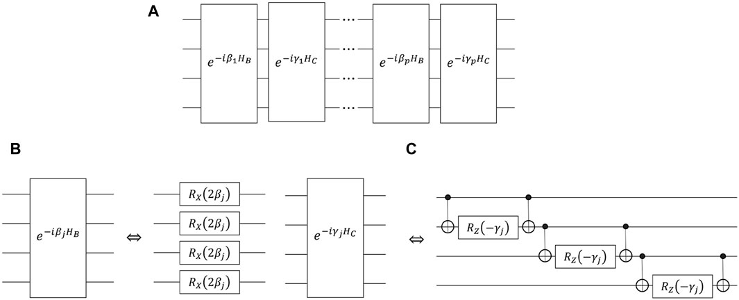
Figure 3. The structure of QAOA circuit.

Now, the output X_qcl (β, γ) of the quantum convolutional layer is a $\sqrt{D}\times \sqrt{D}$ matrix, given by

$X_{\mathit{qcl}}\left(\mathit{\beta },\mathit{\gamma }\right)=\left[\begin{array}{ccc}\hfill h_1\left(\mathit{\beta },\mathit{\gamma }\right)\hfill & \hfill \dots \hfill & \hfill h_{\sqrt{D}}\left(\mathit{\beta },\mathit{\gamma }\right)\hfill \\ \hfill ⋮\hfill & \hfill \dots \hfill & \hfill ⋮\hfill \\ \hfill h_{\left(\sqrt{D}-1\right)\sqrt{D}+1}\left(\mathit{\beta },\mathit{\gamma }\right)\hfill & \hfill \dots \hfill & \hfill h_D\left(\mathit{\beta },\mathit{\gamma }\right)\hfill \end{array}\right].(7)$

Here, for d ∈ {1, …, D}, h_d (β, γ) denotes the expectation value of a specific observable H, given by

$h_d\left(\mathit{\beta },\mathit{\gamma }\right)=⟨X_d|U^{†}\left(\mathit{\beta },\mathit{\gamma }\right)HU\left(\mathit{\beta },\mathit{\gamma }\right)|X_d⟩.(8)$

A common form of H is expressed as

$H={\displaystyle \sum _{s=1}^S}{c}_s{P}_s,(9)$

where $c_s\in \mathbb{R}$, and $P_s\in {\{I,{\sigma }^x,{\sigma }^y,{\sigma }^z\}}^{\otimes \log N}$. Specifically, we can use $H={\sum }_{s=1}^{\log N}{\sigma }_s^x$, where ${\sigma }_s^x$ represents the Pauli X operator acting on the s-th qubit.

3.2 Pooling layer and fully connected layer

Pooling layer. We employ a downsampling function denoted as down (⋅) to reduce the dimension of X_qcl (β, γ), and the resulting output X_pl (β, γ) is represented as

$X_{pl}\left(\mathit{\beta },\mathit{\gamma }\right)=\mathrm{d}\mathrm{o}\mathrm{w}\mathrm{n}\left(a\left(X_{\mathit{qcl}}\left(\mathit{\beta },\mathit{\gamma }\right)\right)\right),(10)$

where a (⋅) represents an activation function, such as the ReLU activation function. Here, down (⋅) is implemented by computing the maximum of different blocks of a (X_qcl (β, γ)). Specifically, these blocks can be obtained by applying a 2 × 2 sliding window with a stride of 2 to a (X_qcl (β, γ)), leading to the dimension of a (X_qcl (β, γ)) being reduced from $\sqrt{D}\times \sqrt{D}$ to $\sqrt{D}/2\times \sqrt{D}/2$.

Fully connected layer. The fully connected layer maps the features extracted by the quantum convolutional layer and the pooling layer to the m-dimensional label space. Specifically, the output y_out (β, γ, W, b) of the fully connected layer can be represented as

$y_{\mathit{out}}\left(\mathit{\beta },\mathit{\gamma },\mathit{W},\mathit{b}\right)=g\left({\mathit{W}}^T{X}_{pl}\left(\mathit{\beta },\mathit{\gamma }\right)+\mathit{b}\right),(11)$

where W denotes the D/4 × m weight matrix, X_pl (β, γ) is flattened into a D/4-dimensional vector, b represents the m-dimensional bias vector, and g (⋅) is an activation function, such as the softmax activation function used for the multi-class classification task.

3.3 Parameter updating

As described in Section 3.1 and 3.2, the forward propagation flow of our RE-QCNN model involves several mappings. Let ${\{X_d\}}_{d=1}^D$ be the preprocessed D data blocks. We denote the mapping of the quantum convolutional layer as $f_{\mathit{qcl}}:{\{X_d\}}_{d=1}^D\to X_{\mathit{qcl}}(\mathit{\beta },\mathit{\gamma })$, the mapping of the pooling layer as f_pl: X_qcl (β, γ) → X_pl (β, γ), the mapping of the fully connected layer as f_fcl: X_pl (β, γ) → y_out (β, γ, W, b), and the mapping of the cost function as l: y_out (β, γ, W, b) → C (β, γ, W, b). Now, the forward propagation flow is given by

$l◦f_{\mathit{fcl}}◦f_{pl}◦f_{\mathit{qcl}}.(12)$

Here, we focus on the parameter updates of β = [β₁, …, β_p] and γ = [γ₁, …, γ_p] in the quantum convolutional layer. Following the principles of backpropagation, for j ∈ {1, …, p}, the derivative of C (β, γ, W, b) with respect to γ_j is given by

$\begin{array}{cc}\hfill \frac{\partial C\left(\mathit{\beta },\mathit{\gamma },\mathit{W},\mathit{b}\right)}{\partial {\gamma }_j}& =\frac{\partial C\left(\mathit{\beta },\mathit{\gamma },\mathit{W},\mathit{b}\right)}{\partial y_{\mathit{out}}\left(\mathit{\beta },\mathit{\gamma },\mathit{W},\mathit{b}\right)}\cdot \frac{\partial y_{\mathit{out}}\left(\mathit{\beta },\mathit{\gamma },\mathit{W},\mathit{b}\right)}{\partial X_{pl}\left(\mathit{\beta },\mathit{\gamma }\right)}\cdot \frac{\partial X_{pl}\left(\mathit{\beta },\mathit{\gamma }\right)}{\partial X_{\mathit{qcl}}\left(\mathit{\beta },\mathit{\gamma }\right)}\cdot \frac{\partial X_{\mathit{qcl}}\left(\mathit{\beta },\mathit{\gamma }\right)}{\partial {\gamma }_j}\hfill \\ \hfill & ={\displaystyle \sum _{d=1}^D}\frac{\partial C\left(\mathit{\beta },\mathit{\gamma },\mathit{W},\mathit{b}\right)}{\partial y_{\mathit{out}}\left(\mathit{\beta },\mathit{\gamma },\mathit{W},\mathit{b}\right)}\cdot \frac{\partial y_{\mathit{out}}\left(\mathit{\beta },\mathit{\gamma },\mathit{W},\mathit{b}\right)}{\partial X_{pl}\left(\mathit{\beta },\mathit{\gamma }\right)}\cdot \frac{\partial X_{pl}\left(\mathit{\beta },\mathit{\gamma }\right)}{\partial h_d\left(\mathit{\beta },\mathit{\gamma }\right)}\cdot \frac{\partial h_d\left(\mathit{\beta },\mathit{\gamma }\right)}{\partial {\gamma }_j}.\hfill \end{array}(13)$

The first term relies on the specific form of the cost function. Specifically, the cost function quantifies the difference between the predicted labels of our model and the true labels. Different tasks typically use different cost functions. For instance, in the case of a multi-class classification task, cross-entropy is commonly employed as the cost function. Additionally, the second and third terms are associated with the mappings of the fully connected layer and the pooling layer, respectively. These three terms retain classical structures and can be calculated using traditional classical methods. Now, we focus on the calculation of the fourth term. It is crucial to note that the QAOA circuit exhibits parameter sharing, meaning that the same parameter is shared among quantum gates within the same layer. Considering this characteristic, we present the analytical expression for the derivative ∂h_d (β, γ)/∂γ_j.

Taking the 3-qubit QAOA circuit shown in Figure 4 as an example, we divide this QAOA circuit into five components: V₁, U₁ (−γ_j), V₂, U₂ (−γ_j), and V₃. Let ${\mathcal{V}}_1$, ${\mathcal{U}}_1(-{\gamma }_j)$, ${\mathcal{V}}_2$, ${\mathcal{U}}_2(-{\gamma }_j)$, and ${\mathcal{V}}_3$ denote the unitary channels corresponding to each component, respectively. Then, the expectation value h_d (β, γ) described by Eq. 8 can be reformulated as

$h_d\left(\mathit{\beta },\mathit{\gamma }\right)=\mathrm{t}\mathrm{r}\left[{\mathcal{V}}_1◦{\mathcal{U}}_1\left(-{\gamma }_j\right)◦{\mathcal{V}}_2◦{\mathcal{U}}_2\left(-{\gamma }_j\right)◦{\mathcal{V}}_3\left({\rho }_d\right)H\right],(14)$

where ρ_d = |X_d⟩⟨X_d|. Then, we have

$\begin{array}{cc}\hfill \frac{\partial h_d\left(\mathit{\beta },\mathit{\gamma }\right)}{\partial {\gamma }_j}& =\frac{\partial \mathrm{t}\mathrm{r}\left[{\mathcal{V}}_1◦{\mathcal{U}}_1\left(-{\gamma }_j\right)◦{\mathcal{V}}_2◦{\mathcal{U}}_2\left(-{\gamma }_j\right)◦{\mathcal{V}}_3\left({\rho }_d\right)H\right]}{\partial {\gamma }_j}\hfill \\ \hfill & =\mathrm{t}\mathrm{r}\left[{\mathcal{V}}_1◦\frac{\partial {\mathcal{U}}_1\left(-{\gamma }_j\right)}{\partial {\gamma }_j}◦{\mathcal{V}}_2◦{\mathcal{U}}_2\left(-{\gamma }_j\right)◦{\mathcal{V}}_3\left({\rho }_d\right)H\right]\hfill \\ \hfill & +\mathrm{t}\mathrm{r}\left[{\mathcal{V}}_1◦{\mathcal{U}}_1\left(-{\gamma }_j\right)◦{\mathcal{V}}_2◦\frac{\partial {\mathcal{U}}_2\left(-{\gamma }_j\right)}{\partial {\gamma }_j}◦{\mathcal{V}}_3\left({\rho }_d\right)H\right].\hfill \end{array}(15)$

Figure 4

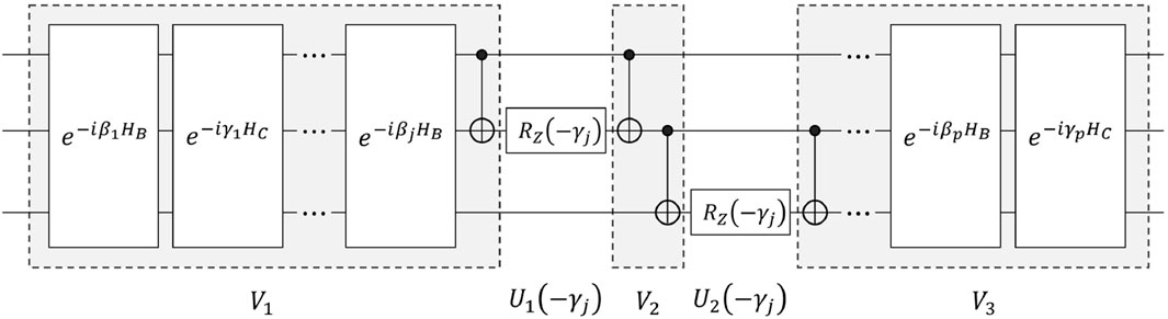
Figure 4. The illustration of QAOA circuit division.

Based on the parameter shift rule (see Supplementary Material), for i ∈ {1, 2}, each Pauli Z rotation channel ${\mathcal{U}}_i(-{\gamma }_j)$ satisfies

$\frac{\partial {\mathcal{U}}_i\left(-{\gamma }_j\right)}{\partial {\gamma }_j}=\frac{{\mathcal{U}}_i\left(-{\gamma }_j+\frac{\pi }{2}\right)-{\mathcal{U}}_i\left(-{\gamma }_j-\frac{\pi }{2}\right)}{2}.(16)$

Then, we have

$\begin{array}{cc}\hfill \frac{\partial h_d\left(\mathit{\beta },\mathit{\gamma }\right)}{\partial {\gamma }_j}& =\mathrm{t}\mathrm{r}\left[{\mathcal{V}}_1◦\frac{{\mathcal{U}}_1\left(-{\gamma }_j+\frac{\pi }{2}\right)-{\mathcal{U}}_1\left(-{\gamma }_j-\frac{\pi }{2}\right)}{2}◦{\mathcal{V}}_2◦{\mathcal{U}}_2\left(-{\gamma }_j\right)◦{\mathcal{V}}_3\left({\rho }_d\right)H\right]\hfill \\ \hfill & +\mathrm{t}\mathrm{r}\left[{\mathcal{V}}_1◦{\mathcal{U}}_1\left(-{\gamma }_j\right)◦{\mathcal{V}}_2◦\frac{{\mathcal{U}}_2\left(-{\gamma }_j+\frac{\pi }{2}\right)-{\mathcal{U}}_2\left(-{\gamma }_j-\frac{\pi }{2}\right)}{2}◦{\mathcal{V}}_3\left({\rho }_d\right)H\right]\hfill \\ \hfill & =\frac{1}{2}\mathrm{t}\mathrm{r}\left[{\mathcal{V}}_1◦{\mathcal{U}}_1\left(-{\gamma }_j+\frac{\pi }{2}\right)◦{\mathcal{V}}_2◦{\mathcal{U}}_2\left(-{\gamma }_j\right)◦{\mathcal{V}}_3\left({\rho }_d\right)H\right]\hfill \\ \hfill & -\frac{1}{2}\mathrm{t}\mathrm{r}\left[{\mathcal{V}}_1◦{\mathcal{U}}_1\left(-{\gamma }_j-\frac{\pi }{2}\right)◦{\mathcal{V}}_2◦{\mathcal{U}}_2\left(-{\gamma }_j\right)◦{\mathcal{V}}_3\left({\rho }_d\right)H\right]\hfill \\ \hfill & +\frac{1}{2}\mathrm{t}\mathrm{r}\left[{\mathcal{V}}_1◦{\mathcal{U}}_1\left(-{\gamma }_j\right)◦{\mathcal{V}}_2◦{\mathcal{U}}_2\left(-{\gamma }_j+\frac{\pi }{2}\right)◦{\mathcal{V}}_3\left({\rho }_d\right)H\right]\hfill \\ \hfill & -\frac{1}{2}\mathrm{t}\mathrm{r}\left[{\mathcal{V}}_1◦{\mathcal{U}}_1\left(-{\gamma }_j\right)◦{\mathcal{V}}_2◦{\mathcal{U}}_2\left(-{\gamma }_j-\frac{\pi }{2}\right)◦{\mathcal{V}}_3\left({\rho }_d\right)H\right].\hfill \end{array}(17)$

Indeed, by estimating the aforementioned four expectation values, we can obtain this derivative. The described process can naturally be extended to the QAOA circuit with log  N qubits. Similarly, we can obtain ∂C (β, γ, W, b)/∂β_j. Subsequently, by utilizing a gradient-based optimization method, we can update the parameters β and γ in the quantum convolutional layer.

3.4 Complexity analysis

In this section, we provide a detailed analysis of the complexity associated with the forward and backward propagation processes in the quantum convolutional layer.

For the forward propagation process, the D data blocks ${\{X_d\}}_{d=1}^D$ are extracted from the given classical image using a $\sqrt{N}\times \sqrt{N}$ sliding window with a stride of 1, which contain all the information of the image. Subsequently, ${\{X_d\}}_{d=1}^D$ are sequentially processed by the quantum convolutional kernel, and the resulting D expectation values ${\{h_d(\mathit{\beta },\mathit{\gamma })\}}_{d=1}^D$ as described in Eq. 8 form the output of the quantum convolutional layer, represented as a $\sqrt{D}\times \sqrt{D}$ matrix. In detail, the quantum convolutional kernel consists of the data encoding circuit and the parameterized quantum circuit. On one hand, the data encoding circuit adopts the amplitude encoding strategy as described in Eq. 1, and each $X_d\in {\mathbb{R}}^N$ is encoded onto its corresponding quantum state |X_d⟩ using log  N qubits. Notably, as stated in Theorem 1 of Ref. [50], when X_d is k-sparse (with k nonzero entries), the amplitude encoding strategy is achieved by a data encoding circuit of size $\mathcal{O}(k\log N)$, which includes $\mathcal{O}(k\log k+\log N)$ single-qubit gates and $\mathcal{O}(k\log N)$ CNOT gates. Additionally, a quantum superposition query is required to obtain the k nonzero entries of X_d [52]. On the other hand, the parameterized quantum circuit is constructed based on the QAOA circuit U (β, γ) with log  N qubits, as described in Eq. 4. According to Eq.5 and 6, $e^{-i{\beta }_j{H}_B}$ can be decomposed into log  N single-qubit gates, while $e^{-i{\beta }_j{H}_C}$ can be decomposed into log  N single-qubit gates and 2 log  N CNOT gates in each layer of the QAOA circuit. Therefore, the total number of quantum gates required to implement U (β, γ) is $\mathcal{O}(p\mathrm{p}\mathrm{o}\mathrm{l}\mathrm{y}(\log N))$, where p is the number of layers. Finally, by performing measurements, we estimate each h_d (β, γ) with a complexity of $\mathcal{O}((k+p)\mathrm{p}\mathrm{o}\mathrm{l}\mathrm{y}(\log N)/{ϵ}^2)$, where ϵ represents the additive error in estimating this expectation value. Therefore, the overall complexity of the forward propagation process in the quantum convolutional layer is $\mathcal{O}(D(k+p)\mathrm{p}\mathrm{o}\mathrm{l}\mathrm{y}(\log N)/{ϵ}^2)$.

For the backward propagation process, the complexity of the quantum convolutional layer primarily arises from the estimation of ${\{{\{\frac{\partial h_d(\mathit{\beta },\mathit{\gamma })}{\partial {\gamma }_j}\}}_{j=1}^p\}}_{d=1}^D$ and ${\{{\{\frac{\partial h_d(\mathit{\beta },\mathit{\gamma })}{\partial {\beta }_j}\}}_{j=1}^p\}}_{d=1}^D$. As each $\frac{\partial h_d(\mathit{\beta },\mathit{\gamma })}{\partial {\gamma }_j}$ and $\frac{\partial h_d(\mathit{\beta },\mathit{\gamma })}{\partial {\beta }_j}$ can be obtained according to Eq. 17, the overall complexity of the backward propagation process in the quantum convolutional layer is $\mathcal{O}(Dp(k+p)\mathrm{p}\mathrm{o}\mathrm{l}\mathrm{y}(\log N)/{ϵ}^2)$.

Increasing the number of layers p in the parameterized quantum circuit enhances its expressibility, thereby improving the numerical performance of our model. However, when the parameterized quantum circuit reaches a specific number of layers, it may exhibit the barren plateau phenomenon [53,54]. This phenomenon poses challenges to the model training and impacts its numerical performance. Taking these factors into account, choosing p to be $\mathcal{O}(\log N)$ is reasonable. In addition, the additive error ϵ is considered to be a constant, which is a general choice in the context of quantum machine learning [55]. In this context, the complexity of both the forward and backward propagation processes is $\mathcal{O}(Dk\mathrm{p}\mathrm{o}\mathrm{l}\mathrm{y}(\log N))$. Now, we can conclude that the complexity of the quantum convolutional layer is $\mathcal{O}(Dk\mathrm{p}\mathrm{o}\mathrm{l}\mathrm{y}(\log N))$.

Meanwhile, for the forward propagation process of the classical convolutional layer, the aforementioned D data blocks ${\{X_d\}}_{d=1}^D$, which are all k-sparse N-dimensional vectors, are sequentially processed by the classical convolutional kernel. This results in D feature values ${\{h_d(\mathit{w})\}}_{d=1}^D$. Specifically, each h_d(w) is given by h_d(w) = w^TX_d, where w is the N-dimensional weight vector [29]. Considering that each X_d is k-sparse, the calculation of each h_d(w) has a complexity of $\mathcal{O}(k)$. Additionally, N classical queries are required to obtain the k nonzero entries of X_d. Therefore, the overall complexity of the forward propagation process in the classical convolutional layer is $\mathcal{O}(Dk)$ [47]. For the backward propagation process, the complexity of the classical convolutional layer primarily arises from the calculation of ${\{{\{\frac{\partial h_d(\mathit{w})}{\partial w_j}\}}_{j=1}^N\}}_{d=1}^D$. Since each $\frac{\partial h_d(\mathit{w})}{\partial w_j}$ is calculated with a complexity of $\mathcal{O}(k)$, the overall complexity of the backward propagation process is $\mathcal{O}(DNk)$. Now, we can conclude that the complexity of the classical convolutional layer is $\mathcal{O}(DNk)$.

The complexity analysis of the quantum and classical convolutional layers, respectively handling D k-sparse N-dimensional data blocks, is shown in Table 1. There is a trade-off between the sizes of D and N, that is D and N form an inverse proportional relationship. As a result, when N is relatively large and the sparsity k of the data block is $\mathcal{O}(\log N)$, the quantum convolutional layer demonstrates a significant reduction in computational resources compared to the classical CNN model.

Table 1

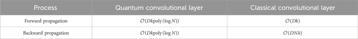
Table 1. Complexity analysis of the quantum (gate complexity) and classical (computational complexity) convolutional layers. Here, the quantum and classical convolutional layers handle D k-sparse N-dimensional data blocks respectively.

4 Numerical experiments

To evaluate the performance of our RE-QCNN model, we conduct numerical experiments on the MNIST and Fashion-MNIST datasets.

4.1 Performance of RE-QCNN on MNIST dataset

The MNIST dataset consists of a training set with 60,000 images and a test set with 10,000 images. Each image in this dataset is composed of 784 (28 × 28) pixels. The visualization of the MNIST dataset is depicted in Figure 5.

Figure 5

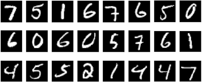
Figure 5. The visualization of MNIST dataset.

In detail, we conduct numerical experiments using the 2-layer RE-QCNN model, which includes two quantum convolutional layers and two pooling layers. The objective of these numerical experiments is to recognize handwritten digit images across all categories. The model configuration details can be found in Table 2. In this configuration, the first quantum convolutional layer consists of a single quantum filter implemented using a 5-qubit QAOA circuit with two layers. Specifically, the quantum convolutional layer applies a 5 × 5 sliding window with a stride of 1 to the normalized 28 × 28 image matrix, resulting in 576 data blocks. Each data block, consisting of 25 pixels, is encoded onto its respective quantum state using 5 qubits through the amplitude encoding strategy. Subsequently, the 576 data-encoding quantum states are sequentially processed by the 2-layer QAOA circuit. Finally, the measurement outcomes of the observable $H={\sum }_{s=1}^5{\sigma }_s^x$ are obtained, resulting in 576 expectation values. These expectation values form the output of the first quantum convolutional layer, represented as a 24 × 24 matrix. The second quantum convolutional layer comprises 6 quantum filters, and each quantum filter is also implemented using a 5-qubit QAOA circuit with two layers. Before the output of each quantum convolutional layer enters the pooling layer, it is subjected to a ReLU activation function, followed by a downsampling function. Additionally, for this multi-class classification task, the fully connected layer with the softmax activation function generates the predicted label, and cross-entropy is employed as the cost function. We conduct cross-validation experiments using 2-fold, 3-fold, 5-fold, and 7-fold validation on a total of 70,000 images.

Table 2

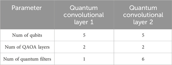
Table 2. The configuration of the 2-layer RE-QCNN on MNIST dataset.

For each cross-validation experiment, the Receiver Operating Characteristic (ROC) curve is depicted in Figure 6A. The ROC curves reveal that our model trained using 2-fold cross-validation lacks superior generalization capability. Specifically, at the False Positive Rate (FPR) of 2%, our model achieves the True Positive Rate (TPR) of 89%, indicating a convergence phase. Complete convergence is achieved at the FPR of 10%. In contrast, our model trained using 7-fold cross-validation demonstrates superior generalization capability. The ROC curve exhibits noticeable improvement at the FPR of 2%, and complete convergence is achieved at the FPR of 10%. Furthermore, the stability of our model is evaluated using the confusion matrix, as depicted in Figure 6B. Overall, our model attains high accuracy in recognizing handwritten digit images across all categories.

Figure 6

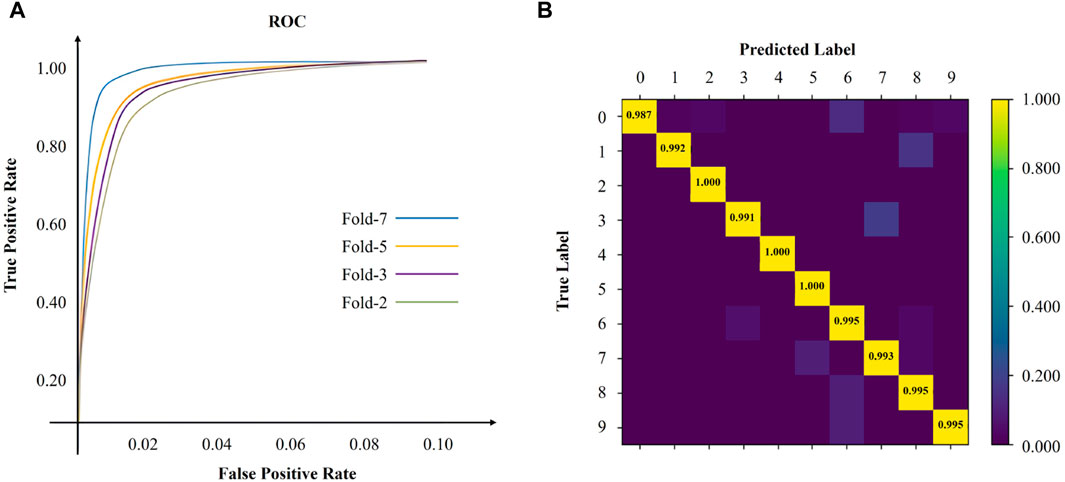
Figure 6. The performance of RE-QCNN on MNIST dataset.

4.2 Performance of RE-QCNN on Fashion-MNIST dataset

The Fashion-MNIST dataset consists of grayscale images of fashion products, where each image is composed of 28 × 28 pixels. This dataset comprises 70,000 images from 10 categories, with 7,000 images per category. The training set contains 60,000 images, while the test set contains 10,000 images. The Fashion-MNIST dataset is considered to be more complex compared to the conventional MNIST dataset. The visualization of the Fashion-MNIST dataset is depicted in Figure 7. In detail, we conduct numerical experiments to comprehensively assess our model’s performance on the Fashion-MNIST dataset. The objective of these numerical experiments is to recognize images across all categories using the 2-layer RE-QCNN model, which includes two quantum convolutional layers and two pooling layers. Next, we present the performance of our model as obtained from numerical experiments involving the QAOA circuit with different random initial parameters, various numbers of layers, and different levels of measurement errors.

Figure 7

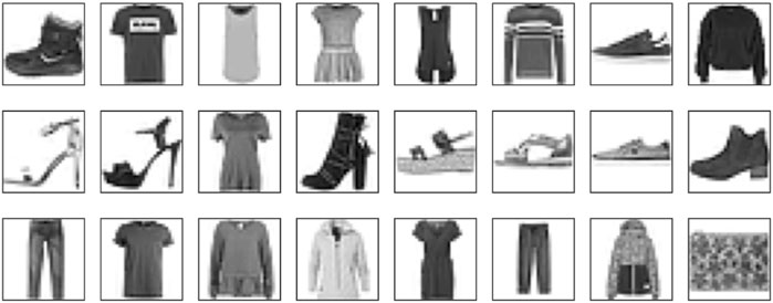
Figure 7. The visualization of Fashion-MNIST dataset.

Firstly, for the numerical experiments involving the QAOA circuit with five different sets of random initial parameters, the model configuration is consistent with the configuration used for the MNIST dataset, with some details being different. Specifically, the first quantum convolutional layer consists of 40 quantum filters. Each of these quantum filters is implemented using a 5-qubit QAOA circuit with four layers. The second quantum convolutional layer comprises 80 quantum filters, and each quantum filter is also implemented using a 5-qubit QAOA circuit with four layers. These differences can be found in Table 3. Additionally, since we are also dealing with a multi-class classification task, cross-entropy is employed as the cost function. The accuracy of our model, using the QAOA circuit with five different sets of random initial parameters, is depicted as a function of epoch in Figure 8A. This figure illustrates that the highest achieved accuracy is 92.94%, the lowest accuracy is 92.20%, and the average accuracy is 92.59%.

Table 3

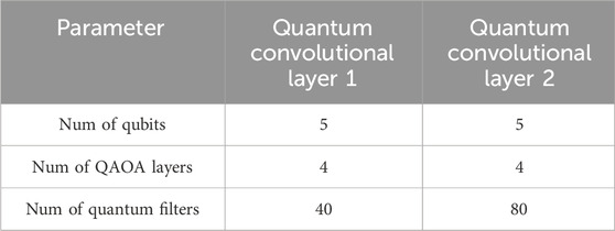
Table 3. The configuration of the 2-layer RE-QCNN on Fashion-MNIST dataset.

Figure 8

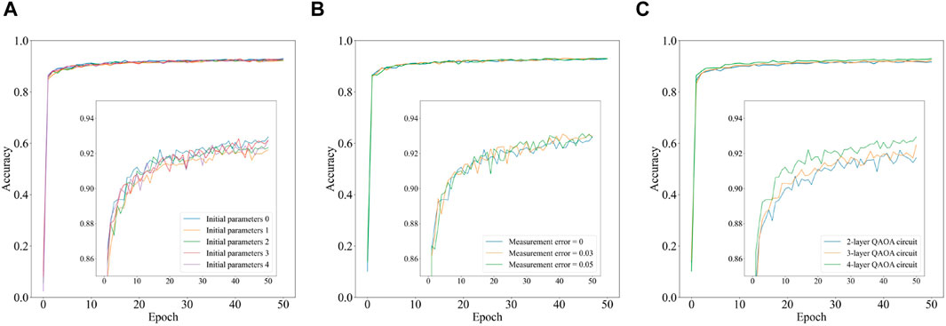
Figure 8. The performance of RE-QCNN on Fashion-MNIST dataset.

Subsequently, using the same model configuration and the optimal initial parameters of the QAOA circuit mentioned above, we assess the performance of our model under measurement errors of 0, 0.03, and 0.05. Figure 8B reveals that the performance of our model is quite resilient to such errors. Considering that the number of layers in the parameterized quantum circuit of our model is relatively shallow, gate errors may be effectively mitigated by error mitigation techniques [56-59], which suggests small gate errors may not significantly affect the performance of our model. Therefore, we only assess the performance of our model under different levels of measurement errors.

Finally, using the same model configuration and the optimal initial parameters of the QAOA circuit mentioned above, we vary the number of layers in the QAOA circuit to 2, 3, and 4. The corresponding accuracy of our model is depicted as a function of epoch in Figure 8C. This figure demonstrates that our model achieves superior performance when a larger number of layers are employed in the QAOA circuit. The result aligns with the viewpoint that increasing the number of layers enhances the entanglement capability of the QAOA circuit.

Overall, our model exhibits excellent numerical performance on the more complex Fashion-MNIST dataset compared to the MNIST dataset.

5 Conclusion

To explore the potential quantum advantages of the QCNN model, it is common to compare the prediction accuracy directly between the quantum and classical models. However, according to the “no-free-lunch” conjecture, a specific QCNN or CNN model may not exhibit excellent numerical performance across all tasks. This perspective is highly dependent on the specific task and may be influenced by random factors. A more solid perspective for exploring the potential quantum advantages involves comparing computational resources by quantifying the number of fundamental computational elements used in the training and prediction processes. By considering both perspectives, a more comprehensive showcase of the potential quantum advantages can be achieved. In this paper, we propose a computationally resource-efficient QCNN model. Our model significantly reduces the computational resources required for the quantum convolutional layer compared to the classical CNN model. Additionally, our model achieves high accuracy in the multi-class classification tasks of recognizing images from the MNIST and Fashion-MNIST datasets. Our results hold significant importance in exploring the potential quantum advantages of the QCNN model in the NISQ era.

Several important aspects merit further investigation in the field of QCNN. Specifically, a crucial research topic is to explore the impact of parameterized quantum circuits on the numerical performance of the QCNN model. Additionally, it is worth considering the exploration of novel data encoding strategies, particularly those capable of handling high-dimensional data such as video streams and 3D medical images. This research will greatly contribute to diversifying the application scenarios of the QCNN model.

Data availability statement

The original contributions presented in the study are included in the article/Supplementary Material, further inquiries can be directed to the corresponding authors.

Author contributions

YS: Writing–original draft, Software, Visualization, Writing–review and editing, Conceptualization, Data curation, Formal Analysis, Investigation, Methodology, Validation. JL: Writing–original draft, Writing–review and editing, Investigation, Validation, Visualization. YW: Writing–review and editing, Software, Data curation, Supervision, Validation. SQ: Writing–review and editing, Funding acquisition, Supervision, Validation. QW: Writing–review and editing, Funding acquisition, Supervision, Validation. FG: Writing–review and editing, Funding acquisition, Supervision, Validation.

Funding

The author(s) declare that financial support was received for the research, authorship, and/or publication of this article. This work is supported by National Natural Science Foundation of China (Grant Nos. 62372048, 62371069, and 62272056), Beijing Natural Science Foundation (Grant No. 4222031), and China Scholarship Council (Grant No. 202006470011).

Acknowledgments

We would like to thank Yueran Hou, Jiashao Shen, Ximing Wang, and Shengyao Wu to provide helpful suggestions for the manuscript.

Conflict of interest

The authors declare that the research was conducted in the absence of any commercial or financial relationships that could be construed as a potential conflict of interest.

Publisher’s note

All claims expressed in this article are solely those of the authors and do not necessarily represent those of their affiliated organizations, or those of the publisher, the editors and the reviewers. Any product that may be evaluated in this article, or claim that may be made by its manufacturer, is not guaranteed or endorsed by the publisher.

Supplementary material

The Supplementary Material for this article can be found online at: https://www.frontiersin.org/articles/10.3389/fphy.2024.1362690/full#supplementary-material

References

1. Harrow AW, Montanaro A. Quantum computational supremacy. Nature (2017) 549:203–9. doi:10.1038/nature23458

PubMed Abstract | CrossRef Full Text | Google Scholar

2. Shor PW. Polynomial-time algorithms for prime factorization and discrete logarithms on a quantum computer. SIAM Rev (1999) 41:303–32. doi:10.1137/S0036144598347011

CrossRef Full Text | Google Scholar

3. Grover LK. Quantum mechanics helps in searching for a needle in a haystack. Phys Rev Lett (1997) 79:325–8. doi:10.1103/PhysRevLett.79.325

CrossRef Full Text | Google Scholar

4. Biamonte J, Wittek P, Pancotti N, Rebentrost P, Wiebe N, Lloyd S. Quantum machine learning. Nature (2017) 549:195–202. doi:10.1038/nature23474

PubMed Abstract | CrossRef Full Text | Google Scholar

5. Dunjko V, Briegel HJ. Machine learning and artificial intelligence in the quantum domain: a review of recent progress. Rep Prog Phys (2018) 81:074001. doi:10.1088/1361-6633/aab406

PubMed Abstract | CrossRef Full Text | Google Scholar

6. Schütt KT, Chmiela S, Von Lilienfeld OA, Tkatchenko A, Tsuda K, Müller K-R. Machine learning meets quantum physics. Lecture Notes Phys (2020). doi:10.1007/978-3-030-40245-7

CrossRef Full Text | Google Scholar

7. Harrow AW, Hassidim A, Lloyd S. Quantum algorithm for linear systems of equations. Phys Rev Lett (2009) 103:150502. doi:10.1103/PhysRevLett.103.150502

PubMed Abstract | CrossRef Full Text | Google Scholar

8. Rebentrost P, Steffens A, Marvian I, Lloyd S. Quantum singular-value decomposition of nonsparse low-rank matrices. Phys Rev A (2018) 97:012327. doi:10.1103/PhysRevA.97.012327

CrossRef Full Text | Google Scholar

9. Somma R, Childs A, Kothari R. Quantum linear systems algorithm with exponentially improved dependence on precision. APS March Meet Abstr (2016) 2016. doi:10.1137/16M1087072

CrossRef Full Text | Google Scholar

10. Wiebe N, Braun D, Lloyd S. Quantum algorithm for data fitting. Phys Rev Lett (2012) 109:050505. doi:10.1103/PhysRevLett.109.050505

PubMed Abstract | CrossRef Full Text | Google Scholar

11. Brandao FG, Svore KM. Quantum speed-ups for solving semidefinite programs. In: 2017 IEEE 58th Annual Symposium on Foundations of Computer Science (FOCS) (IEEE); 15-17 October 2017; Berkeley, California, USA (2017). p. 415–26. doi:10.1109/FOCS.2017.45

CrossRef Full Text | Google Scholar

12. Rebentrost P, Schuld M, Wossnig L, Petruccione F, Lloyd S. Quantum gradient descent and Newton’s method for constrained polynomial optimization. New J Phys (2019) 21:073023. doi:10.1088/1367-2630/ab2a9e

CrossRef Full Text | Google Scholar

13. Lloyd S, Mohseni M, Rebentrost P. Quantum principal component analysis. Nat Phys (2014) 10:631–3. doi:10.1038/nphys3029

CrossRef Full Text | Google Scholar

14. Rebentrost P, Mohseni M, Lloyd S. Quantum support vector machine for big data classification. Phys Rev Lett (2014) 113:130503. doi:10.1103/PhysRevLett.113.130503

PubMed Abstract | CrossRef Full Text | Google Scholar

15. Wei S, Chen Y, Zhou Z, Long G. A quantum convolutional neural network on nisq devices. AAPPS Bull (2022) 32:2–11. doi:10.1007/s43673-021-00030-3

CrossRef Full Text | Google Scholar

16. Preskill J. Quantum computing in the nisq era and beyond. Quantum (2018) 2:79. doi:10.22331/q-2018-08-06-79

CrossRef Full Text | Google Scholar

17. Farhi E, Neven H. Classification with quantum neural networks on near term processors (2018). arXiv preprint arXiv:1802.06002.

Google Scholar

18. Schuld M, Bocharov A, Svore KM, Wiebe N. Circuit-centric quantum classifiers. Phys Rev A (2020) 101:032308. doi:10.1103/PhysRevA.101.032308

CrossRef Full Text | Google Scholar

19. Li W, Lu Z-d., Deng D-L, Guo Y, Chen J, Shang S, et al. (2022). Quantum neural network classifiers: a tutorial. SciPost Phys Lecture Notes. 19, 61, doi:10.1186/s12985-022-01789-z

CrossRef Full Text | Google Scholar

20. Massoli FV, Vadicamo L, Amato G, Falchi F. A leap among quantum computing and quantum neural networks: a survey. ACM Comput Surv (2022) 55:1–37. doi:10.1145/3529756

CrossRef Full Text | Google Scholar

21. Song Y, Wu Y, Wu S, Li D, Wen Q, Qin S, et al. A quantum federated learning framework for classical clients (2023). arXiv preprint arXiv:2312.11672.

Google Scholar

22. McClean JR, Romero J, Babbush R, Aspuru-Guzik A. The theory of variational hybrid quantum-classical algorithms. New J Phys (2016) 18:023023. doi:10.1088/1367-2630/18/2/023023

CrossRef Full Text | Google Scholar

23. Cerezo M, Arrasmith A, Babbush R, Benjamin SC, Endo S, Fujii K, et al. Variational quantum algorithms. Nat Rev Phys (2021) 3:625–44. doi:10.1038/s42254-021-00348-9

CrossRef Full Text | Google Scholar

24. Bharti K, Cervera-Lierta A, Kyaw TH, Haug T, Alperin-Lea S, Anand A, et al. Noisy intermediate-scale quantum algorithms. Rev Mod Phys (2022) 94:015004. doi:10.1103/RevModPhys.94.015004

CrossRef Full Text | Google Scholar

25. Wu Y, Huang Z, Sun J, Yuan X, Wang JB, Lv D. Orbital expansion variational quantum eigensolver. Quan Sci Tech (2023) 8:045030. doi:10.1088/2058-9565/acf9c7

CrossRef Full Text | Google Scholar

26. Wu Y, Wu B, Wang J, Yuan X. Quantum phase recognition via quantum kernel methods. Quantum (2023) 7:981. doi:10.22331/q-2023-04-17-981

CrossRef Full Text | Google Scholar

27. Oh S, Choi J, Kim J. A tutorial on quantum convolutional neural networks (qcnn). In: 2020 International Conference on Information and Communication Technology Convergence (ICTC); October 21-23, 2020; Jeju Island, Korea (South) (2020). p. 236–9. doi:10.1109/ICTC49870.2020.9289439

CrossRef Full Text | Google Scholar

28. Li Z, Liu F, Yang W, Peng S, Zhou J. A survey of convolutional neural networks: analysis, applications, and prospects. IEEE Trans Neural Networks Learn Syst (2022) 33:6999–7019. doi:10.1109/TNNLS.2021.3084827

PubMed Abstract | CrossRef Full Text | Google Scholar

29. Gu J, Wang Z, Kuen J, Ma L, Shahroudy A, Shuai B, et al. Recent advances in convolutional neural networks. Pattern recognition (2018) 77:354–77. doi:10.1016/j.patcog.2017.10.013

CrossRef Full Text | Google Scholar

30. Cong I, Choi S, Lukin MD. Quantum convolutional neural networks. Nat Phys (2019) 15:1273–8. doi:10.1038/s41567-019-0648-8

CrossRef Full Text | Google Scholar

31. Liu J, Lim KH, Wood KL, Huang W, Guo C, Huang H-L. Hybrid quantum-classical convolutional neural networks. Sci China Phys Mech Astron (2021) 64:290311. doi:10.1007/s11433-021-1734-3

CrossRef Full Text | Google Scholar

32. Houssein EH, Abohashima Z, Elhoseny M, Mohamed WM. Hybrid quantum-classical convolutional neural network model for covid-19 prediction using chest x-ray images. J Comput Des Eng (2022) 9:343–63. doi:10.1093/jcde/qwac003

CrossRef Full Text | Google Scholar

33. Bokhan D, Mastiukova AS, Boev AS, Trubnikov DN, Fedorov AK. Multiclass classification using quantum convolutional neural networks with hybrid quantum-classical learning. Front Phys (2022) 10. doi:10.3389/fphy.2022.1069985

CrossRef Full Text | Google Scholar

34. Matic A, Monnet M, Lorenz JM, Schachtner B, Messerer T. Quantum-classical convolutional neural networks in radiological image classification. In: 2022 IEEE International Conference on Quantum Computing and Engineering (QCE) (IEEE); 18-23 September 2022; Broomfield, Colorado, USA (2022). p. 56. –66. doi:10.1109/QCE53715.2022.00024

CrossRef Full Text | Google Scholar

35. Henderson M, Shakya S, Pradhan S, Cook T. Quanvolutional neural networks: powering image recognition with quantum circuits. Quan Machine Intelligence (2020) 2:2. doi:10.1007/s42484-020-00012-y

CrossRef Full Text | Google Scholar

36. Chen SY-C, Wei T-C, Zhang C, Yu H, Yoo S. Quantum convolutional neural networks for high energy physics data analysis. Phys Rev Res (2022) 4:013231. doi:10.1103/PhysRevResearch.4.013231

CrossRef Full Text | Google Scholar

37. Amin J, Sharif M, Gul N, Kadry S, Chakraborty C. Quantum machine learning architecture for covid-19 classification based on synthetic data generation using conditional adversarial neural network. Cogn Comput (2022) 14:1677–88. doi:10.1007/s12559-021-09926-6

CrossRef Full Text | Google Scholar

38. Mottonen M, Vartiainen JJ, Bergholm V, Salomaa MM. Transformation of quantum states using uniformly controlled rotations (2004). arXiv preprint quant-ph/0407010.

Google Scholar

39. Iten R, Colbeck R, Kukuljan I, Home J, Christandl M. Quantum circuits for isometries. Phys Rev A (2016) 93:032318. doi:10.1103/PhysRevA.93.032318

CrossRef Full Text | Google Scholar

40. Farhi E, Goldstone J, Gutmann S. A quantum approximate optimization algorithm (2014). arXiv preprint arXiv:1411.4028.

Google Scholar

41. Hadfield S, Wang Z, O’gorman B, Rieffel EG, Venturelli D, Biswas R. From the quantum approximate optimization algorithm to a quantum alternating operator ansatz. Algorithms (2019) 12:34. doi:10.3390/a12020034

CrossRef Full Text | Google Scholar

42. Song Y, Wu Y, Qin S, Wen Q, Wang JB, Gao F. Trainability analysis of quantum optimization algorithms from a bayesian lens (2023). arXiv preprint arXiv:2310.06270.

Google Scholar

43. Liu T, Fang S, Zhao Y, Wang P, Zhang J. Implementation of training convolutional neural networks (2015). arXiv preprint arXiv:1506.01195.

Google Scholar

44. Romero J, Babbush R, McClean JR, Hempel C, Love PJ, Aspuru-Guzik A. Strategies for quantum computing molecular energies using the unitary coupled cluster ansatz. Quan Sci Tech (2018) 4:014008. doi:10.1088/2058-9565/aad3e4

CrossRef Full Text | Google Scholar

45. Mitarai K, Negoro M, Kitagawa M, Fujii K. Quantum circuit learning. Phys Rev A (2018) 98:032309. doi:10.1103/PhysRevA.98.032309

CrossRef Full Text | Google Scholar

46. Schuld M, Bergholm V, Gogolin C, Izaac J, Killoran N. Evaluating analytic gradients on quantum hardware. Phys Rev A (2019) 99:032331. doi:10.1103/PhysRevA.99.032331

CrossRef Full Text | Google Scholar

47. Kiranyaz S, Avci O, Abdeljaber O, Ince T, Gabbouj M, Inman DJ. 1d convolutional neural networks and applications: a survey. Mech Syst signal Process (2021) 151:107398. doi:10.1016/j.ymssp.2020.107398

CrossRef Full Text | Google Scholar

48. Sim S, Johnson PD, Aspuru-Guzik A. Expressibility and entangling capability of parameterized quantum circuits for hybrid quantum-classical algorithms. Adv Quan Tech (2019) 2:1900070. doi:10.1002/qute.201900070

CrossRef Full Text | Google Scholar

49. Kingma DP, Ba J. Adam: a method for stochastic optimization (2014). arXiv preprint arXiv:1412.6980.

Google Scholar

50. Gleinig N, Hoefler T. An efficient algorithm for sparse quantum state preparation. In: 2021 58th ACM/IEEE Design Automation Conference (DAC) (IEEE); December 5 - 9, 2021; San Francisco, CA, USA (2021). p. 433–8.

CrossRef Full Text | Google Scholar

51. Malvetti E, Iten R, Colbeck R. Quantum circuits for sparse isometries. Quantum (2021) 5:412. doi:10.22331/q-2021-03-15-412

CrossRef Full Text | Google Scholar

52. Camps D, Lin L, Van Beeumen R, Yang C. Explicit quantum circuits for block encodings of certain sparse matrices (2022). arXiv preprint arXiv:2203.10236.

PubMed Abstract | Google Scholar

53. McClean JR, Boixo S, Smelyanskiy VN, Babbush R, Neven H. Barren plateaus in quantum neural network training landscapes. Nat Commun (2018) 9:4812–6. doi:10.1038/s41467-018-07090-4

PubMed Abstract | CrossRef Full Text | Google Scholar

54. Cerezo M, Sone A, Volkoff T, Cincio L, Coles PJ. Cost function dependent barren plateaus in shallow parametrized quantum circuits. Nat Commun (2021) 12:1791. doi:10.1038/s41467-021-21728-w

PubMed Abstract | CrossRef Full Text | Google Scholar

55. Huang H-Y, Broughton M, Cotler J, Chen S, Li J, Mohseni M, et al. Quantum advantage in learning from experiments. Science (2022) 376:1182–6. doi:10.1126/science.abn7293

PubMed Abstract | CrossRef Full Text | Google Scholar

56. Endo S, Cai Z, Benjamin SC, Yuan X. Hybrid quantum-classical algorithms and quantum error mitigation. J Phys Soc Jpn (2021) 90:032001. doi:10.7566/jpsj.90.032001

CrossRef Full Text | Google Scholar

57. Cai Z, Babbush R, Benjamin SC, Endo S, Huggins WJ, Li Y, et al. Quantum error mitigation. Rev Mod Phys (2023) 95:045005. doi:10.1103/revmodphys.95.045005

CrossRef Full Text | Google Scholar

58. Endo S, Benjamin SC, Li Y. Practical quantum error mitigation for near-future applications. Phys Rev X (2018) 8:031027. doi:10.1103/physrevx.8.031027

CrossRef Full Text | Google Scholar

59. Temme K, Bravyi S, Gambetta JM. Error mitigation for short-depth quantum circuits. Phys Rev Lett (2017) 119:180509. doi:10.1103/physrevlett.119.180509

PubMed Abstract | CrossRef Full Text | Google Scholar