Research on fishing vessel recognition based on vessel behavior characteristics from AIS data

The Automatic Identification System (AIS) is one of the most important navigation assistance systems and plays a pivotal role in vessel monitoring. However, some fishing vessels disguise themselves as other vessel types during fishing bans to engage in illegal fishing activities, causing significant damage to marine ecosystem. To address this challenge and accurately identify vessel types, a BP-AdaBoost classification algorithm is developed by integrating backpropagation (BP) neural networks with ensemble learning techniques. The proposed algorithm leverages the AdaBoost method to combine multiple BP neural network weak classifiers into a strong classifier, effectively mitigating the slow convergence rate and susceptibility to local optima inherent in BP neural networks. By configuring the output nodes of the BP neural network to match the number of target classes, the AdaBoost algorithm achieves robust multi-class classification functionality. Historical AIS data are analyzed to extract static features, vessel behavior features, and temporal features for vessel classification. To minimize model overfitting, the Maximal Information Coefficient algorithm is employed to assess feature importance, and optimal feature combinations are determined through systematic feature selection experiments. Experiments are conducted using AIS data from the Pearl River Estuary in China, targeting the classification of cargo ships, fishing vessel, tanker, and passenger ships. The performance of the proposed method is compared with other machine learning algorithms. The results demonstrated classification accuracies of 90.8% for cargo ships, 95.6% for fishing vessels, 97.5% for tankers, and 98% for passenger ships, with an overall classification accuracy of 95%. Additionally, the BP-AdaBoost algorithm exhibited superior performance across other classification evaluation metrics. Specifically, the proposed algorithm outperformed the BP neural network by 4.5% and the support vector machine by 12.6% in overall classification accuracy. These findings indicate that the BP-AdaBoost algorithm is capable of effectively identifying vessel types based on historical trajectory data, providing a solid foundation for combating illegal fishing, detecting abnormal vessels, and identifying irregular vessel behaviors.

1 Introduction

With the continuous increase in the number of fishing vessels and the advancement of fishing technologies, the intensity of fishing in coastal waters escalates, leading to significant marine ecological damage and a shortage of fishery resources (Pham et al., 2014). Against this backdrop, illegal fishing activities have a huge impact on marine ecological protection. China has makes significant efforts to restore coastal fishery resources and regulate fishing activities, the most important of which is the close monitoring of fishing vessels through the Automatic Identification System (AIS). AIS is a new navigation assistance system that the International Maritime Organization (IMO) mandates for all Class A vessels (Sheng and Yin, 2018), enabling identification, positioning, and collision avoidance among ships. It encompasses dynamic, static, navigational, and safety information. However, the information in AIS faces the challenge that the vessel types reported may not accurately reflect the true types of the vessels; some vessels intentionally conceal their true type when engaging in smuggling, illegal fishing, or other unlawful activities. If vessel types can be derived from historical AIS data, then the corresponding prior knowledge of a particular vessel type can be applied to maritime traffic management. Therefore, accurately identifying vessel types enhances the situational awareness of relevant authorities and holds significant value in areas such as maritime surveillance, disguise identification, vessel behavior pattern mining, and anomaly detection, especially in the fight against illegal fishing.

Although high-resolution remote sensing images can provide rich detail, they also present challenges such as high computational demands and long processing times. Additionally, image compression may lead to data loss, which can affect the accuracy of vessel classification. In contrast, AIS data has clear advantages. AIS data is transmitted in real-time through shore-based or satellite communication networks, allowing global users to access trajectory information promptly. The cost of data acquisition is low, and its coverage is extensive. AIS data has become an important source for maritime traffic management, and many maritime studies have been conducted around it. Therefore, AIS data offers certain feasibility and advantages in the research of vessel target classification and identification.

From the current research on AIS data-based vessel classification, two categories can be identified according to their focuses of vessel features, being the static features and the dynamic information. The first category is based on static vessel features, such as size and tonnage, and uses traditional algorithms like KNN (Damastuti et al., 2019) and Random Forest (Zhong et al., 2019) for classification. These methods can achieve vessel classification with fewer features, but relying solely on static features cannot effectively reflect the vessel’s motion state, limiting its practical value and resulting in lower classification accuracy. The second category mainly utilizes dynamic vessel features, including speed, course, and trajectory, to extract vessel characteristics, and employs techniques such as ensemble learning (Luo et al., 2023), traditional machine learning (Sheng et al., 2017; Huang et al., 2019; Zhou et al., 2019)), and deep learning for classification (Guo and Xie, 2022; Kong et al., 2022; Wang et al., 2022; Yang et al., 2022; Guan et al., 2023; Xing et al., 2023; Zhu et al., 2023). These methods reflect the vessel’s motion state and use trajectory information for vessel classification. While they can achieve better classification, some studies extract features that are overly complex and highly correlated, leading to redundant features. These redundant features can decrease training efficiency and lower classification accuracy. Additionally, some studies focus only on binary classification, limiting the practical value of binary classification methods. Therefore, using either static or dynamic features cannot fully reflect vessel information; combining both types of features is necessary to better capture the information. Furthermore, when extracting vessel features, it is important to consider the correlation between features to avoid redundancy. Most methods used in feature-based classification are primarily machine learning and ensemble learning techniques, with little application of neural network methods. BP neural networks are widely applied in the transportation field, including trajectory prediction (Ma et al., 2020), traffic flow forecasting (Chi et al., 2008), and behavior analysis (Zhang et al., 2019), achieving good results in classification problems in other domains (Li, 2015; Shi et al., 2020; Cao et al., 2023). However, in the field of vessel classification, the application of BP neural networks is limited, and neural networks or ensemble learning methods are generally used separately, with few instances of combining these two approaches.

Regarding the analysis of fishing vessel activities, compared to other types of vessels, the behavioral characteristics of fishing vessels are quite distinct (Pham et al., 2014; Huang et al., 2019; Guan et al., 2023; Xing et al., 2023). On one hand, the activities of fishing vessels exhibit a clear spatiotemporal pattern. Spatially, their activities are mainly concentrated in areas rich in fishery resources, such as fishing zones or fishing ports. Temporally, fishing vessels are most active outside the closed fishing seasons and during the peak fishing seasons. On the other hand, fishing vessels also show significant differences in behavior compared to other vessel types. There are two main types of vessel behavior: First, due to operational area restrictions, fishing vessels often repeatedly move in the same area to conduct fishing activities. In this case, the vessel’s course changes frequently, and its speed is relatively low. Second, when fishing vessels are either heading to their operating areas or returning to port after completing their fishing tasks, their course changes become less frequent, and their speed tends to increase. Thus, to identify and classify the fishing vessels, especially the non-fishing vessels engaged in illegal fishing activities, their behavior features can be recognized.

The contribution of this research is trifold: (1) Based on the consideration of vessel behavior features, an 18-dimensional feature set was developed, incorporating static features, vessel behavior features, and temporal features. This enriched the variety of features input into the classifier and distinguished among four types of vessels: cargo ships, fishing vessels, tankers, and passenger ships. (2) By utilizing the multi-node characteristics of BP neural networks, the output nodes of the BP neural network are set to correspond to the number of categories, allowing the AdaBoost algorithm to address multi-class classification problems. This approach improves the slow convergence speed of BP neural networks and their tendency to get stuck in local optima. (3) The BP-AdaBoost method is used for vessel target classification, along with the MIC algorithm for feature selection, providing new insights for vessel target classification.

This article is structured as follows: Section 2 introduces the research area with the collected AIS data and the preprocessing steps. In Section 3, an overview of the proposed methodology is given followed by detailed description of the research approach, with the experimental analysis presented in Section 4. Section 5 concludes the article and provides an outlook on the research.

2 Research area and data description

The research area and the collected data used in this research are introduced in detail in this section.

2.1 Research area

To investigate the distinctive behavior of fishing vessels, the waters in the Pearl River Estuary in China is selected, which includes several important hub ports (see Figure 1). The research area covers a spatial range of 22°30′ to 22°43′ N and 113°30′ to 114°00′ E. Due to the rich nutrients in this area, the fishery resources are abundant. The main fishing ground in this area is the Pearl River Estuary Fishing Ground, located in the northern part of the South China Sea, with coordinates ranging from 20°45’ to 23°15’ N and 112°00’ to 116°00’ E. The area covers approximately 74,300 square kilometers and is one of the important inshore fishing grounds in the South China Sea. It is a fishing ground for trawl, shrimp trawl, purse seine, gillnet, and longline fishing operations.

Figure 1

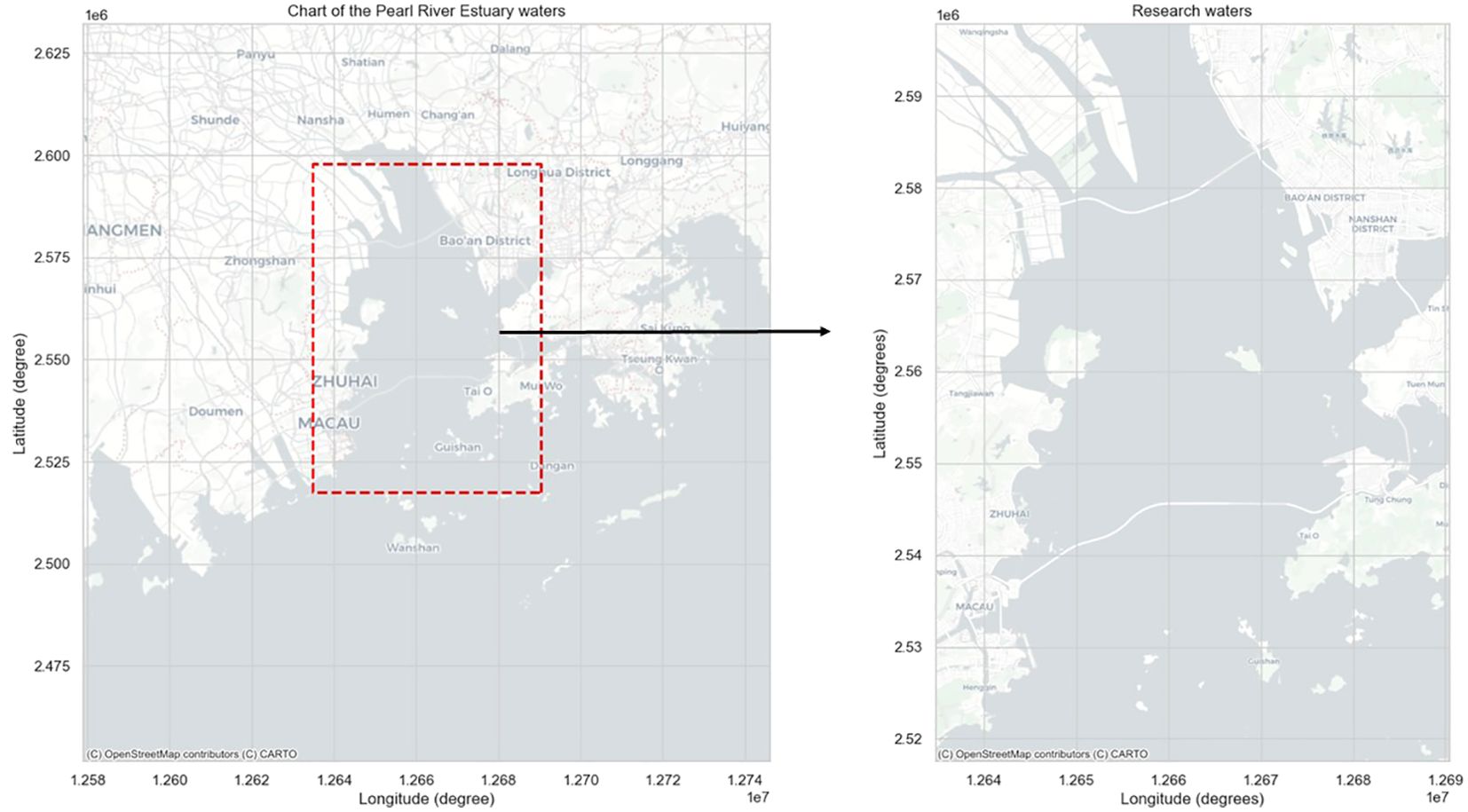
Figure 1. Location of the research area in Pearl River Estuary.

2.2 AIS data

According to the guidelines by IMO, AIS data should include three categories of information: (1) static data, including the unique vessel identifiers (MMSI), vessel name, call sign, length, width, and vessel type; (2) dynamic data, referring to trajectory and status information generated during the vessel’s navigation, including latitude, longitude, speed, and course; (3) navigational data, describing the navigational state of vessel, including draft, status, and destination.

The time intervals for different types of data vary. For static and navigational data, the message is reported generally every 6 minutes or updated immediately when queried. However, the update of dynamic data is usually less than 3 minutes, with specific intervals determined by the vessel’s current heading and speed. Currently, AIS equipment have been installed on most vessels in navigable waters, providing their real-time status.

The collected dataset in this research covers the time span from August 16, 2023, to November 16, 2023 in the research area. The dataset contains a total of 15,921,338 records, featuring various types of vessels. However, due to the limited amount of data for other vessel types, such as tugs, high speed crafts, law enforcement vessels, etc., this research focuses on the behavior of the main four types of vessels in the area, being cargo ships (2,263,519 records), fishing vessels (1,957,002 records), tankers (2,795,298 records), and passenger ships (8,902,264 records). The trajectories of these four types of vessels are shown in Figure 2.

Figure 2

Figure 2. Trajectories overview of four types of vessels in the research area. (Different colors indicate the trajectories of different vessels according to their MMSI number.) (A) Cargo ships, (B) Tankers, (C) Fishing vessels, (D) Passenger ships.

Generally comparing the trajectories, it can be observed that the density of cargo ship trajectories is high and concentrated, indicating that these vessels primarily transport goods on fixed routes between ports. Similarly with fixed routes, the trajectories of passenger ships are concentrated and regular with little variation between voyages. The trajectories of tankers are wider and have a larger distribution range, suggesting that tankers have high requirements for the width of shipping lanes and tend to avoid areas with dense ship traffic to ensure safety. However, only for the trajectories of fishing vessels, they are randomly distributed, indicating that their activities are greatly influenced by the distribution of fishery resources. Thus, the behavior of fishing vessels presents strong flexibility.

2.3 Data preprocessing

To proceed with the vessel behavior analysis and vessel classification, the collected AIS data is preprocessed by the following three steps.

(1) Missing value removal. Some trajectory data lack critical static information, such as vessel length, width, MMSI, and vessel type. Since this data cannot be repaired, records with missing values were removed.

(2) Outlier removal. After removing the messages with missing values, it is necessary to address outliers in the collected data. In this experiment, the main outliers to be fixed include the ship’s speed and position. The defined outliers include sudden increases or decreases in data values, trajectory points that deviate from the expected path, and gaps in the trajectory. The outliers at the beginning or end of a trajectory segment are removed directly, which does not affect the quality for analysis. If outliers are found within a segment, linear interpolation is used to replace them with the average of the two surrounding points. If multiple consecutive outliers are present, they are treated as missing values and corrected using linear interpolation based on the fitted trajectory curve, considering the spacing between trajectory points. This paper uses the speed value and the time interval between two adjacent data points to determine whether there are missing values. First, the value of speed indicates the status of the ship. For instance, when the speed is mostly around 0.1 kn during a trajectory segment, the ship is not indeed sailing on its own, in which the speed is probably caused by wind and current. Thus, these data are removed. In this paper, the threshold of speed during data removal is set as 1 kn. Additionally, if the time interval between two adjacent data points is greater than 3 minutes and less than 10 minutes, missing values are considered to exist between them. The information of ship’s position and speed will be checked. If more than five points of incorrect position or speed appear consecutively within the same trajectory segment, this segment will be removed.

(3) Trajectory segmentation. After processing the AIS data, trajectories are segmented according to the vessel’s navigational status. Since this information in the collected data is mostly missing, the vessel’s navigational status is defined according to the speed. Once the speed exceeds 1 knot, it is deemed as an underway vessel. Only the segments including underway vessels are retained, and trajectory segments with fewer than 100 data points are removed.

After preprocessing the AIS data, this paper keeps 8,200 sets of ship data, including 2,000 sets for cargo ships, tankers, and passenger ships, and 2,200 sets for fishing vessels.

3 Research approach

This paper combines the concepts of ensemble learning with BP neural networks and the AdaBoost algorithm, using AdaBoost to combine n BP neural networks into a strong classifier. By improving the BP neural network, the classification of cargo ships, fishing vessels, tankers, and passenger ships is achieved. The overview of the proposed methodology is shown in Figure 3.

Figure 3

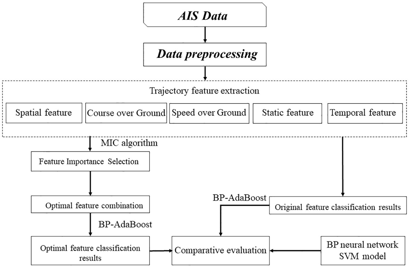
Figure 3. Overview of the proposed methodology.

3.1 Behavior feature extraction

To accurately reveal the differences in behavior trajectories among various types of vessels, five main features are extracted from the AIS data: spatial feature, COG (Course of Ground), SOG (Speed over Ground), static feature, and temporal feature. These features can be used to identify vessel types.

3.1.1 Spatial feature

In this paper, the spatial feature of ship trajectory is described from two aspects, being the sailing distance and the longitude and latitude span. Due to the operational characteristics of vessels, cargo ships and tankers do not require multiple round trips to ports within a certain period of time, such as one day. Thus, their voyages usually cover a large span of latitude and longitude with a relatively short sailing distance, compared to fishing vessels and passenger ships. In contrast, fishing vessels and passenger ships frequently travel between several certain docks or fishing grounds in one single day due to their operational demands, leading to a small span of latitude and longitude, but with a longer sailing distance.

Based on the Haversine formula for spherical distance calculation, the sailing distance can be computed as follows:

$$\mathit{d}=\mathbf{2}\mathit{r} *\mathit{s}\mathit{i}{\mathit{n}}^{-\mathbf{1}}\sqrt{{\left(\mathit{sin}\frac{\mathit{\Delta }{\mathit{\phi }}^{\prime }}{\mathbf{2}}\right)}^{\mathbf{2}}+\mathit{c}\mathit{o}\mathit{s}{{\mathit{\phi }}^{\prime }}_{\mathbf{1}}*\mathit{c}\mathit{o}\mathit{s}{{\mathit{\phi }}^{\prime }}_{\mathbf{2}}{(\mathit{sin}\frac{\mathit{\Delta }{\mathit{\gamma }}^{\prime }}{\mathbf{2}})}^{\mathbf{2}}}$$

where d represents the distance between two trajectory points; r is the radius of the Earth, take 6371.393 km; Δφ′=| ${{\phi }^{\prime }}_1$− ${{\phi }^{\prime }}_2$|, Δ $\gamma$′=| $\gamma {\text{'}}_1$− $\gamma {\text{'}}_2$|, (${{\phi }^{\prime }}_1$, $\gamma {\text{'}}_1$) and (${{\phi }^{\prime }}_2$, $\gamma {\text{'}}_2$)refers to the positions of the two trajectory points, expressed in radians.

The longitude span and the latitude span are:

$$|\mathit{L}\mathit{O}\mathit{N}\_\mathit{S}\mathit{P}\mathit{A}\mathit{N}|=|\mathit{L}\mathit{O}{\mathit{N}}_{\mathit{M}\mathit{A}\mathit{X}}-\mathit{L}\mathit{O}{\mathit{N}}_{\mathit{M}\mathit{I}\mathit{N}}|$$

$$|\mathit{L}\mathit{A}\mathit{T}\_\mathit{S}\mathit{P}\mathit{A}\mathit{N}|=|\mathit{L}\mathit{A}{\mathit{T}}_{\mathit{M}\mathit{A}\mathit{X}}-\mathit{L}\mathit{A}{\mathit{T}}_{\mathit{M}\mathit{I}\mathit{N}}|$$

where $LO{N}_{MAX}$ and $LA{T}_{MAX}$ are the maximum values of longitude and latitude in a trajectory segment, $LO{N}_{MIN}$ and $LA{T}_{MIN}$ are the minimum values of longitude and latitude in the same trajectory segment.

3.1.2 Course over ground

To extract COG features, this study design a method to determine whether a vessel is turning, as described in Algorithm 1. First, the COG change between each data point is calculated. Points with COG changes exceeding a certain threshold are marked as potential turning points. Next, n consecutive potential turning points are marked as a potential turning segment. Finally, the COG changes within the potential turning segment are checked against the threshold criteria, and those that meet the criteria have all their potential turning points marked as actual turning points.

Algorithm 1. COG feature extraction algorithm.

The extraction is primarily divided into the following four steps:

Step 1: Initialize thresholds: 1) threshold COG change: This threshold determines whether the COG change is significant enough to mark a point as a potential turning point. It is set to a COG change of at least 0.8 between two consecutive data points. 2) threshold consecutive points: This threshold establishes the required number of consecutive potential turning points to mark a potential turning segment, set to at least 10 consecutive turning points. 3) threshold segment change: This threshold confirms the turning segment by evaluating the total COG change within that segment, set to a minimum change of 5 degrees.

Step 2: Mark potential turning points: Iterate through each heading data point and calculate the COG change between the current point and the previous one. If the change exceeds threshold COG change, mark the point as a potential turning point.

Step 3: Mark potential turning segments: Identify n consecutive potential turning points, ensuring they are continuous (i.e., the index difference between adjacent points is 1). These points are then labeled as a potential turning segment.

Step 4: Confirm turning segments: For each potential turning segment, calculate the total COG change within the segment. If this change exceeds threshold segment change, confirm it as an actual turning segment and mark all points within it as turning points.

The method extracts the maximum turning angle, average turning speed, and the average change of COG over the entire trajectory segment. These variables comprehensively describe the feature of ship behavior in the aspect of course control.

3.1.3 Speed over ground

Different types of vessels exhibit varying speed distributions. By analyzing these speed differences, one can preliminarily assess vessel behavior, providing classification features for vessel target classification. To describe the speed over ground, the minimum, maximum, upper quartile, median, lower quartile, mean and standard deviation of the speeds are extracted.

3.1.4 Static feature

Static features primarily reflect the size of the vessels. Generally, fishing vessels and passenger ships are smaller, while cargo ships and tankers are larger. In this study, the aspect ratio of the vessel is used to represent its size:

$$\mathit{A}\mathit{s}\mathit{p}\mathit{e}\mathit{c}\mathit{t} \mathit{R}\mathit{a}\mathit{t}\mathit{i}\mathit{o} = \mathit{L}/\mathit{W}$$

where L is the length of the ship and W is the width of the ship.

3.1.5 Temporal feature

Temporal features primarily consist of time-related attributes, including acceleration and COG change rate. Generally, cargo ships and tankers exhibit slow speed changes and low COG change frequencies, while fishing vessels and passenger ships, due to their operational characteristics, frequently change direction and experience rapid speed variations.

The acceleration and the rate of COG change are calculated by

$$\mathit{a}=\frac{{\mathit{\Delta }}_{\mathit{v}}}{{\mathit{\Delta }}_{\mathit{t}}}$$

$$\mathit{C}=\frac{\mathit{C}\mathit{O}{\mathit{G}}_{\mathit{d}\mathit{i}\mathit{f}\mathit{f}}}{{\mathit{\Delta }}_{\mathit{t}}}$$

where $a$ is the acceleration; ${\Delta }_v$ is the velocity difference between the upper and lower data points; ${\Delta }_t$ is the data collection interval; C is the rate of COG change; $CO{G}_{diff}$ is the difference between the upper and lower data points for the Course of ground.

3.2 Feature importance selection

Maximal Information Coefficient (MIC), is proposed by Reshef et al. (2011) to measure the degree of association between two variables, X and Y, regardless of whether the relationship is linear or nonlinear. It is commonly used in machine learning for feature selection. Its value ranges from 0 to 1, with higher values indicating stronger correlations between variables. MIC quantifies the strength of dependence between variables, offering a consistent metric across various types of associations. Compared to commonly used feature selection methods like Pearson correlation and threshold correlation, MIC handles nonlinear data more effectively, offers lower computational complexity, and provides better robustness.

Therefore, MIC possesses two main advantages for this research. Firstly, the MIC metric is versatile, which can identify both linear and nonlinear functional relationships (including exponential and periodic), as well as non-functional relationships. Secondly, the MIC metric is balanced. For functionally or non-functionally related variables with the same noise level, MIC yields similar values. Thus, MIC can be used to compare the strength of the same relationship over time as well as different relationships across contexts.

3.3 Vessel classification based on behavior features

To address issues like slow convergence rate and susceptibility to local optima inherent in BP neural networks, the AdaBoost algorithm is used to improve the BP neural network, combining weak classifiers into a strong classifier through the concept of ensemble learning. The two main optimization challenges are primarily addressed. Firstly, it integrates BP neural networks with the AdaBoost algorithm, capitalizing on the BP networks’ capability for multi-output nodes to enable AdaBoost to tackle multi-class classification tasks. Secondly, instead of merely measuring classification errors when assessing the learning outcomes against the desired classification results, the paper calculates the classification error rate. This rate is then utilized to refine the weights of the training samples and the influence of weak classifiers, which in turn enhances the accuracy of the classification process.

When solving a multi-classification problem using the BP-AdaBoost algorithm, assume that the given multi-class dataset is $\text{T}=\{(x_1,y_1),(x_2,y_2),\dots ,(x_n,y_n)\},x_i\in R^n$, and the sample data is $y_i\in [1,2,\dots ,n]$, and the specific improvement of the BP- AdaBoost algorithm is as follows:

1. Calculate the weights of the training data input to the first weak classifier $D_i$:

$${\mathit{D}}_{\mathit{i}}=({\mathit{w}}_{\mathbf{1},\mathbf{1}},\dots ,{\mathit{w}}_{\mathbf{1},\mathit{i}},\dots ,{\mathit{w}}_{\mathbf{1},\mathit{n}})=\frac{\mathbf{1}}{\mathit{n}},\mathit{i}=\mathbf{1},\mathbf{2},\dots ,\mathit{n}$$

2. Train the BP neural network using the training dataset to obtain weak classifiers. The output of these weak classifiers can be expressed by the following equation:

$${\mathit{G}}_{\mathit{n}}(\mathit{x}):\mathit{x}\to \{\mathbf{1},\mathbf{2},\dots ,\mathit{K}\}$$

where N represents the number of categorized species, n = $1,2,\dots ,\text{N}$(3) Calculate the classification error rate $e_n$ of the weak classifier output $G_n(x)$:

$${\mathit{e}}_{\mathit{n}}=\frac{\mathbf{1}}{\mathit{n}}{\displaystyle \sum _{\mathit{i}=\mathbf{1}}^{\mathit{n}}\mathit{I}}({\mathit{G}}_{\mathit{n}}({\mathit{x}}_{\mathit{i}})\ne {\mathit{y}}_{\mathit{i}})$$

where $y_i$ is the expected classification result.

4. Calculate the weights of the generated weak classifiers in the final strong classifier $a_n$:

$${\mathit{\alpha }}_{\mathit{n}}=\frac{\mathbf{1}}{\mathbf{2}}\mathit{ln}\frac{\mathbf{1}-{\mathit{e}}_{\mathit{n}}}{{\mathit{e}}_{\mathit{n}}}+\mathit{l}\mathit{n} (\mathit{K}-\mathbf{1})$$

5. Update the sample data weights $D_{n+1}$ and calculate the output of the next weak classifier.

$$\begin{array}{c}{\mathit{D}}_{\mathit{n}+\mathbf{1}}=({\mathit{w}}_{\mathit{n}+\mathbf{1},\mathbf{1}},\cdots ,{\mathit{w}}_{\mathit{n}+\mathbf{1},\mathit{i}},\cdots ,{\mathit{w}}_{\mathit{n}+\mathbf{1},\mathit{m}})\\ {\mathit{w}}_{\mathit{n}+\mathbf{1},\mathit{i}}=\frac{{\mathit{w}}_{\mathit{n},\mathit{i}}}{{\mathit{Z}}_{\mathit{n}}}\mathit{e}\mathit{x}\mathit{p}[-{\mathit{\alpha }}_{\mathit{n}}{\mathit{f}}_{\mathit{i}}{\mathit{G}}_{\mathit{n}}({\mathit{x}}_{\mathit{i}})]\end{array}$$

When the prediction is correct, $f_i$= 1; when the prediction is wrong, $f_i$= -1.

where $Z_n$ is the normalization coefficient, which ensures that the sum of the distribution weights equals 1 while keeping the weight ratios unchanged. Its mathematical expression is as follows:

$${\mathit{z}}_{\mathit{n}}={\displaystyle \sum _{\mathit{i}=\mathbf{1}}^{\mathit{n}}{\mathit{w}}_{\mathit{n},\mathit{i}}}\mathit{e}\mathit{x}\mathit{p}(-{\mathit{a}}_{\mathit{n}}\mathit{f}{\mathit{G}}_{\mathit{i}}({\mathit{x}}_{\mathit{i}}))$$

6. Normalize the data results, and the outputs of the N weak classifiers are combined to obtain a strong classifier $h(x)$

$$\mathit{h}(\mathit{x})=\mathit{s}\mathit{i}\mathit{g}\mathit{n}({\displaystyle \sum _{\mathit{n}=\mathbf{1}}^{\mathit{M}}{\mathit{a}}_{\mathit{n}}}*\mathit{f}({\mathit{a}}_{\mathit{n}},{\mathit{G}}_{\mathit{n}}(\mathit{x})))$$

where $Sign$ denotes the sign function, which is used to convert the result of the weighted sum into the final classification decision; M is the total number of base classifiers; $a_n$ is the weight of the nth base classifier, which denotes the importance of that classifier; and $G_n(x)$ is the nth base classifier that produces a classification result for input $\text{x}$.

To evaluate the proposed classifier, Accuracy, Precision, Recall and $F_1-score$ are used as classification metrics in this research.

$$\mathit{A}\mathit{c}\mathit{c}\mathit{u}\mathit{r}\mathit{a}\mathit{c}\mathit{y}=\frac{\mathit{T}\mathit{P}+\mathit{T}\mathit{N}}{\mathit{T}\mathit{P}+\mathit{T}\mathit{N}+\mathit{F}\mathit{P}+\mathit{F}\mathit{N}}$$

$$\mathit{P}\mathit{r}\mathit{e}\mathit{c}\mathit{i}\mathit{s}\mathit{i}\mathit{o}\mathit{n}=\frac{\mathit{T}\mathit{P}}{\mathit{T}\mathit{P}+\mathit{F}\mathit{P}}$$

$$\mathit{R}\mathit{e}\mathit{c}\mathit{a}\mathit{l}\mathit{l}=\frac{\mathit{T}\mathit{P}}{\mathit{T}\mathit{P}+\mathit{F}\mathit{N}}$$

$${\mathit{F}}_{\mathbf{1}}-\mathit{s}\mathit{c}\mathit{o}\mathit{r}\mathit{e}=\frac{\mathbf{2}\times \mathit{P}\mathit{r}\mathit{e}\mathit{c}\mathit{i}\mathit{s}\mathit{i}\mathit{o}\mathit{n}\times \mathit{R}\mathit{e}\mathit{c}\mathit{a}\mathit{l}\mathit{l}}{\mathit{P}\mathit{r}\mathit{e}\mathit{c}\mathit{i}\mathit{s}\mathit{i}\mathit{o}\mathit{n}+\mathit{R}\mathit{e}\mathit{c}\mathit{a}\mathit{l}\mathit{l}}$$

where, $TP,FP,TN,FN$ denote True positive, False positive, False negative, and True negative, respectively.

4 Experimental analysis

The proposed vessel classification method is tested using the collected dataset in the research area as described in Section 2. 70% of the data serves as the training set, while the rest is for testing. In the experiments of this paper, the BP neural network has 4 nodes in the output layer and 15 nodes in the hidden layer. The number of nodes in the input layer is determined by the number of input features. The maximum number of iterations is set to 500, the error threshold is set to 1e-3, and the learning rate is 0.01. The network weights and biases for the input and output layers are optimized using the ant colony optimization algorithm. The classification results are presented in this section, followed by a comparative analysis with the SVM and BP single classifier models.

4.1 Behavior feature extraction and selection

Analyzing the vessel behavior in the research area by the proposed method in Section 3.1, the behavior features are extracted. The feature distribution for various types of ships, and their numbering in feature selection are shown Figures 4–8.

Figure 4

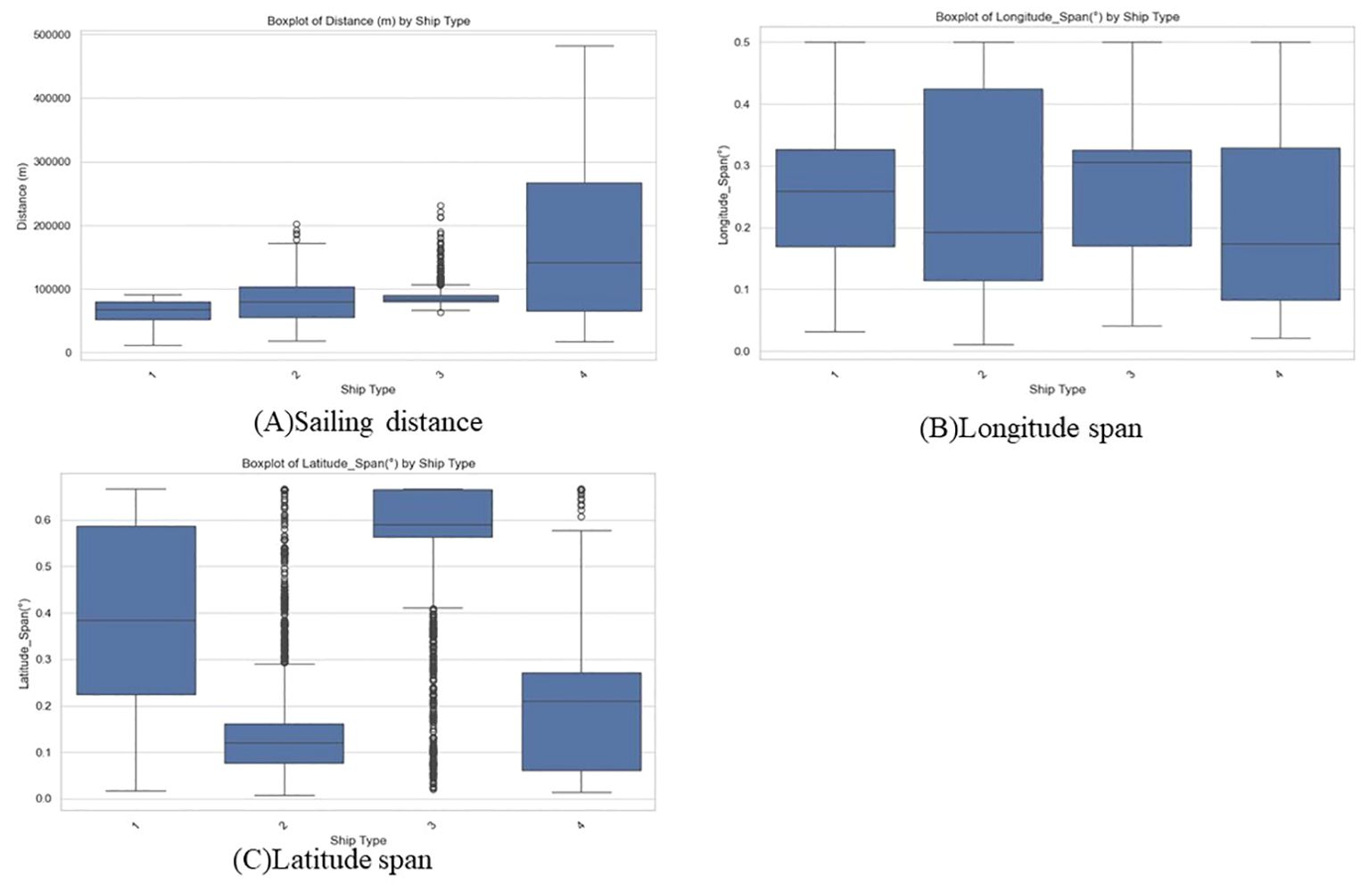
Figure 4. Distribution of spatial feature. (Box 1 represents cargo ship, box 2 represents fishing vessel, box 3 represents tanker, and box 4 represents passenger ship.). (A) Sailing distance, (B) Longitude span, (C) Latitude span.

Figure 5

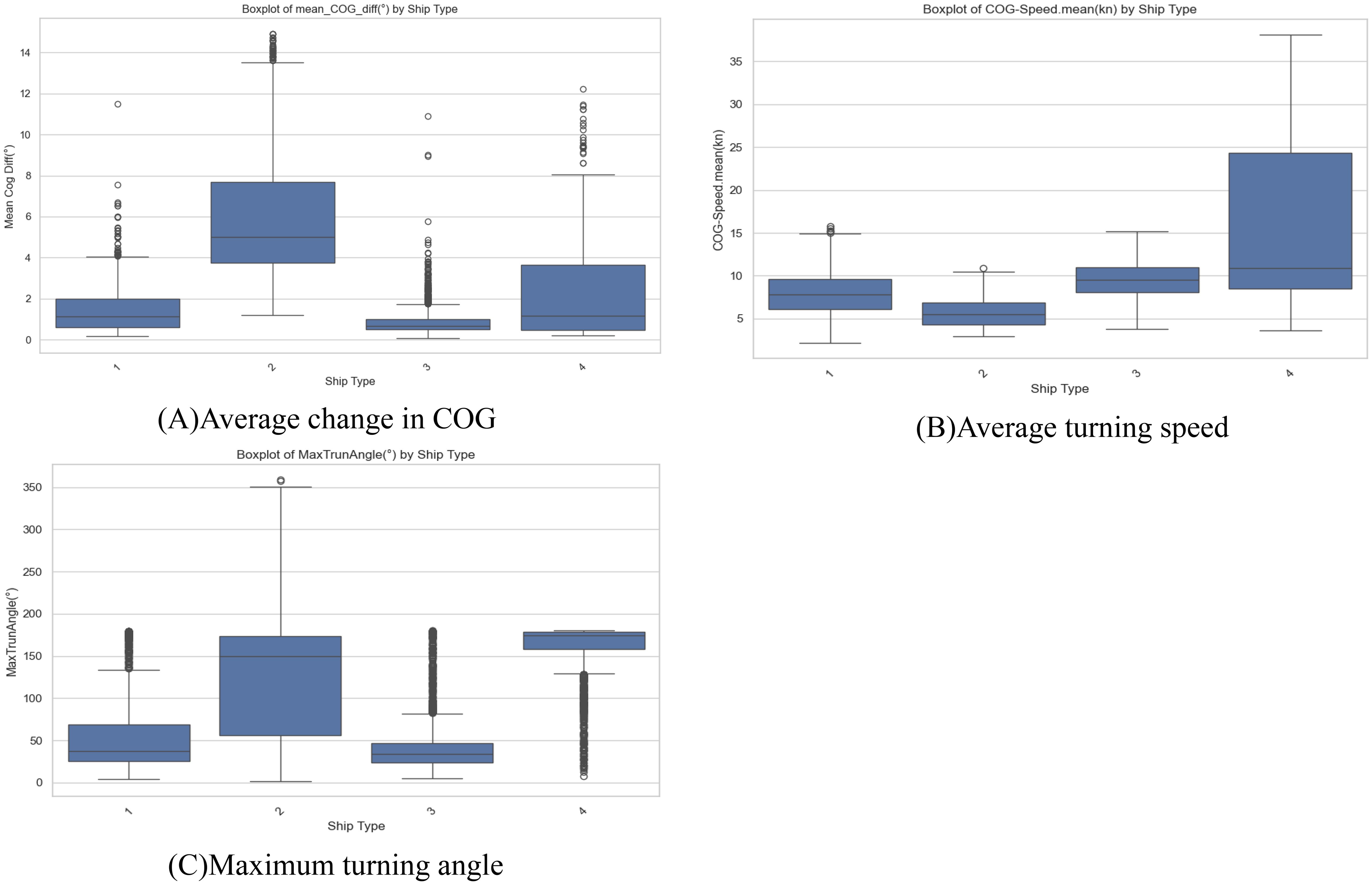
Figure 5. Distribution of COG. (Box 1 represents cargo ship, box 2 represents fishing vessel, box 3 represents tanker, and box 4 represents passenger ship.). (A) Average change in COG, (B) Average turning speed, (C) Maximum turning angle.

Figure 6

Figure 6. The Speed over Ground distributions of four types of vessels. (A) Cargo Ship, (B) Fishing vessel, (C) Tanker, (D) Passenger Ship.

Figure 7

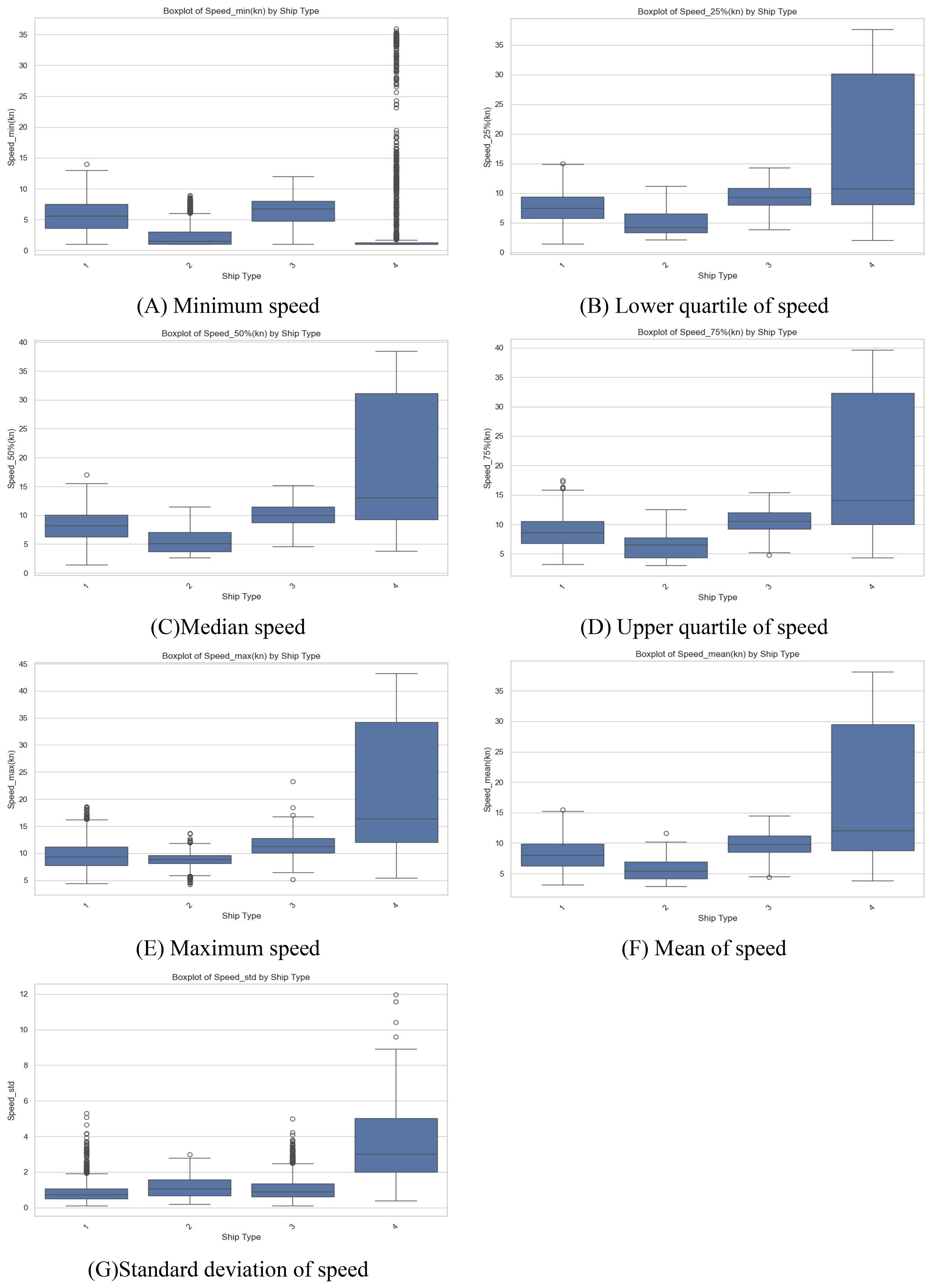
Figure 7. Distribution of SOG. (Box 1 represents cargo ship, box 2 represents fishing vessel, box 3 represents tanker, and box 4 represents passenger ship.). (A) Minimum speed, (B) Lower quartile of speed, (C) Median speed, (D) Upper quartile of speed, (E) Maximum speed, (F) Mean of speed, (G) Standard deviation of speed.

Figure 8

Figure 8. Distribution of static and temporal features. (Box 1 represents cargo ship, box 2 represents fishing vessel, box 3 represents tanker, and box 4 represents passenger ship.). (A) Ship Aspect Ratio, (B) Average acceleration of ship, (C) Maximum acceleration of ship, (D) Average COG_change rate of ship, (E) Maximum COG_change rate of ship.

4.1.1 Spatial feature

In the Spatial feature shown in Figure 4, fishing vessels and passenger ships have the longest sailing distance. This is due to their operational feature, as passenger ships frequently travel back and forth between ports each day, resulting in a sailing distance significantly greater than that of other vessels. The distribution of tankers and cargo ships is similar, but tankers show a tighter distribution. In longitude span, fishing vessels have the largest span, while tankers have the largest latitude span.

4.1.2 Course over ground

In the COG feature in Figure 5, fishing vessels exhibit the highest frequency of heading changes, which is again due to their operational characteristics, as they need to maneuver repeatedly within the same fishing grounds to catch fish. In terms of turning angles, fishing vessels have the largest turning angles, while passenger ships maintain their maximum turning angles over a larger range. Additionally, since passenger ships are faster than other types of vessels, they rank first in average turning speed.

4.1.3 Speed over ground

Kernel density estimation (KDE) is a non-parametric statistical method that estimates the probability distribution by placing a kernel function around each data point and summing these kernels. The KDE plot addresses a fundamental data smoothing issue, allowing for inference about the population based on a limited sample. The KDE distribution plot enables visualization and assessment of the distribution of feature variables in both the training and testing datasets. The KDE distributions of Speed over Ground among four types of vessels are presented in Figure 6.

The kernel density plot of speed reveals that the speed of most fishing vessels is below 7.5kn, as their speeds will remain low because they are carrying out fishing operations; the speed distributions of cargo ships and tankers are similar, but the average speeds of tankers are greater than that of cargo ships, and the speeds of tankers are more stable; the speeds of passenger ships are mainly distributed in two intervals, below and above 20kn, where the speeds of ships over Ships above 20kn generally have smaller sizes and low drafts, and passenger ships below 20kn have larger sizes and deeper drafts. The detailed Speed over Ground is shown in Figure 7.

It can be observed that the speed over ground reveals that passenger ships significantly outpace other types of vessels. Among the four types of ships, fishing vessels have the slowest speeds, while the speed distributions of cargo ships and tankers are similar, with the tanker being slightly faster than the cargo ship.

4.1.4 Static and temporal features

From Figure 8, it can be seen that in the distribution of static features, the distributions of cargo ships and tankers are similar, with tankers having a larger aspect ratio than cargo ships, while passenger ships and fishing vessels have smaller aspect ratio. In the distribution of temporal features, passenger ships have the largest maximum and average accelerations. In terms of average COG change rate and maximum COG change rate, fishing vessels rank first.

Analyzing the behavior features from an integrated perspective, passenger ships and fishing vessels exhibit similar behaviors, while cargo ships and tankers are relatively comparable. Fishing vessels are characterized by slower speeds, higher turning frequencies, and longer sailing distances. In contrast, passenger ships have the fastest speeds and the greatest sailing distances. Cargo ships and tankers are larger in size, with the main differences being speed and COG; tankers are generally faster than cargo ships, have more stable COG, and their sailing distances are also slightly greater.

Applying the MIC algorithm to assess the feature importance, the results are shown in Figure 9. The features are ordered as follows: sailing distance, longitude span, latitude span, average change in COG, average turning speed, maximum turning angle, minimum speed, upper quartile of speed, median speed, lower quartile of speed, maximum speed, mean of speed, standard deviation of speed, ship aspect ratio, average acceleration of ship, maximum acceleration of ship, Average COG_change rate of ship and Maximum COG_change rate of ship.

Figure 9

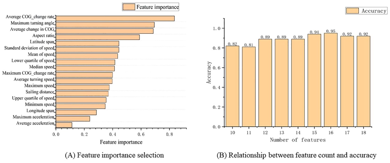
Figure 9. The selection results of feature importance and the relationship between the number of features and accuracy. (A) Feature importance selection, (B) Relationship between feature count and accuracy.

Figure 9A shows that the feature with the highest MIC value is Average COG_change rate of ship. For fishing vessels, their COG changes rapidly, resulting in a higher average rate than other ship types. The second and third rankings are the average change in COG and the maximum turning angle, indicating that COG-related features contribute more to classification than those related to other information.

Using the MIC algorithm, 16 features are retained: sailing distance, longitude span, latitude span, average change in COG, average turning speed, maximum turning angle, minimum speed, upper quartile of speed, median speed, lower quartile of speed, maximum speed, mean of speed, standard deviation of speed, ship aspect ratio, average COG_change rate of ship, Maximum COG_change rate of ship, while the remaining two features are removed, i.e., average acceleration of ship and maximum acceleration of ship, simplifying the computational complexity.

From Figure 9B, we can observe that the model’s accuracy is highest when the number of features is 16. It is important to note that the model’s classification accuracy refers to the ratio of correctly classified samples to the total number of samples in the test set, providing a direct evaluation of the model’s classification performance. Although the analysis suggests that the top 16 features form the best combination, considering the impact of different feature combinations on the model’s classification accuracy and the differences in training efficiency, this study will optimize the best feature combination and its corresponding classification model from five schemes: top 10 features, top 12 features, top 14 features, top 16 features, and all 18 features.

4.2 Classification results and analysis

Using the 18 original features and the selected features, this paper constructs the BP-AdaBoost model to classify the four types of vessels and analyzes the classification results. To obtain the optimal model under different feature combinations, the number of weak classifiers needs to be determined first. Taking 16 features as an example, Figure 10 displays the bar chart showing the relationship between the number of weak classifiers and accuracy under various conditions.

Figure 10

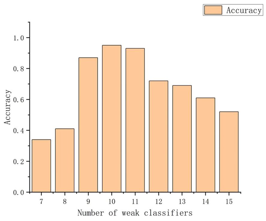
Figure 10. The relationship between the number of weak classifiers and accuracy.

Figure 10 shows that the classification accuracy is highest when the number of weak classifiers is set to 10; thus, this study uses 10 as the number of weak classifiers.

The experimental results for the five combination schemes are presented in Table 1. From Table 1, it can be seen that the classification accuracy for the top 16 feature variables reaches near its maximum, with cross-entropy and gradients also close to their minimum values. However, as the number of features increases, the accuracy shows only slight improvements or remains unchanged. Since all feature variables in the combination are used for model training, increasing the number of features inevitably raises model complexity and training time. This indicates that redundant feature variables do not contribute to classification accuracy and instead prolong training time, reducing the efficiency of vessel classification. Overall, the BP-AdaBoost method based on feature selection achieves classification accuracy comparable to that of the original features, while demonstrating better classification efficiency for cargo ships, passenger ships, fishing vessels, and tankers.

Table 1

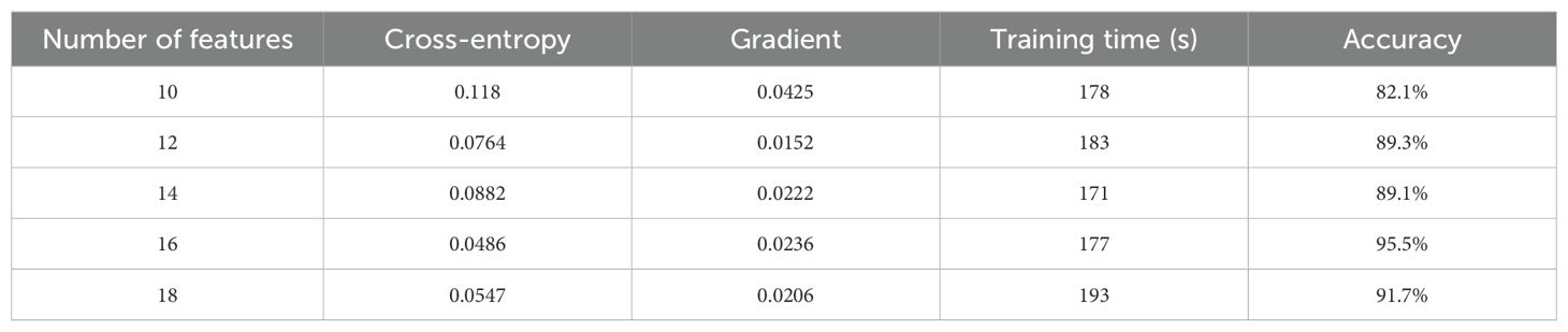
Table 1. Comparison of classification accuracy and efficiency for different feature combinations.

After training, the optimal BP-AdaBoost model and the best feature combination are obtained. The prediction results for the test set appear in a confusion matrix, an effective visual tool for evaluating the performance of classification algorithms in supervised learning. As shown in Figure 11, the overall predictions for each category align along the diagonal of the confusion matrix, which indicates that the BP-AdaBoost model accurately identifies the vessel types.

Figure 11

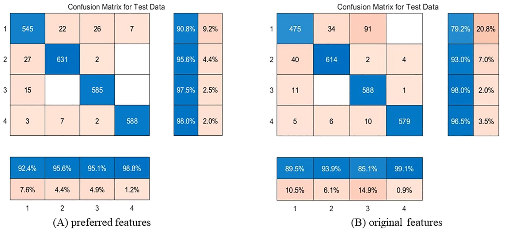
Figure 11. Confusion Matrix of preferred features and original features. (Category 1 is for cargo ship, category 2 is for fishing vessel, category 3 is for tanker, and category 4 is for passenger ship.). (A) preferred features, (B) original features.

In the selected area, cargo ships and fishing vessels, as well as tankers and cargo ships, are easily confused. This is mainly because tankers and cargo ships generally follow the same routes, with similar SOG and COG, leading to some tankers being misidentified as cargo ships. Fishing vessel operates mainly in two states: the fishing state, where they have slower speeds and higher turning rates, and the non-fishing state, where their speeds increase and COG changes decrease. This behavior can resemble that of a cargo ship, resulting in some fishing vessels being misclassified as a cargo ship.

To further compare the classification performance of the preferred features and the original features, Precision, Recall, $F_1-score$, and AUC curve are used as evaluation metrics. The evaluation results are listed in Table 2.

Table 2

Table 2. Classification and recognition effect of each type of ship target.

Overall, the preferred feature group performs better, accurately identifying different types of vessels with an overall classification accuracy of 95.5%. The precision metrics for passenger ships, cargo ships, fishing vessels, and tankers all exceed 90%, and both the $F_1-score$ and recall also exceed 90%. The AUC values for all four vessel types exceed 0.98, indicating that the classifier performs well. Compared to the original feature set, the overall accuracy increases by 3.8%. This demonstrates that removing redundant features enhances the model’s classification accuracy both overall and locally.

Locally, after removing the redundant features of maximum acceleration and mean acceleration, the classification accuracy for the four types of vessels improved to varying degrees. After feature selection, the classification accuracy for cargo ships increased by 11.6%, and the recall for tankers improved by 10%. This indicates a reduction in cargo ships being misclassified as tankers, suggesting that the classification accuracy of vessels improved after feature selection.

4.3 Comparative analysis

To further evaluate the method proposed in this chapter, multiple comparative experiments are conducted, including SVM and BP single classifier models commonly used for classification tasks in machine learning. To ensure consistent feature counts, both SVM and BP neural networks exclude features average acceleration of ship and maximum acceleration of ship, while the model testing results are presented in Table 3.

Table 3

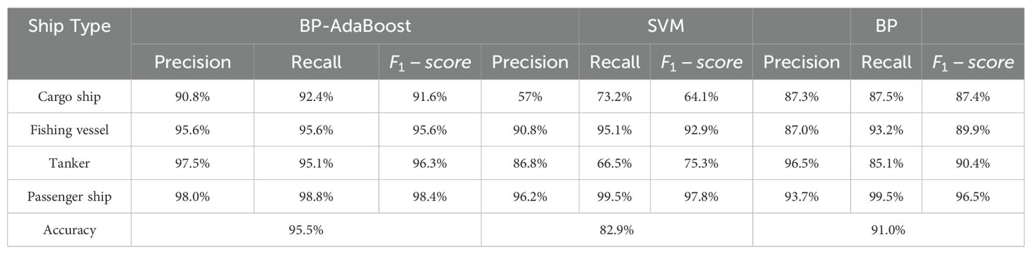
Table 3. Indicators of Comparative Experiments.

From the perspective of overall accuracy, the BP-AdaBoost model based on the best feature combination outperforms the other two models in classification accuracy, with an improvement of 12.6% over SVM and 4.5% over the BP neural network. Next, precision, recall, and F1-score are used to quantitatively evaluate the test results. The comparison shows that the BP-AdaBoost model effectively performs ship target classification across the four ship types, achieving an overall accuracy of 95.5%. Additionally, the BP neural network performs excellently in identifying tankers and passenger ships, with classification accuracies exceeding 93%. However, the classification performance for cargo ships and fishing vessels is weaker, with precision around 87%. This is due to the similarities in movement patterns between cargo ships and other types, leading to some confusion in classification. By analyzing recall, it is found that the recall for fishing vessels and passenger ships is higher than that for cargo ships and tankers, indicating that more samples are misclassified as cargo ships and tankers. In contrast, the SVM model performs well in classifying fishing vessels, tankers, and passenger ships, with classification precision exceeding 86%, but struggles with classifying cargo ships, with precision only around 57%. The recall for cargo ships and tankers are only 73.2% and 66.5%, respectively, suggesting that cargo ships are easily confused with tankers. The experimental results show that traditional machine learning algorithms perform poorly in multi-type ship classification.

From the experimental results, the proposed BP-AdaBoost classification model effectively achieves rapid ship classification on a small dataset, accurately distinguishing between passenger ships, cargo ships, fishing vessels, and tankers. To improve the confusion between certain ship types, incorporating additional COG features, temporal features, and a more diverse sample library would help further enhance the model’s performance. Applying the proposed method using AIS data, the vessels engaged in fishing activities can be recognized based on their behavior features. Comparing the recognition results to their marked vessel types, the vessels potentially involved in illegal fishing activities can be identified. This way, the fishing activities can be better monitored and the marine resources are expected to be better protected.

5 Discussion

To classify ship types using historical AIS data, a BP-AdaBoost classification algorithm is proposed, effectively categorizing cargo ships, fishing vessels, tankers, and passenger ships. The process start with AIS data preprocessing, where entries with critical missing data are removed and anomalies are corrected. Static, behavioral, and temporal features of the ships are analyzed and extracted. The MIC algorithm is then employed for feature selection, identifying five feature combinations for classification experiments. The BP-AdaBoost algorithm achieve an optimal feature combination of 16 dimensions, with an overall classification accuracy of 95.49% for the four ship types: cargo ships at 90.8%, fishing vessels at 95.6%, tankers at 97.5%, and passenger ships at 98%. Compared to standalone BP neural network and SVM classification models, BP-AdaBoost outperform them in precision, recall, and other metrics. The classification accuracy is 4.5% higher than that of the BP neural network and 12.6% higher than the SVM model. The results show that this method can effectively detect abnormal vessels that may forge or improperly transmit AIS messages to evade monitoring. This has significant implications for maritime supervision, environmental stability, and combating illegal fishing, proving the effectiveness of the proposed method.

In the future, the behavior of more vessel types can be investigated with VMS data, remote sensing imagery, or radar images to enhance ship target recognition accuracy. Thus, the vessels engaged in fishing activities can be more accurately recognized to identify illegal fishing activities and protect the fishery resources.

Data availability statement

The original contributions presented in the study are included in the article/supplementary material, further inquiries can be directed to the corresponding author/s.

Author contributions

XH: Conceptualization, Formal Analysis, Investigation, Methodology, Software, Visualization, Writing – original draft. YZ: Conceptualization, Data curation, Funding acquisition, Methodology, Supervision, Validation, Writing – review & editing. JW: Project administration, Supervision, Writing – review & editing. LC: Resources, Writing – review & editing. KL: Writing – review & editing.

Funding

The author(s) declare that financial support was received for the research, authorship, and/or publication of this article. The research is supported by the Natural Science Foundation of Hubei Province, China (Grant No. 2024AFB239).

Conflict of interest

The authors declare that the research was conducted in the absence of any commercial or financial relationships that could be construed as a potential conflict of interest.

Generative AI statement

The author(s) declare that no Generative AI was used in the creation of this manuscript.

Publisher’s note

All claims expressed in this article are solely those of the authors and do not necessarily represent those of their affiliated organizations, or those of the publisher, the editors and the reviewers. Any product that may be evaluated in this article, or claim that may be made by its manufacturer, is not guaranteed or endorsed by the publisher.

References

Cao Y., Zhao X. L., Su D. B., Cheng X., Ren H. (2023). A machine-learning-based classification method for meteorological conditions of ozone pollution. Aerosol Air Qual. Res. 23 (1), 220239. doi: 10.4209/aaqr.220239

Crossref Full Text | Google Scholar

Chi Q., Zhong-Sheng H., Yi W. (2008). “Short-term traffic flow prediction for freeway based on BP and improved BP neural network,” in 1st International Conference on Modelling and Simulation (Nanjing: Peoples R China).

Google Scholar

Damastuti N., Aisjah A. S., Masroeri A. A. (2019). “Classification of ship-based automatic identification systems using k-nearest neighbors,” in 2019 International Seminar on Application for Technology of Information and Communication (iSemantic), (Semarang, Indonesia) 331-335. doi: 10.1109/ISEMANTIC.2019.8884328

Crossref Full Text | Google Scholar

Guan Y., Zhang X., Chen S., Liu G., Jia Y., Zhang Y., et al. (2023). Fishing vessel classification in SAR images using a novel deep learning model. IEEE Trans. Geosci. Remote Sens. 61, 1–21. doi: 10.1109/tgrs.2023.3312766

Crossref Full Text | Google Scholar

Guo T., Xie L. (2022). Research on ship trajectory classification based on a deep convolutional neural network. J. Mar. Sci. Eng. 10 (5), 568. doi: 10.3390/jmse10050568

Crossref Full Text | Google Scholar

Huang H., Hong F., Liu J., Liu C., Feng Y., Guo Z. (2019). FVID: Fishing vessel type identification based on VMS trajectories. J. Ocean Univ. China 18, 403–4125. doi: 10.1007/s11802-019-3717-9

Crossref Full Text | Google Scholar

Kong Z., Cui Y., Xiong W., Yang F., Xiong Z., Xu P. (2022). Ship target identification via bayesian-transformer neural network. J. Mar. Sci. Eng. 10 (5), 577. doi: 10.3390/jmse10050577

Crossref Full Text | Google Scholar

Li H. J. (2015). “Ovarian cancer classification diagnostic model of BP networks and genetic algorithms,” in SSR International Conference on Social Sciences and Information (SSR-SSI 2015), (Tokyo, Japan).

Google Scholar

Luo D., Chen P., Yang J., Li X., Zhao Y. (2023). A new classification method for ship trajectories based on AIS data. J. Mar. Sci. Eng. 11 (9), 1646. doi: 10.3390/jmse11091646

Crossref Full Text | Google Scholar

Ma S. X., Liu S. S., Meng X. (2020). “Optimized BP neural network algorithm for predicting ship trajectory,” in 2020 IEEE 4th Information Technology, Networking, Electronic and Automation Control Conference (ITNEC), (Chongqing, China), 525-532. doi: 10.1109/ITNEC48623.2020.9085154

Crossref Full Text | Google Scholar

Pham T. D. T., Huang H. W., Chuang C. T. (2014). Finding a balance between economic performance and capacity efficiency for sustainable fisheries: Case of the Da Nang gillnet fishery, Vietnam. Mar. Policy 44, 287–294. doi: 10.1016/j.marpol.2013.09.021

Crossref Full Text | Google Scholar

Reshef D. N., Reshef Y. A., Finucane H. K., Grossman S. R., McVean G., Turnbaugh P. J., et al. (2011). Detecting novel associations in large data sets. Science 334, 1518–1524. doi: 10.1126/science.1205438

PubMed Abstract | Crossref Full Text | Google Scholar

Sheng K., Liu Z., Zhou D., He A., Feng C. (2017). Research on ship classification based on trajectory features. J. Navig. 71, 100–1165. doi: 10.1017/s0373463317000546

Crossref Full Text | Google Scholar

Sheng P., Yin J. (2018). Extracting shipping route patterns by trajectory clustering model based on automatic identification system data. Sustainability 10 (7), 2327. doi: 10.3390/su10072327

Crossref Full Text | Google Scholar

Shi X. M., Li G. N., Li K., Liu J. Y., Wang R. C., Publishing I. O. P. (2020). “Customer classification method of logistics enterprises based on BP-adaBoost,” in 3rd International Conference on Applied Mathematics, Modeling and Simulation (AMMS), (Electr Network).

Google Scholar

Wang Y., Guo J., Xu L., Li K., Li Z. (2022). “AIS Data Driven CNN-BiGRU Model for Ship Target Classification,” in Spatial Data and Intelligence (Wuhan, Peopls R China), 113–132.

Google Scholar

Xing B., Zhang L., Liu Z., Sheng H., Bi F., Xu J. (2023). The study of fishing vessel behavior identification based on AIS data: A case study of the East China sea. J. Mar. Sci. Eng. 11 (5), 1093. doi: 10.3390/jmse11051093

Crossref Full Text | Google Scholar

Yang Y., Ding K., Chen Z. (2022). Ship classification based on convolutional neural networks. Ships Offshore Struct. 17, 2715–27215. doi: 10.1080/17445302.2021.2016271

Crossref Full Text | Google Scholar

Zhang Z. G., Yin J. C., Wang N. N., Hui Z. G. (2019). Vessel traffic flow analysis and prediction by an improved PSO-BP mechanism based on AIS data. Evol. Syst. 10, 397–407. doi: 10.1007/s12530-018-9243-y

Crossref Full Text | Google Scholar

Zhong H., Song X., Yang L. (2019). “Vessel classification from space-based ais data using random forest,” in 2019 5th International Conference on Big Data and Information Analytics (BigDIA) (Kunming, China) 9-12. doi: 10.1109/BigDIA.2019.8802792

Crossref Full Text | Google Scholar

Zhou Y., Daamen W., Vellinga T., Hoogendoorn S. P. (2019). Ship classification based on ship behavior clustering from AIS data. Ocean Eng. 175, 176–187. doi: 10.1016/j.oceaneng.2019.02.005

Crossref Full Text | Google Scholar

Zhu Y., Zhang T., Wang A., Huang J., Wu X. (2023). Identification of the tire model and road adhesion coefficient based on vehicle dynamic response data and the BP neural network algorithm. Proc. Instit. Mechanic. Eng. Part D-Journal Automobile Eng. 237, 2721–27405. doi: 10.1177/09544070221121860

Crossref Full Text | Google Scholar