Collision avoidance method for unmanned ships using a modified APF algorithm

The Artificial Potential Field (APF) algorithm has been widely used for collision avoidance on unmanned ships. However, traditional APF methods have several defects that need to be addressed. To ensure safe navigation with good seamanship and full compliance with the Convention on the International Regulations for Preventing Collisions at Sea, 1972 (COLREGS), this study proposes a dynamic collision avoidance method based on the APF algorithm. The proposed method incorporates a ship domain priority judgment encounter situation, allowing the algorithm to perform collision avoidance operations in accordance with actual operational requirements. To address path interference and unreachable target issues, a new attractive potential field function is introduced, dividing the attractive potential field of the target point into multiple segments simultaneously. Additionally, the repulsive force on the own ship is reduced when close to the target point. The results show that the proposed method effectively resolves path oscillation problems by integrating the potential field based on traditional APF with partial ideas from the Dynamic Window Approach (DWA). In comparison with traditional APF algorithms, the overall smoothing degree was improved by 71.8%, verifying the effectiveness and superiority of the proposed algorithm.

Highlights

● Proposed a method based on an improved APF that can realize real-time collision avoidance decision-making operations for unmanned ships.

● The traditional APF is structurally improved to realize the decision-making operations in line with seamanship and the ship’s maneuverability.

● The scenario setup includes multi-ship meetings in complex water areas and scenarios deviating from COLREGS.

1 Introduction

With the deepening of global economic integration, maritime transportation as the main way of global commodity trade has also gained huge development momentum, ships have undergone a trend of large-scale and rapid development, and the navigational environment has become more and more complex, which brings new challenges to the ship navigation safety. In this context, the introduction of artificial intelligence for safe navigation and collision avoidance operations of unmanned ships in complex water areas, such as narrow navigation areas in ports, straits, and waterways, has become a key issue in the field of navigation, and an effective dynamic collision avoidance method for unmanned ships is essential to ensure navigation safety, improve the efficiency of traffic in waters, and promote the development of unmanned ship technology. At present, the main methods for unmanned ship dynamic collision avoidance can be summarized into two kinds: one is the deterministic ship dynamic collision avoidance method based on mathematics and other theoretical backgrounds; the other is the method based on intelligent optimization technology such as heuristic algorithms.

1.1 The deterministic mathematical methods

Most of the ship collision avoidance studies based on deterministic methods, such as mathematics, use geometry, analytics, kinematics, and field theory to analyze and process, and several common mathematical methods currently include analytic geometry (Tang et al., 2012; Gil et al., 2020), Velocity Obstacle (VO) (Lenart, 1983; Fiorini, 1998), Artificial Potential Field (APF) (Lee et al., 2019; Selvam et al., 2021), Rapidly exploring Random TTree (RRT) (Kuner et al., 1999; Zhang J. et al., 2022), and the Expert Advisory Automatic Collision Avoidance System (Fiskin et al., 2021). It can be traced back to the early 1990s, when Japanese scholars Iijima and Hagiwara (1991) developed an automatic collision avoidance decision control system for ships that can automatically execute collision avoidance strategies, and the width-first search method was used in this control system to select and plan the collision avoidance path, but the collision avoidance scenario was single in the design of the system, and the universality of the system was poor.

With the rapid development of the shipping industry, more and more scholars have devoted themselves to the field of ship collision avoidance. Zhang et al. (2021) proposed a real-time collision avoidance model combining the B-spline-based Collision Avoidance Trajectory Search (BCATS) algorithm and a real-time collision avoidance model combining waypoint-based collision avoidance trajectory optimization and path speed decoupling control to achieve real-time and autonomous collision avoidance operations for multi-vessel encounter situations in uncertain environments, thereby planning dynamic and safe collision avoidance schemes. Zhang W. et al. (2022) proposed an Automatic Identification System (AIS)-based Real-time Collision Probability (RtCP) ranking method that is quantified using a safety distance influence index consisting of real-time factors of ship maneuverability such as speed and heading angle, and the Conflict Probability Level (CPL) is classified by analyzing a large amount of AIS historical data to provide collision avoidance decision support for ships. Yuan et al. (2021) proposed a real-time ship collision risk assessment method. Based on the AIS data to determine the encounter situation, the collision risk is assessed based on an improved nonlinear VO algorithm by considering the target vessel as a dynamic obstacle while using a collision risk model. Zaccone Zaccone (2021) proposed an optimal path planning algorithm based on RRT* and made it possible to satisfy safe collision avoidance distance, comply with COLREGS requirements, and feasibly generate optimal paths. The effectiveness of the algorithm was verified by real-time simulation tests of multiple scenarios. Zhang K. et al. (2022) proposed a new autonomous ship real-time collision avoidance model based on an improved VO algorithm and ship maneuvering characteristics. The VO algorithm is used to determine whether a ship in the Potential Collision Area (PCA) is at risk of collision, and then an Asymmetric Grey Cloud (AGC)-based model is used to quantify the collision risk of a ship in different encounter situations in the PCA and provide a timely warning. The method considers various constraints, including the Convention on the International Regulations for Preventing Collisions at Sea, 1972 (COLREGS), the ship’s maneuverability, and seafarers’ usual practices, and can provide appropriate collision avoidance decision options for autonomous ships. Yu et al. (2022) proposed a dynamic ship path planning method based on Dynamic Cluster Analysis (DCA), which dynamically clusters target ships with similar attributes into a group, reducing the number of computational targets and improves the efficiency of path planning and considers the action requirements of COLREGS, and the simulation results show that the method can obtain safe and feasible dynamic collision avoidance paths.

1.2 The intelligent optimization technology methods

With the rapid development of artificial intelligence (AI), Deep Reinforcement Learning (DRL) (Li et al., 2021), heuristic algorithms such as swarm intelligence algorithms, genetic algorithms (Ma et al., 2018), and the Markov Decision Process (MDP) (Howard, 1960; Woo and Kim, 2020) have also been widely used in collision avoidance decision-making problems.

Wang et al. (2024a, 2024b) proposed two methods: Safe Reinforcement Learning (SRL) with a reliability and risk hierarchical critic network (SRL-R2HCN) and a novel risk and reliability critic-enhanced safe hierarchical reinforcement learning (RA-SHRL), to address the challenges of Collision Avoidance Decision Making (CADM) for Maritime Autonomous Surface Ships (MASS) in complex maritime traffic and congested water areas. Their experimental results demonstrate that both methods could generate safe, efficient, and reliable collision avoidance strategies in both time-sequenced dynamic obstacle and mixed environments. Zhang et al. (2023) proposed an autonomous Collision Avoidance Decision-Making System (CADMS) for ships. The system is realized from the perspective of risk identification-motion prediction-ship control-scheme implementation, and the dynamic and uncertain characteristics of ship actions (i.e., changing course or changing speed) are considered in the modeling process to realize real-time rolling updates of ship collision avoidance decisions. Rothmund et al. (2022) proposed a Dynamic Bayesian Network (DBN)-based collision avoidance model for ships and inferred the intentions of other ships based on the observed real-time behavior. The prior probability distributions of the intention nodes are adaptively adjusted according to the current situation to infer the states of multiple intention variables describing the possible behavior of the own ship. The model finally generates optimal ship collision avoidance decisions in real time based on the resulting intent information. Xu et al. (2021) proposed a dynamic collision avoidance algorithm based on DRL, which quantifies the collision risk by developing risk metrics while considering collision factors, position, speed, heading, and COLREGS compliance to design the algorithm’s reward function to ensure that the generated collision avoidance decisions are safe and effective, and demonstrated this through simulation experiments. Rongcai et al. (2023) established an autonomous collision avoidance decision system based on deep reinforcement learning to assess the current collision hazard through encounter situation recognition and risk perception. Subsequently, an approximate policy optimization approach is applied to design the state space, action space, and reward function. The system considers the ship hydrodynamic model, environmental disturbance force model, COLREGS, and good seamanship. The simulation experiments show that the proposed system can effectively take appropriate actions when facing COLREGS constraints and hazardous situations in different scenarios.

1.3 Methods’ summary and comparison

In summary, the ship collision avoidance models based on deterministic mathematical methods have higher calculation complexities, and the results are more accurate. However, this type of method generally calculates the optimal paths or decisions by only considering the relationship between the meeting ships. Their flexibility and universality are poor because they cannot consider the changeable and complex encounter changes at sea. With the development of computer and artificial AI technology, the models based on them are widely used in ship collision avoidance and ship path planning. By using computers to carry out ship collision avoidance simulations, the process and result of collision avoidance are more realistic and accurate by considering the influence of complex factors such as ship parameters and obstacle shapes on collision avoidance between ships. However, most heuristic algorithms generally require a lot of training and iteration to continuously update the calculation results. The algorithms often fall into local optima due to the uncertainty of individual updates. Meanwhile, most of the heuristic algorithms are designed to solve specific problems in the field in which they were created, are not necessarily applicable to ship collision avoidance, and are not very universal. Furthermore, most studies are based on the final collision avoidance results of ships and rarely consider the requirements of COLREGS and the maneuverability of ships, so their actual effect has yet to be verified.

For solving these problems, which means the algorithm proposed can consider the variation of the meeting situation and water area and the process of collision avoidance can be correspondingly realistic, the algorithm has high iteration efficiency and can escape the local optima or make it hard to fall into the local optima. Based on the above requirements, this paper proposed the improved-APF algorithm based on traditional APF and DWA to achieve the dynamic collision avoidance decision of unmanned ships, which provides some theoretical references for the application of unmanned ship systems.

The remainder of this paper is organized as follows: Section 2 details the principle of the traditional APF algorithm and the improvement measures for the traditional APF algorithm, and designs the corresponding improvement means for different defects respectively. Section 3 introduces the pre-conditions for ship collision avoidance and adds constraints to the collision avoidance operation of the algorithm by introducing the ship domain and specifying the requirements of COLREGS. In section 4, different test scenarios based on COLREGS are designed and simulated. The results are compared with the traditional method to verify the superiority of the method proposed in this paper. In section 5, the conclusions of this paper and further discussion are reviewed.

2 Method

Dynamic collision avoidance methods for unmanned ships are an important area of research in ship autonomous navigation. In this field, the APF algorithm is a widely used method, which can effectively and quickly generate safe navigation paths in real time, and its simple algorithm structure can easily be combined with the other algorithms. In addition, for the other defects of the traditional APF algorithm, (i.e., path interference, unreachable target, and path oscillation) an improved APF algorithm is proposed in this section, which integrates the idea of DWA based on the improved potential field function and can take the ship motion parameters into account, which not only overcomes its original defects, but also can calculate the ship’s trajectory more accurately according to the ship motion parameters and generate a more practical navigation path.

2.1 Principle of APF algorithm

The APF was first formally proposed by Professor Khabit of Stanford University and applied to real-time collision avoidance of robots in known static environments (Khabit, 1986). It is a virtual potential field-based path-planning method that is often applied to paths in robotics, unmanned ships, unmanned aircraft, and other field-planning problems. The basic principle of the artificial potential field method is to consider the own ship as an object with mass point characteristics and construct a virtual potential field around it so that the robot is subjected to a total potential energy in this potential field and thus moves along the gradient descent direction to reach the target point. This potential field is usually composed of two parts: the attractive potential field and the repulsive potential field.

The attractive potential field U_att denotes the attractive effect of the target point q_g on the own ship’s position q. The own ship moves along the gradient direction toward the target point under the action of the attractive potential field. The traditional attractive function (Equation 1) is a global static potential field function, and for each point q on the map with coordinates, the strength of the attractive potential field at that point is proportional to the square of the distance of that point from the target point.

$\begin{array}{ll}{U}_{att}(q)=\frac{1}{2}ϵ{\rho }^2(q,q_g)& (1)\end{array}$

where ϵ denotes the attractive coefficient, which is proportional to the magnitude of the attractive potential field gradient, ρ (q, q_g) denotes the distance from the own ship’s position q to the target point q_g, and the attractive force on the own ship at point q can be expressed as a negative gradient in the strength of the attractive potential field, with the direction pointing from point q to the target point q_g, with Equation 2:

$\begin{array}{ll}{F}_{att}(q)=-\nabla [U_{att}(q)]=-\frac{\partial U_{att}(q)}{\partial \rho }=-ϵ\rho (q,q_g)e_{\tau }& (2)\end{array}$

where e_τ denotes the unit vector.

The repulsive potential field U_rep represents the repulsive effect of the obstacles around the own ship. The traditional repulsive potential field is also a global static potential field function but differs from the attractive potential field in that it has a segmented structure, there is a repulsive influence range, and the range outside is not affected by the repulsive force. The own ship is moved away from the obstacle under the action of the repulsive potential field to achieve the effect of obstacle avoidance, and the equation of the repulsive potential field is as Equation 3:

$\begin{array}{ll}{U}_{rep}(q)=\{\begin{array}{c}\frac{1}{2}\eta {(\frac{1}{\rho (q,q_{ob})}-\frac{1}{{\rho }_0})}^2,\rho (q,q_{ob})\le {\rho }_0\\ 0,\rho (q,q_{ob})>{\rho }_0\end{array}& (3)\end{array}$

where η denotes the repulsion coefficient, which is proportional to the magnitude of the repulsive potential field gradient, ρ₀ denotes the potential field boundary coefficient, and the distance between the own ship and the obstacle is within ρ₀ when the potential field takes effect. Similar to the attractive force calculation process, the repulsive force on the own ship at point q can be expressed as a negative gradient of the repulsive potential field strength, and the equation is as Equation 4:

$\begin{array}{ll}\begin{array}{l}{F}_{rep}(q)=-\nabla [U_{rep}(q)]=-\frac{\partial U_{rep}(q)}{\partial \rho }\\ =\{\begin{array}{c}\eta (\frac{1}{\rho (q,q_{ob})}-\frac{1}{{\rho }_0})\frac{1}{{\rho }^2(q,q_{ob})}{e}_{\tau },\rho (q,q_{ob})\le {\rho }_0\\ 0,\rho (q,q_{ob})>{\rho }_0\end{array}\end{array}& (4)\end{array}$

where e_τ denotes the unit vector.

At point q, the final combined potential field is the superposition of the attractive and repulsive fields shown as Equation 5:

$\begin{array}{ll}U(q)=U_{att}(q)+U_{rep}(q)& (5)\end{array}$

Similarly, the combined force on the own ship at point q is the superposition of the attractive force and the repulsive force at that point shown as Equation 6:

$\begin{array}{ll}F(q)=-\nabla [U(q)]=F_{att}(q)+F_{rep}(q)& (6)\end{array}$

2.2 Improvement strategies for traditional APF

2.2.1 Improvement for potential field function

The centerpiece of traditional APF is the attraction and repulsion function, which determines the magnitude and direction of the attraction that the target point exerts on the own ship. Although the traditional APF algorithm has the advantages of simple implementation and high computational efficiency, there are some disadvantages in practical applications, such as path interference, path oscillation, and target unreachability. The attractive force function in the traditional artificial potential field method is usually obtained from the distance between the target point and the starting point as a quadratic function, where the position far from the target point is subject to a large attractive force, and the position near the target point is subject to a small attractive force. However, the traditional repulsive force function is only related to the position and size of the obstacle.

This has resulted in the traditional APF being a static potential field. In the traditional attractive potential field formula, the gradient of the potential field is proportional to the distance between the own ship’s position and the target point, resulting in the gradient at the position far from the target point being much larger than that at the position close to the target point, and at the same time the magnitude of change of the gradient at that position is not uniform. Therefore, the attraction force is larger than the repulsion force at the position away from the target point, making it easy to make the own ship directly rush to the target point by the action of the combined force, thus impacting the target. However, the attraction force near the target point is too small, which will lead to the obstacles in its vicinity producing too large repulsive force on the own ship. Eventually, the combined force on the own ship will not be able to point to the target, and the own ship will not be able to reach the target point.

Figure 1 shows the attractive potential field profile and the attractive force variation at different distances on a vertical plane, with (0,0) indicating the target point. The path interference and unreachable target issues of the traditional APF tend to affect each other. If the repulsive potential field gradient is enhanced for the path interference problem, then the own ship may over-avoid during collision avoidance, resulting in an unreachable target. Conversely, if the attractive potential field gradient is strengthened for the unreachable target problem, then the own ship may sail directly toward the target, leading the own ship to ignore the collision avoidance situation and go directly through the obstacle, i.e., path interference. Therefore, in order to solve path interference and an unreachable target, a balance between repulsive and attractive forces needs to be sought in order to find the optimal equilibrium point between collision avoidance and reaching the target. Therefore, this section demonstrates corresponding improvements to both the attractive force and repulsive force functions and adds an adaptive distance decay factor to the attractive force and repulsive force functions of the traditional APF. This can make the own ship receive stronger obstacle repulsion in the region far away from the target point; and receive stronger attraction and weaker obstacle repulsion in the region close to the target point, which can make the own ship reach the target point while avoiding the obstacles, thus improving the path planning effect.

Figure 1

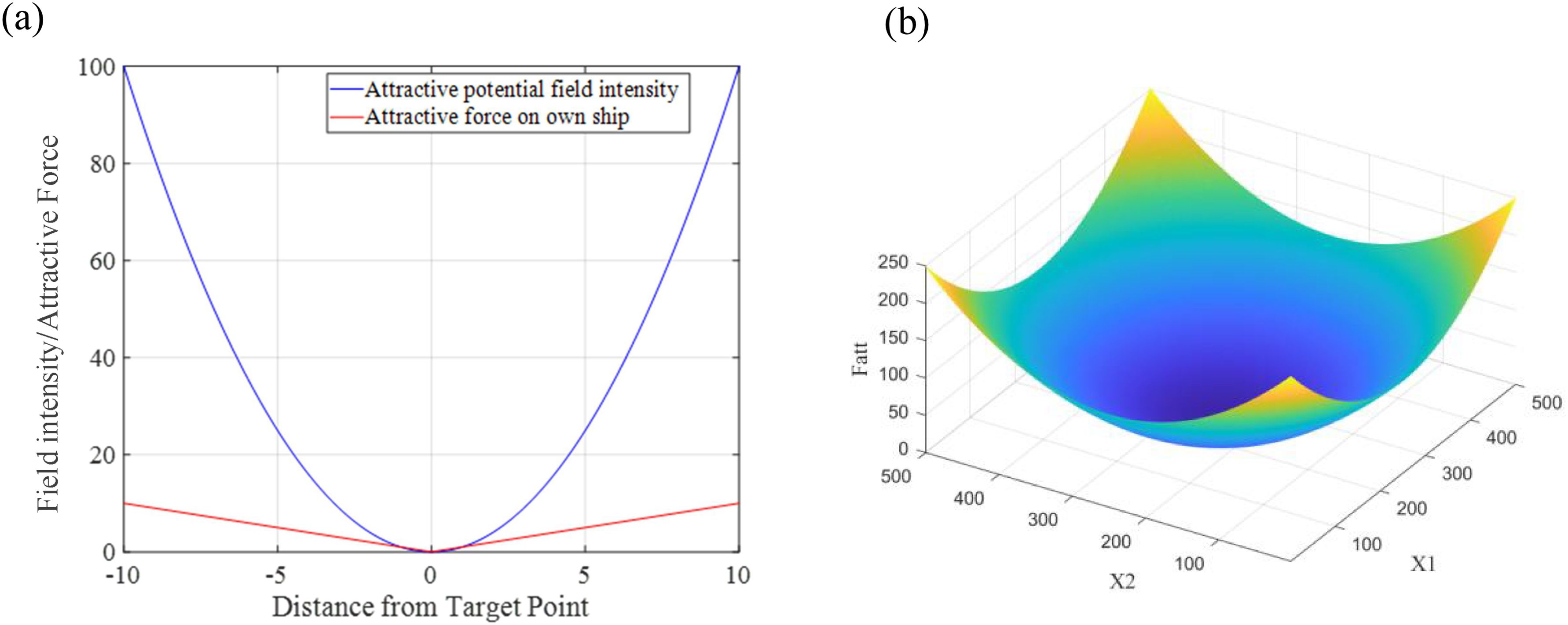
Figure 1. The attractive potential field. (A) The field gradient change curve. (B) 3D plot of the field.

For an unreachable target, this paper segments the traditional APF functions based on its structure, turning the potential field at the position near the target point from a quadratic function type to a cone type, so that the own ship is subject to a sufficiently large attractive force when it is near the target point and can reach the target point, and the improved attractive potential field function is as Equation 7:

$\begin{array}{ll}{U}_{att}(q)=\{\begin{array}{c}ϵ\sqrt{{\rho }^2(q,q_g)}-\mu ,\rho (q,q_g)<{\rho }_1\\ \frac{1}{2}ϵ{\rho }^2(q,q_g),\rho (q,q_g)\ge {\rho }_1\end{array}& (7)\end{array}$

where μ is a constant. The improved attractive potential field classifies the position of the own ship, and if the distance from the target point is greater than the set distance ρ₁, the attractive potential field is calculated according to the traditional APF function; if the distance from the target point is less than or equal to ρ₁, the attractive potential field is calculated according to the conic surface formula with the constant μ to make the difference. The attractive force at this point is shown in Equation 8:

$\begin{array}{ll}{F}_{att}(q)=-\nabla [U_{att}(q)]=-\frac{\partial U_{att}(q)}{\partial \rho }=\{\begin{array}{c}-ϵ,\rho (q,q_g)<{\rho }_1\\ -ϵ\rho (q,q_g)e_{\tau },\rho (q,q_g)\ge {\rho }_1\end{array}& (8)\end{array}$

Compared to the traditional APF, the improved algorithm has the same attraction at distances greater than ρ₁ from the target point, while the region within ρ₁ from the target point is subject to a stronger attraction, thus enabling the own ship to reach the target point by overcoming the target inaccessibility problem generated by obstacle repulsion (Figure 2).

Figure 2

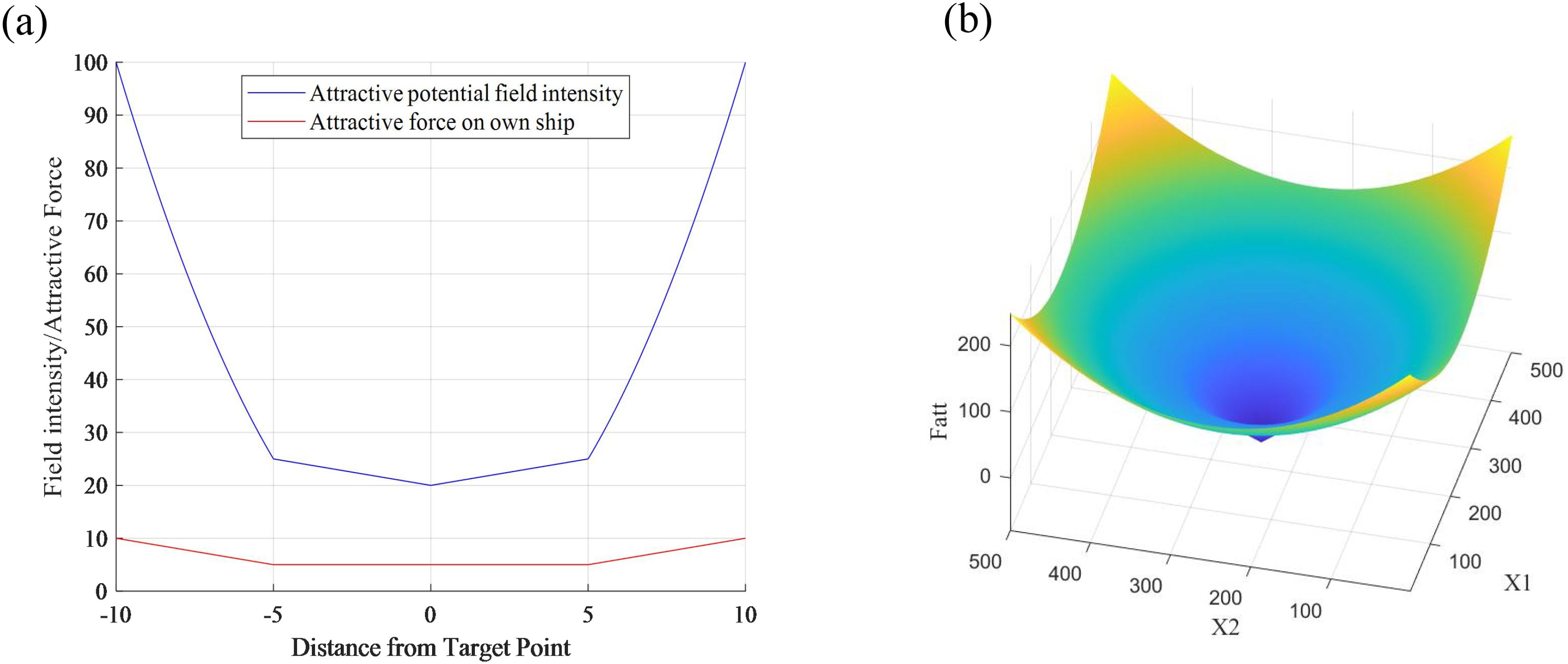
Figure 2. The improved attractive potential field. (A) The gradient change curve. (B) 3D plot of the field.

Furthermore, the distance between the own ship and the target point is introduced into the repulsive function, so that the repulsive force of the obstacle on the own ship changes with the distance from the own ship to the target point. Specifically, when the own ship is far from the target point, the repulsive force on the own ship increases compared with the traditional function, to offset the influence of the attractive force and overcome the path interference problem to avoid the obstacle. When approaching the target point, the repulsive force of the obstacle gradually decreases, and the own ship can be guided to the target point to complete the navigation task with the attractive potential field at the same time, which further overcomes the influence of the problem of an unreachable target. The mathematical expression of the improved repulsive potential field function is as Equation 9:

$\begin{array}{ll}{U}_{rep}(q)=\{\begin{array}{c}\frac{1}{2}\eta {(\frac{1}{\rho (q,q_{ob})}-\frac{1}{{\rho }_0})}^2{\rho }^2(q,q_g),\rho (q,q_{ob})\le {\rho }_0\\ 0,\rho (q,q_{ob})>{\rho }_0\end{array}& (9)\end{array}$

The repulsive force F_rep(q) at this point is divided into two parts, F_r1(q) and F_r2(q), as shown in the Equations 10–12:

$\begin{array}{ll}{F}_{rep}(q)=-\nabla [U_{rep}(q)]=-\frac{\partial U_{rep}(q)}{\partial \rho }=\{\begin{array}{c}{F}_{r1}(q)+F_{r2}(q),\rho (q,q_{ob})\le {\rho }_0\\ 0,\rho (q,q_{ob})>{\rho }_0\end{array}& (10)\end{array}$

$\begin{array}{ll}{F}_{r1}(q)=\eta (\frac{1}{\rho (q,q_{ob})}-\frac{1}{{\rho }_0})\frac{{\rho }^2(q,q_g)}{{\rho }^2(q,q_{ob})}{e}_{\tau }& (11)\end{array}$

$\begin{array}{ll}{F}_{r2}(q)=\eta {(\frac{1}{\rho (q,q_{ob})}-\frac{1}{{\rho }_0})}^2\rho (q,q_g)e_{\tau }& (12)\end{array}$

The direction of vector F_r1(q) is pointing from the obstacle to the own ship, and the direction of vector F_r2(q) is pointing from the own ship to the target point, as shown in Figure 3.

Figure 3

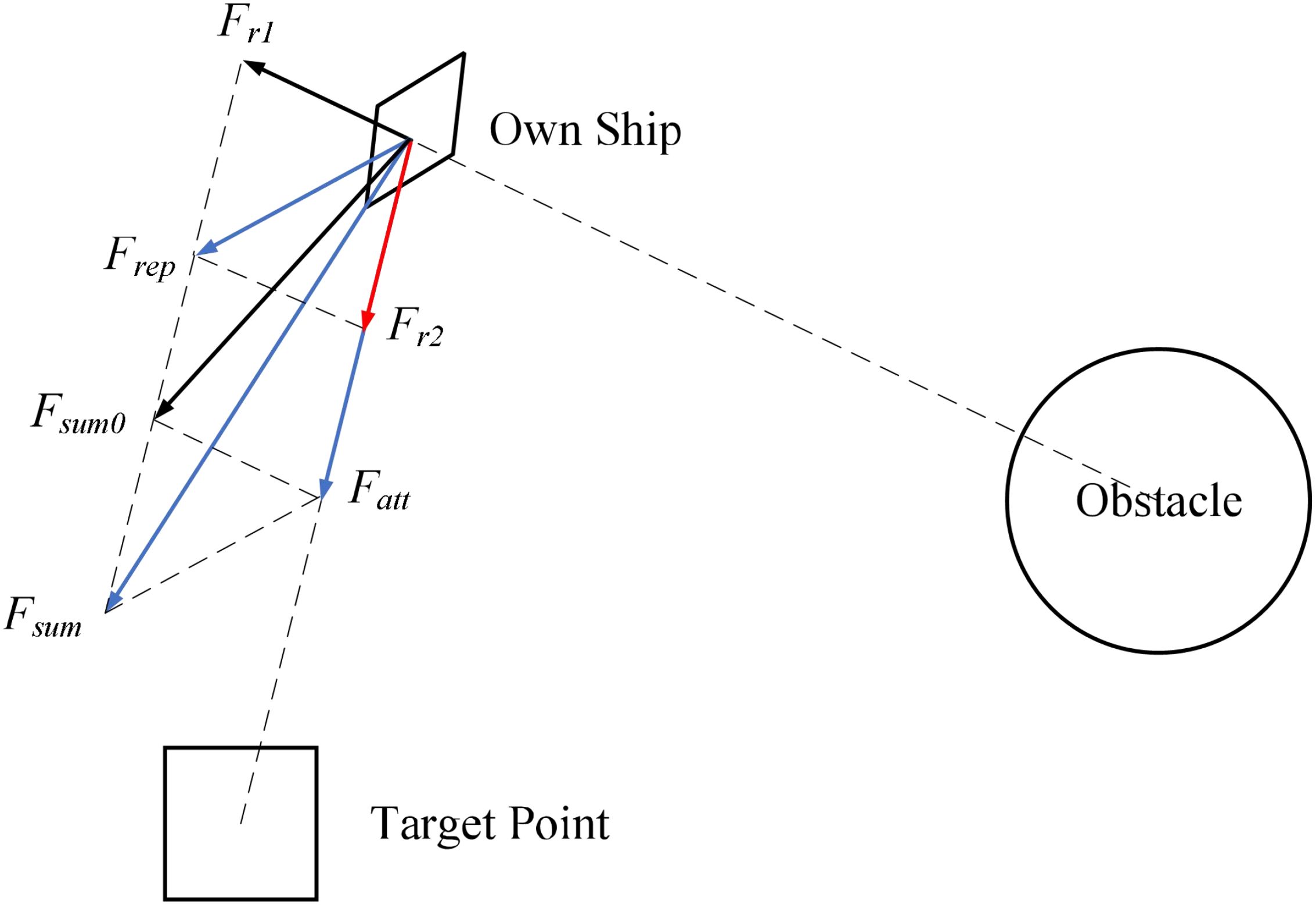
Figure 3. The improved-APF for the repulsive force on the own ship.

Compared with the combined force F_sum0 of the traditional APF, the improved combined force F_sum1 of the own ship tends to the target point more and thus overcomes the target inaccessibility problem.

2.2.2 Dynamic window approach

When using the traditional APF for collision avoidance, the two factors of the obstacles’ repulsion and the target point’s attraction are usually used as the contributions of the potential fields, respectively, and their superposition is calculated to enable the own ship to avoid obstacles while moving toward the target point. However, due to the certain competition between the attractive and repulsive fields, the own ship may experience path oscillations when passing through narrow areas between multiple obstacles, leading to unstable actions and even falling into the local optimum, which in turn affects the performance and efficiency of the own ship during navigation.

To solve this problem, this paper introduces the idea of DWA (Thomas et al., 2008) fused into the APF, which can achieve local dynamic collision avoidance and smooth path generation at the same time. DWA is a classical local path planning algorithm. The process is divided into two main parts.

(1) Calculation of the velocity space. Considering the actual motion constraints, a velocity range can be calculated as expressed in Equation 13:

$\begin{array}{ll}V=\left\{(v,\omega )|v_1<v<v_2,{\omega }_1<\omega <{\omega }_2\right\}& (13)\end{array}$

where v₁ = v₀ - at, v₂ = v₀ + at, ω₁ = ω₀ - t, and ω₂ = ω₀ + t. t is the set prediction time period, which indicates the velocity or angular velocity after moment t.

This range is determined by a variety of factors, including velocity, acceleration limits, rotation angle, and angular acceleration limits, in addition to the stopping distance limit that can stop the own ship in time before the collision is considered.

(2) Evaluation of the velocity space (v, ω). According to the given evaluation formula, each group in the velocity space is evaluated, and then the best set of velocities is selected as the current speed.

Through various parameters of ship motion that are artificially set before the experiment, such as maximum speed, acceleration, and maximum angular speed, which are used to update the dynamic window, the updated positional information is adjusted by calculating the speed, acceleration, angular speed, and other factors in the current state of the own ship to avoid the own ship making violent steering movements and make the own ship act along a trajectory more in line with the actual operation and more smoothly and naturally.

Regarding the evaluation formula, this section uses the calculated dynamic velocity window as a constraint to fuse into the position update function of the artificial potential field, and constrains the dynamic window by the gradient descent direction of the established artificial potential field to reduce the velocity search space, so that the own ship selects a position that conforms to the gradient change of the potential field and satisfies the mathematical model of ship motion to achieve a collision avoidance operation that is more in line with the actual situation. The ship’s optimal positional information is then screened and position velocity updated according to the evaluation formula, and the calculation of the own ship’s positional information set is shown as Equation 14:

$\begin{array}{ll}X(v_i,{\omega }_i)=[\begin{array}{c}x\text{'}\\ y\text{'}\\ \theta \text{'}\end{array}]=\{\begin{array}{c}[\begin{array}{c}x-\frac{v_i}{{\omega }_i}\text{sin}\theta +\frac{v_i}{{\omega }_i}\sin (\theta +{\omega }_{i}t)\\ y+\frac{v_i}{{\omega }_i}\text{cos}\theta -\frac{v_i}{{\omega }_i}\cos (\theta +{\omega }_{i}t)\\ \theta +\omega t\end{array}]({\omega }_i\ne 0)\\ [\begin{array}{c}x+v_i\cos \theta t\\ y+v_i\sin \theta t\\ \theta \end{array}]({\omega }_i=0)\end{array}& (14)\end{array}$

After obtaining the set of positional information and filtering it according to the evaluation formula, the evaluation formula consists of four main parts, which are expressed mathematically as follows:

i. Heading. Calculate all possible positional information in the range of velocity resolution by prediction time t, and calculate the difference between its corresponding angle theta and the direction of the combined force applied to the own ship in the constructed artificial potential field, the smaller the difference, the higher the rating. The formula is shown as Equation 15:

$\begin{array}{ll}heading(v_i,{\omega }_i)=180-\left|theta(q,q_{APF})-{\theta }^{\prime }\right|& (15)\end{array}$

ii. Obstacles. Static obstacles must be considered in order to verify the collision avoidance effect in complex water areas. For other dynamic ships, it is impossible to avoid them with global path planning, so the distance between the own ship and other dynamic ships is calculated after each update of the ship’s position and is determined by the ship domain set in section 3 of this paper. For the other ship outside the own ship’s domain, the farther the distance, the higher the score, while setting the upper limit of the score to avoid the excessive weight of the evaluation function. The formula is shown as Equation 16:

$\begin{array}{ll}distance(v_i,{\omega }_i)=\{\begin{array}{c}\text{min}[\rho (q,q_{ob})],distance<{\rho }_1\\ {\rho }_1,distance>{\rho }_1\end{array}& (16)\end{array}$

where ρ is the upper limit of the score set, which takes effect when the own ship is in open water and there are no dynamic other ships around, to ensure that the algorithm does not fall into the local optimum.

iii. Speed. To ensure navigation efficiency, the speed should be as high as possible, so it is expressed directly in absolute value. The formula is shown as Equation 17:

$\begin{array}{ll}velocity(v_i,{\omega }_i)=\left|v_i\right|& (17)\end{array}$

iv. Stopping distance. If the distance between the own ship and other ships is within the own ship’s domain or collision cannot be avoided then the cycle is jumped out and recalculated, which is equivalent to the emergency braking operation.

The final evaluation function is mathematically expressed as the weighted average of the above three components. The formula is shown as Equation 18:

$\begin{array}{ll}G(v_i,{\omega }_i)=\delta ·heading(v_i,{\omega }_i)+\beta ·distance(v_i,{\omega }_i)+\gamma ·velocity(v_i,{\omega }_i)& (18)\end{array}$

where the value of δ, β, γ can be adjusted according to the demand. In addition, the traditional dynamic collision avoidance method can usually only use the method of changing direction to avoid obstacles during collision avoidance, and although this method is simple and easy to implement, the efficiency of collision avoidance is limited and the maneuvering performance of the own ship cannot be fully utilized. However, the algorithm characteristics of the dynamic window method can traverse all situations with a set speed resolution within the eligible condition and can consider deceleration while steering, thus avoiding collisions to the greatest extent, and improving the efficiency and accuracy of collision avoidance.

3 Dynamic collision avoidance preconditions

3.1 Encounter situation division and the own ship’s action

A vessel encounter situation refers to two or more vessels encountering each other in navigation and needing to avoid collision by mutual communication and coordination. According to Rules 13, 14, and 15 of COLREGS, the meeting of ships in mutual encounters can be divided into the following three situations as shown in Figure 4.

Figure 4

Figure 4. A schematic diagram for identifying the encounter situation.

Overtaking: A vessel shall be deemed to be overtaking when coming up with another vessel from a direction more than 22.5 degrees abaft her beam, that is, in such a position with reference to the vessel she is overtaking, that at night she would be able to see only the stern light of that vessel but neither of her sidelights.

Head-on: Such a situation shall be deemed to exist when a vessel sees the other ahead or nearly ahead and by night, she could see the masthead lights of the other in a line or nearly in a line and/or both sidelights and by day she observes the corresponding aspect of the other vessel.

Crossing: When two power-driven vessels are crossing to involve risk of collision, the vessel which has the other on her own starboard side shall keep out of the way and shall, if the circumstances of the case admit, avoid crossing ahead of the other vessel.

In addition, Rule 19 of COLREGS lists an encounter when visibility is poor as a separate situation, and provides for collision avoidance actions at this time, which should be avoided as far as possible as follows:

i. An alteration of course to port for a vessel forward of the beam, other than for a vessel being overtaken;

ii. an alteration of course towards a vessel abeam or abaft the beam.

Figure 5 shows more specific collision avoidance strategies in three encounter situations, where the black solid arrows indicate the respective ship’s heading and the red dashed arrows indicate the direction of steering that should be selected when the corresponding ship takes collision avoidance action.

Figure 5

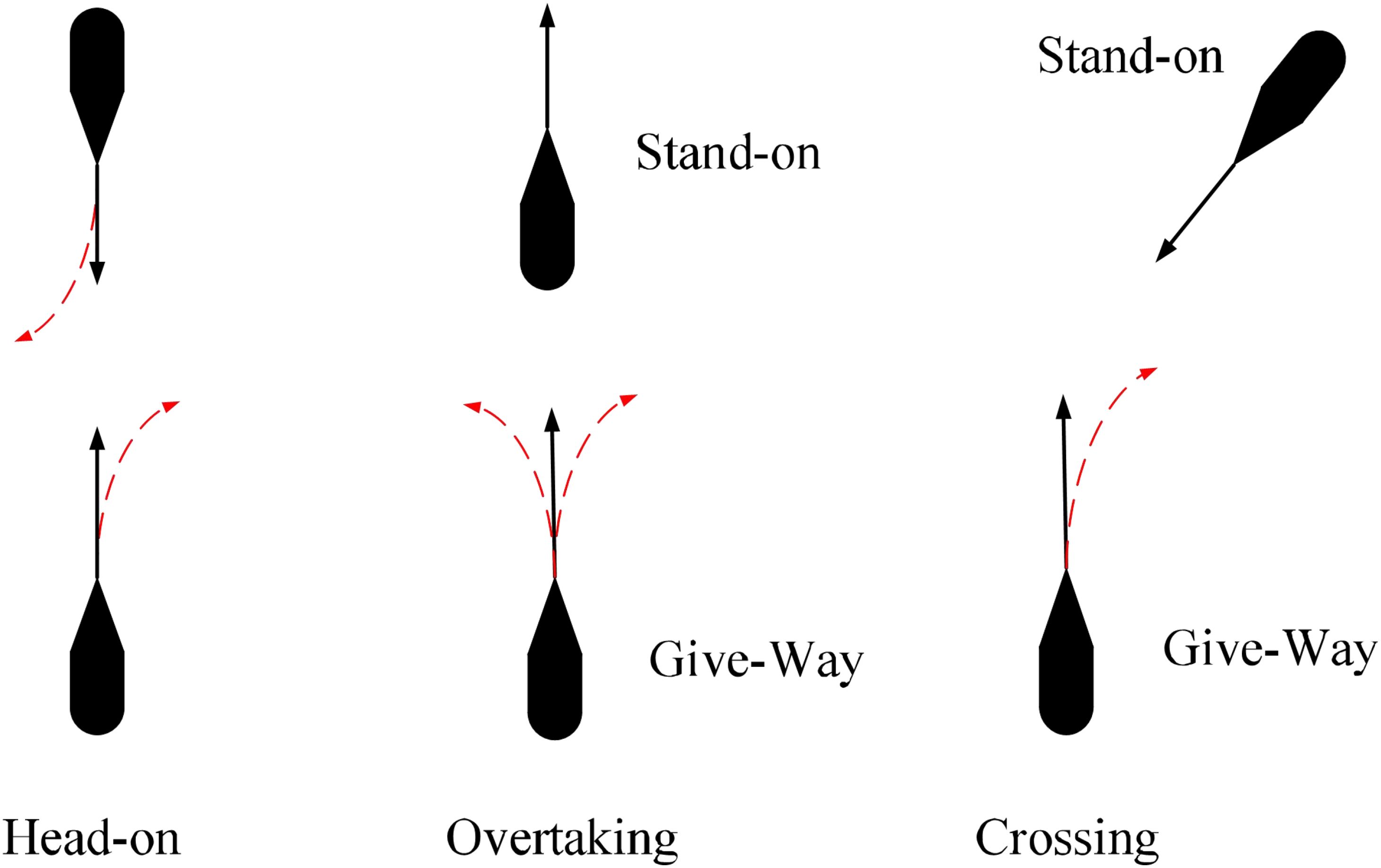
Figure 5. A schematic diagram of three encounter situations.

In head-on, overtaking, and crossing situations, according to the requirements of Rule 8 of COLREGS, every vessel is directed to keep out of the way of another vessel shall, so far as possible, and take early and substantial action to keep well clear, that is, if the circumstances of the case admit, the action of collision avoidance should be positive, made in ample time and with due regard to the observance of good seamanship, be large enough to be readily apparent to another vessel observing visually or by radar. In addition, a succession of small alterations of course and/or speed should be avoided, and steering alone may be the most effective action to avoid a close-quarters situation, and it is required that such an action is in good time and substantial and does not result in another close-quarters situation. Finally, by giving way to stand-on vessel to take collision avoidance action. The action taken to avoid collision with another vessel shall be such as to result in passing at a safe distance. Due to the complex and changing environment at sea, the effectiveness of the action shall be carefully checked until the other vessel is finally past and clear.

3.2 Collision risk assessment

Rule 7 of COLREGS is “Risk of Collision”, but there is no clear definition or description of it. Risk of collision is a possibility, which can be generally understood as a potential collision possibility and all unsafe factors between two ships or between a ship and its surroundings. The assessment of collision risk is difficult to define by quantitative methods\ and the same effect can be achieved by considering a distance appropriate to the prevailing circumstances and conditions (required by Rule 6 of COLREGS) from the opposite side, thus giving birth to the concept of ship domain (Arimura et al., 1994).

The ship domain can be roughly classified into three categories: determined empirically, experts` knowledge, and analytical. However, each method has its limitations due to the complex factors that need to be considered in constructing a ship domain model. Considering the different safety distances observed in different directions, this section adopts the concept of quadratic ship domain as the basis for collision hazard assessment. The quaternion ship domain considers the requirements of the COLREGS, good seamanship, ship maneuverability, and ship length and speed, making it more suitable for collision avoidance at sea.

The Quaternion Ship Domain (QSD) consists of four defined elements: Q (i.e., R_f, R_a, R_p, and R_s), with R_f and R_a denoting the own ship’s fore and aft respectively, R_p and R_s denoting the own ship’s port and starboard respectively. The QSD is composed of the region defined by the closed curve connecting these four elements and the interior region can be described as Equation 19:

$\begin{array}{ll}{f}_{\tau }(x,y;Q)={(\frac{2x}{(1+\text{sgn}x)R_f-(1-\text{sgn}x)R_a})}^{\tau }+{(\frac{2y}{(1+\text{sgn}x)R_s-(1-\text{sgn}x)R_p})}^{\tau }& (19)\end{array}$

where τ is a parameter that controls the shape of the QSD. The value of τ is typically set to 1 or 2 depending on the desired level of detail for the QSD’s shape. The sgn function is defined as the signum function, which is used to determine the sign of a variable. It is defined mathematically as Equation 20:

$\begin{array}{ll}\text{sgn}(x)=\{\begin{array}{c}1,x\ge 0\\ -1,x<0\end{array}& (20)\end{array}$

This function is used in the QSD formula to calculate the contribution of the forward, aft, port, and starboard regions based on the relative position of the ship. In the context of blocking area estimation, the lateral and longitudinal radii of the QSD are calculated, which are important for determining the extent of the ship’s domain. These radii are defined by Equation 21:

$\begin{array}{ll}\{\begin{array}{c}\begin{array}{c}{R}_f=(1+1.34\sqrt{k_{AD}^2+{(\frac{k_{DT}}{2})}^2})L\\ R_a=(1+0.67\sqrt{k_{AD}^2+{(\frac{k_{DT}}{2})}^2})L\end{array}\\ \begin{array}{c}{R}_s=(0.2+k_{AD})L\\ R_p=(0.2+0.75k_{AD})L\end{array}\end{array}& (21)\end{array}$

where L is the own ship’s length and k_AD is the gain coefficient of the own ship’s cyclotron distance A_D, representing the own ship’s position relative to its initial point. Furthermore, k_DT is the gain coefficient of the cyclotron initial diameter D_T, representing the own ship’s initial speed or other related parameters. These two coefficients can be calculated from the own ship’s captain and the own ship’s cyclotron test parameters, and the equations are as Equation 22 (Kijima and Furukawa, 2003):

$\begin{array}{ll}\{\begin{array}{c}{k}_{AD}=\frac{A_D}{L}={10}^{0.3591\text{lg}(v_0)+0.0952}\\ k_{DT}=\frac{D_T}{L}={10}^{0.5441\text{lg}(v_0)-0.0795}\end{array}& (22)\end{array}$

where v₀ represents the speed of the own ship. From equation (22), the gain coefficient shows a positive relationship with the own ship speed and the quaternion number with the ship length. Correspondingly, the size of the formed ship domain increases with an increase in the ship scale and speed. τ is taken as 1 and 2 for the quaternion ship domain model, as shown in Figure 6, and the value of τ for the ship domain model in this paper is taken as 2.

Figure 6

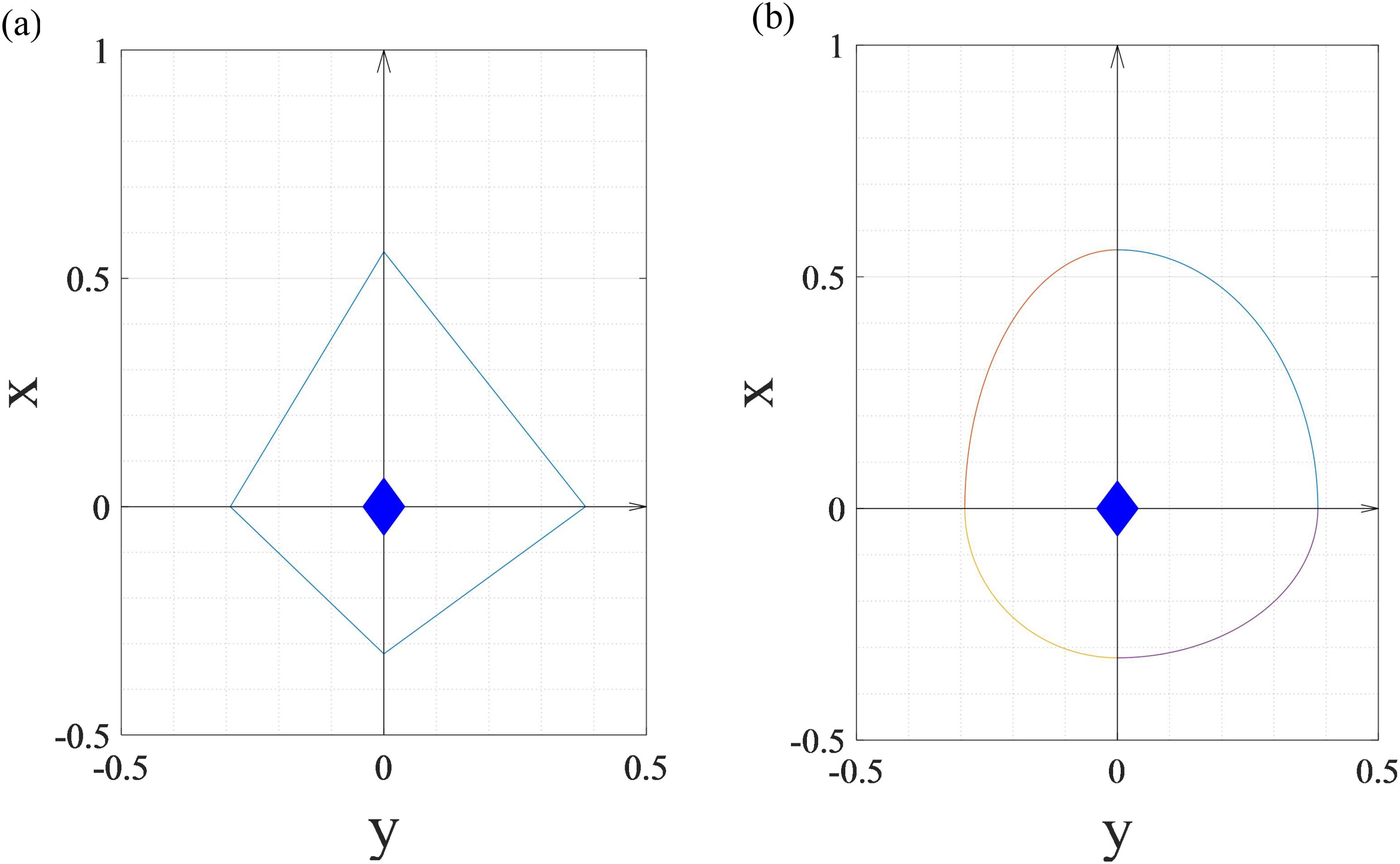
Figure 6. Quaternion ship domain model when τ equals 1 and 2. (A) Quadratic ship domain shape when τ = 1. (B) Quadratic ship domain shape when τ = 2.

Hereto, all the necessary information about the improved APF model proposed in this paper is introduced. Figure 7 is a complete structural block diagram of the model.

Figure 7

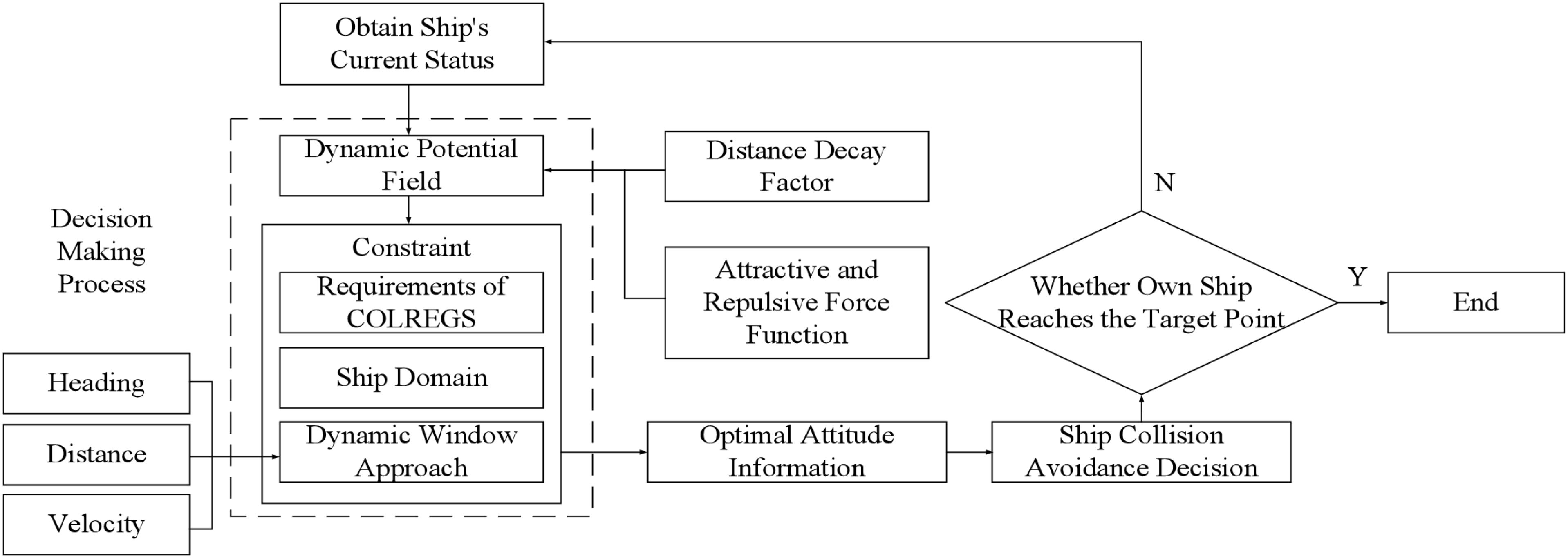
Figure 7. The structural block diagram of the improved-APF model.

As in the block diagram in Figure 7, the model initiates by computing the attractive and repulsive forces based on the ship’s current position, target location, and surrounding obstacles. These forces are then integrated to determine the overall movement direction. Following this, the dynamic window is established to define the feasible velocity (v) and angular velocity ranges (ω), taking into account the ship’s dynamic constraints such as maximum speed and acceleration limits. Within this window, a set of candidate velocity commands is generated and evaluated against criteria including alignment with the desired heading, distance, and velocity (navigation efficiency). The optimal velocity command is selected to update the ship’s position, and the process iterates until the target is reached. The subsequent pseudo code encapsulates these procedural steps, providing a clear and structured implementation framework for the algorithm (See Algorithm 1).

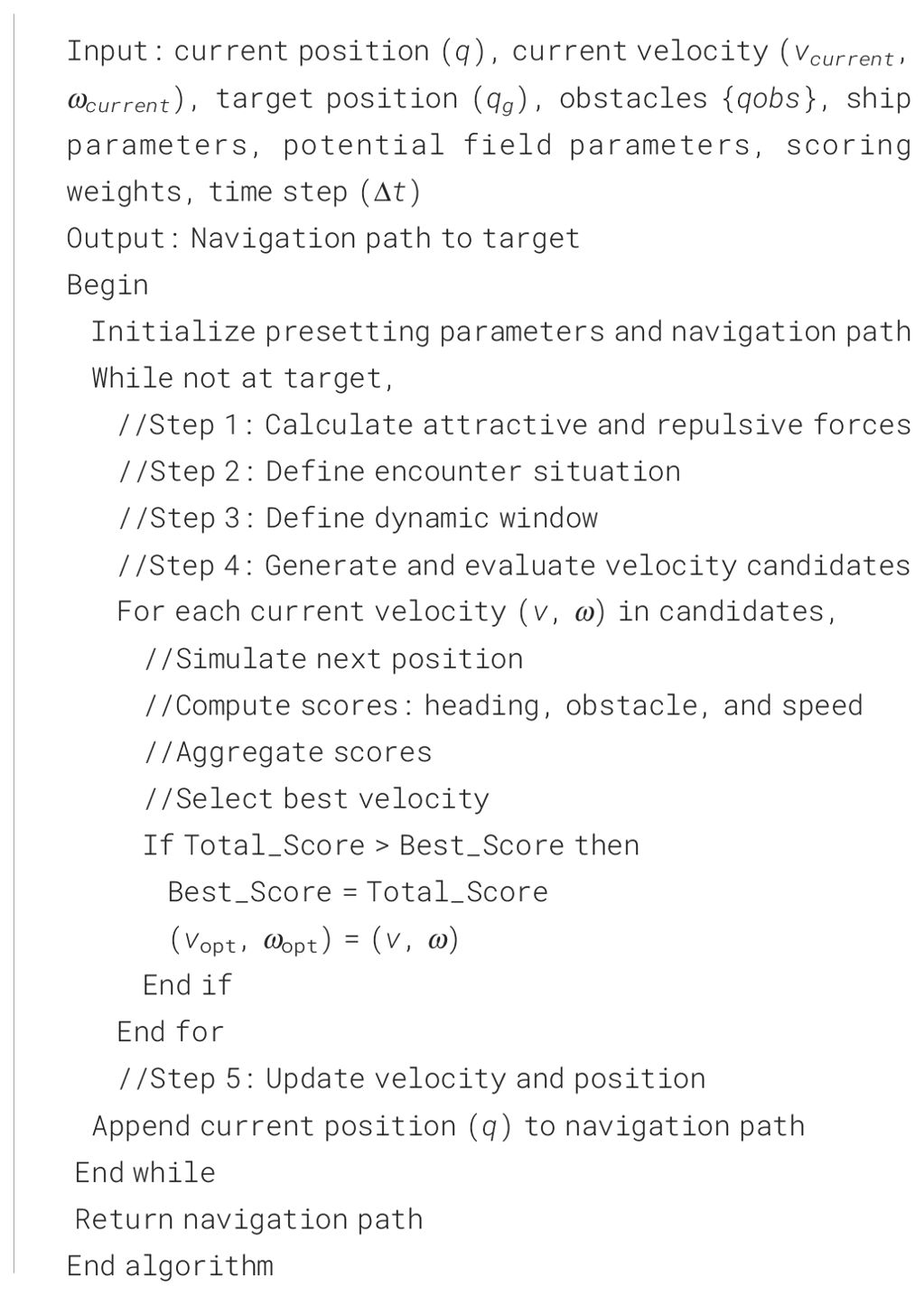
Algorithm 1. Algorithm process of the improved-APF.

4 Simulation experiments

In order to verify the generalization ability of the improved-APF algorithm proposed in this paper under different avoidance requirements, simulation experiments were conducted on the performance of the improved-APF algorithm in avoiding other dynamic ships in different scenarios.

The improved-APF incorporates several critical parameters that influence its performance, including the weighting coefficients (δ, β, and γ) for the evaluation of the own ship’s heading, distance from obstacles, and velocity, respectively. These parameters are crucial in determining the balance between safety and efficiency in collision avoidance. The selection of these coefficients was based on a combination of theoretical understanding and practical experimentation. Specifically, the values of δ, β, and γ were chosen to prioritize heading control, obstacle distance, and velocity under typical operational conditions. Heading control (δ) is more critical in real-world navigation scenarios where maintaining course stability is essential, while the proximity to obstacles (β) and velocity (γ) are secondary to ensuring safe and efficient maneuvering.

Additionally, the values of the speed and steering parameters, such as the maximum speed and turning rate, were derived from practical ship operational limits to ensure realistic and feasible performance under typical navigation conditions. In order to determine the weighting coefficients (δ, β, and γ) of the evaluation function, a simple control test is shown in Figure 8.

Figure 8

Figure 8. The simple control test map.

The map was set up as a vector map of a single obstacle of the same size as the formal simulation trials, as shown in Figure 8. The coordinates of the starting point and the target point are (0, 0) and (220, 300) respectively. Furthermore, the ship type parameters and ship motion parameters used in this section are taken from the practice ship ‘YUPENG’ of Dalian Maritime University in conditions for the right rotation back 35° real ship experiment (Yang et al., 2017), and some of them were selected for the simulation experiments of the improved-APF. Details are shown in Table 1:

Table 1

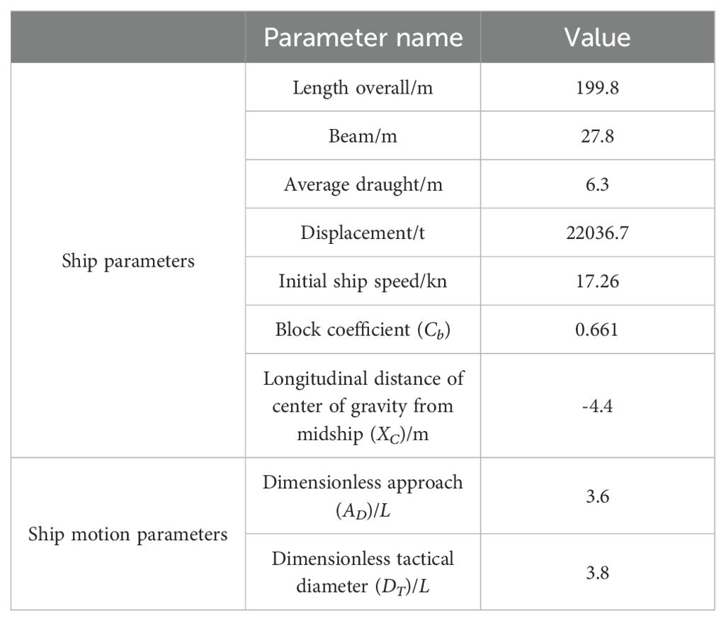
Table 1. The parameters of M/V YUPENG.

By setting different weighting coefficients, the path length (PL), iteration (I) and closest distance to the obstacle (D_C) were evaluated as quantitative indicators. The complete testing process is too long to be shown in full, and several representative cases (based on 0.2/0.5/0.8) were selected to be analyzed and illustrated in Table 2, ∞ means the algorithm fails to complete the task, that is, OS collides with obstacles or fails to reach the target point, which will cause the values of PL and I to approach infinity.

Table 2

Table 2. The test results under different weighting coefficients.

In Table 2, there are three types of coefficient sets named Sequence, Peak, and Valley, respectively. They represent the whole shape of the coefficient sets in an equidistant series or two small and one large, or two large and one small. The test results for numbers 3, 5, 6, 9, and 11 were more favorable. Their common pattern was δ > β, while β< γ, i.e., the heading was weighted more than the distance. For this setting, the algorithm generates a relatively short path, the iteration efficiency is high and can maintain a certain safe distance from the obstacles. On this basis, the final program selected was No. 3(δ: 0.5, β: 0.2, γ: 0.8).

In addition to the own ship type parameters, the parameters of the improved-APF algorithm itself need to be set, including the corresponding weights of the evaluation function, the upper limit of the algorithm iterations (E_max: 50000), the upper limit of the velocity (V_max/kn: 12), and turning speed (ω_max/rad·s^-1: 0.52) of the own ship, and the resolution corresponding to the velocity (V_Res: 0.1) and turning speed (ω_Res: 0.012) in the simulation experiment, which mean the minimum intervals during changes in the ship’s velocity and turning speed.

As a basis for evaluating the collision risk, the range of the quadratic ship domain in the case of different ship speeds also changes. In order to judge the effect of the simulation test more accurately, this paper calculated the distance of change of the QSD in the four directions of the own ship with different speeds by substituting the parameters in Table 1.

Table 3 shows that the QSD when the speed of the own ship was zero was a symmetrical ellipse, and when the own ship moves against the water, it changed to an irregular ellipse as shown in Figure 6B. With the increasing speed of the own ship, the judgment range of QSD increases, and its effective region is shown in Figure 9. Since the maximum ship speed was set to 12kn in the simulation experiment, the speed change range of the own ship in Table 3 was set to 0-12kn.

Table 3

Table 3. The quaternions at different ship speeds.

Figure 9

Figure 9. The distance change range of the QSD.

Figure 9 shows the QSD curves for ship speeds from 0kn to 12kn with a superimposed change of 0.1kn, and the increasing velocity in the range of QSD decreased as the ship speed increased and the domain stabilized. This situation is also consistent with reality, as ship speed does not increase indefinitely. It will lead to unnecessary collision avoidance maneuvers and thus reduce sailing efficiency if the ship domain is too large.

To more accurately replicate real-world conditions, this study overlayed a randomly generated composite potential field onto the simulated map environment as shown in Figure 10. This composite field comprises Gaussian vortices, constant potential fields, and random noise. The parameters and quantities of these components were randomly determined and vary progressively with each iteration, with the mixed potential field parameters being reset every 100 iterations. By introducing this background disturbance to better emulate the actual environment, the proposed method’s superiority and robustness were more comprehensively demonstrated, thereby enhancing the reliability and applicability of the experimental data.

Figure 10

Figure 10. The composite field. (A) 3D plot of the composite potential field. (B) Vector field representation of the negative gradient of the composite potential field.

The above is the static parameter setting process of the improved-APF. In order to test the avoidance ability of the model for dynamic obstacles (other ships) in local scenarios, four types of simulation test scenarios were set up, according to the head-on situation, overtaking situation, crossing situation, and multi-ship situation, and the map area was set as a square with a side length of 10 nautical miles and represented by a 500*500 vector map.

In the simulation situations set up according to the head-on situation, overtaking situation, and crossing situation, the path of the own ship (OS) generated by the improved-APF algorithm was set as a red line and the path of the target ship (TS) was set as a black line. In order to compare the situations more intuitively, a set of control tests was added to the same simulation scenario by applying the traditional APF algorithm, which only adds the improvement of the attractive repulsive potential field function based on the traditional APF and the constraints required by COLREGS to enable it to complete the collision avoidance task without falling into the local optimum and thus losing its role as a control, which is represented by the blue line.

(1)Situation 1: Head-on1

The initial information of the OS for Head-on1 is position (10, 10), course (045°), and speed (0kn); while the initial information of the TS for Head-on1 is position (490, 490), course (225°), and speed (8kn).

In this scenario, both the traditional-APF and the improved-APF turn to starboard, complying with the head-on requirements of COLREGS (i.e., Rule 14). However, the traditional APF’s resulting path features abrupt angular changes (Figure 11), demonstrating a lack of maneuverability considerations. This occurs because the traditional APF treats the obstacle (i.e., the target ship, TS) as a purely repulsive potential and does not account for the realistic turning constraints of a vessel, leading to sharp turns that deviate from actual ship-handling processes.

Figure 11

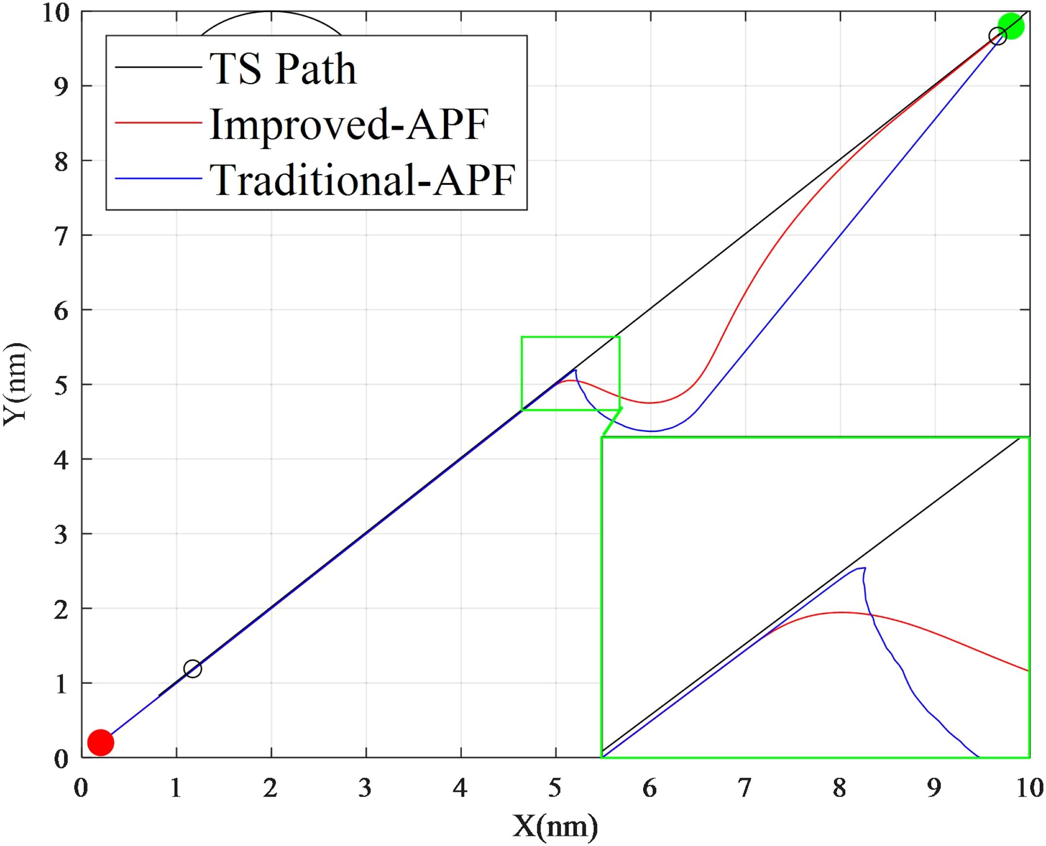
Figure 11. The comparison of simulation paths for Head-on1.

By contrast, the improved-APF produces a notably smoother path, initiating its starboard turn earlier and adjusting speed concurrently (around the 450th iteration in Figure 12). This two-pronged approach of steering and deceleration results in a more controlled encounter, ensuring a minimum passing distance of about 0.56 nm—which meets safety expectations for QSD. Additionally, the improved-APF re-accelerates and resumes its heading once past and clear of the TS, reflecting genuine navigational practices where ships return to their original course and speed after avoidance maneuvers.

Figure 12

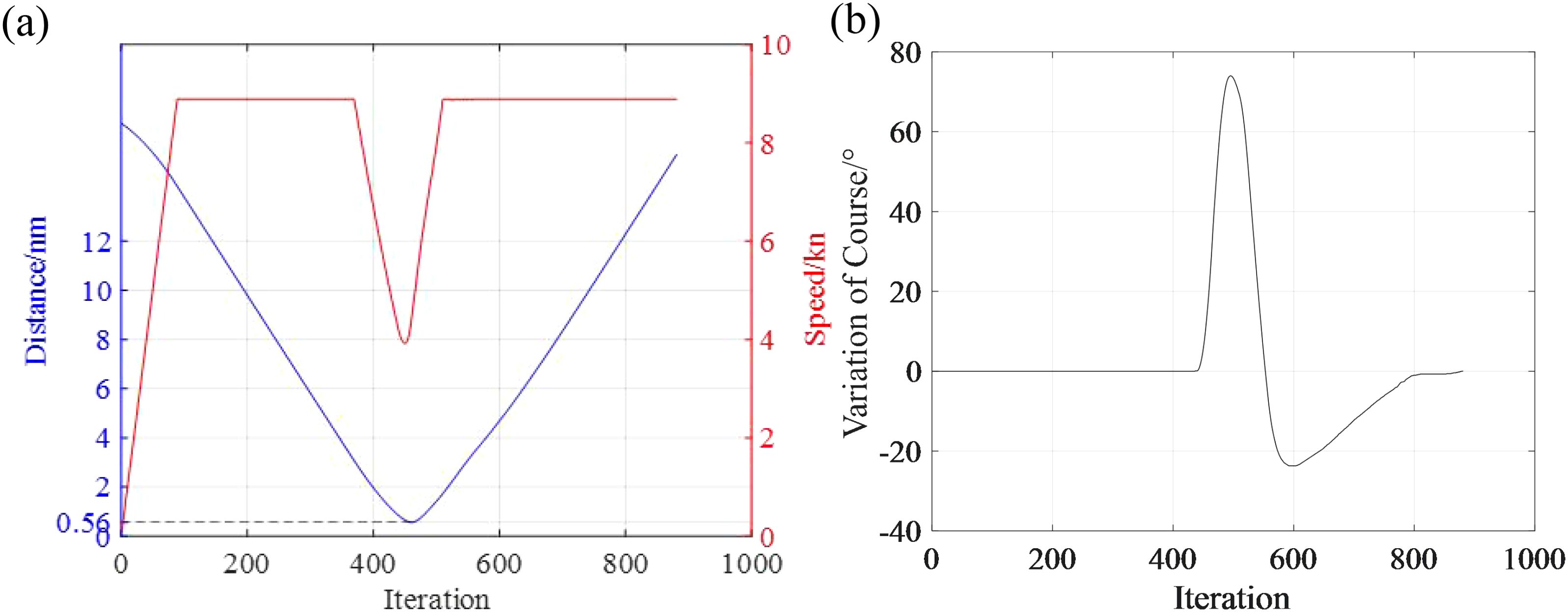
Figure 12. Situation 1 data change curve. (A) Distance between two ships and speed change of the OS. (B) Changes in the OS's course.

Such behavior underscores the key strength of incorporating dynamic constraints (e.g., bounded turning rates and variable speeds) into the path-planning algorithm. Not only does this produce maneuvers that better align with human navigation patterns, but it also enhances the vessel’s ability to plan avoidance actions more proactively. This early and smoother course alteration is particularly advantageous in reducing the collision risk when the encounter geometry rapidly changes.

(2)Situation 2: Head-on2

The initial information of the OS for Head-on2 is position (10, 10), course (045°), and speed (0kn); while the initial information of the TS for Head-on2 is position (500, 460), course (225°), and speed (6kn).

Unlike Situation 1, the OS and TS are crossing to involve risk of collision, starboard to starboard, in Situation 2 (Figure 13). If the steer starboard operation is still taken at this time, it will not only result in a longer path but also involve the risk of collision of passing the bow of TS when facing the simulation of the TS because it will not change its own course. Consequently, both the traditional APF and the improved-APF opt to turn to port, rather than starboard. This decision prevents the OS from attempting to pass starboard-to-starboard, which would pose a higher collision risk by bringing the OS closer to the TS’s bow. Thus, the improved-APF calculates that turning to starboard would produce a longer path and an increased likelihood of encountering TS’s forward sector. By turning to port, the OS achieves a safer, shorter route, demonstrating the algorithm’s capacity to adaptively interpret an encounter scenario when a standard COLREGS rule (Rule 14 for head-on) does not yield an optimal or safe solution.

Figure 13

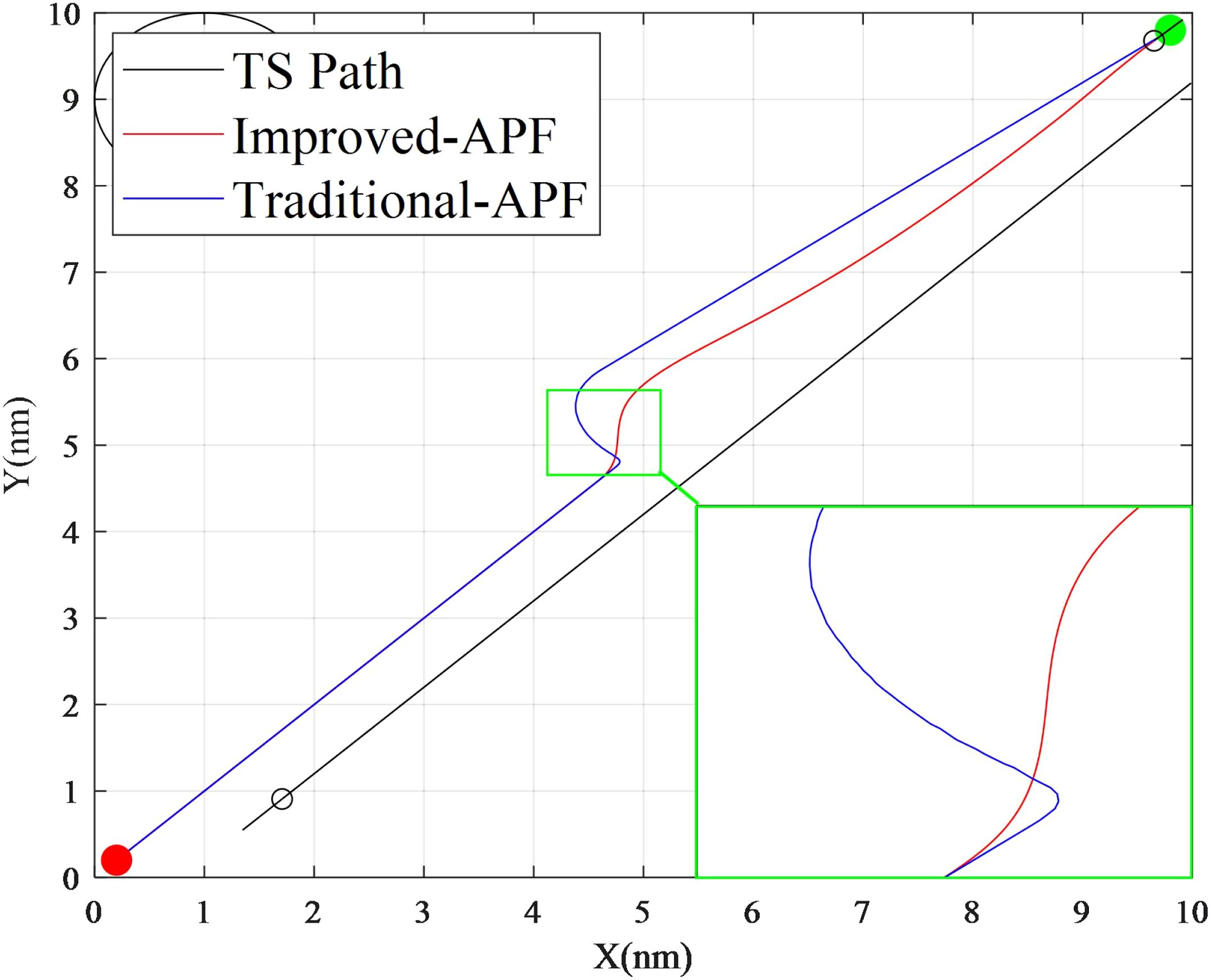
Figure 13. Comparison of simulation [aths for Head-on2.

Compared to the traditional APF, the improved-APF initiates this maneuver at an earlier stage, smoothly coupling the turn with a slight reduction in speed. This combined adjustment helps maintain a sufficient passing distance, preventing any near-bow crossings. Meanwhile, the traditional APF produces a more abrupt change, reflecting its purely repulsive potential calculation without factoring in maneuvering dynamics. The smoother profile of the improved-APF path again emphasizes the importance of accounting for vessel maneuverability and speed constraints. From a practical standpoint, this scenario highlights the algorithm’s flexibility in handling encounters that deviate from canonical head-on rules.

Figure 14 shows the speed and course change of the OS and the distance change between the OS and TS in Situation 2. The minimum distance in the avoidance process is 0.67nm, a safe distance according to maritime safety standards, confirming the algorithm’s capability in avoiding potential collisions.

Figure 14

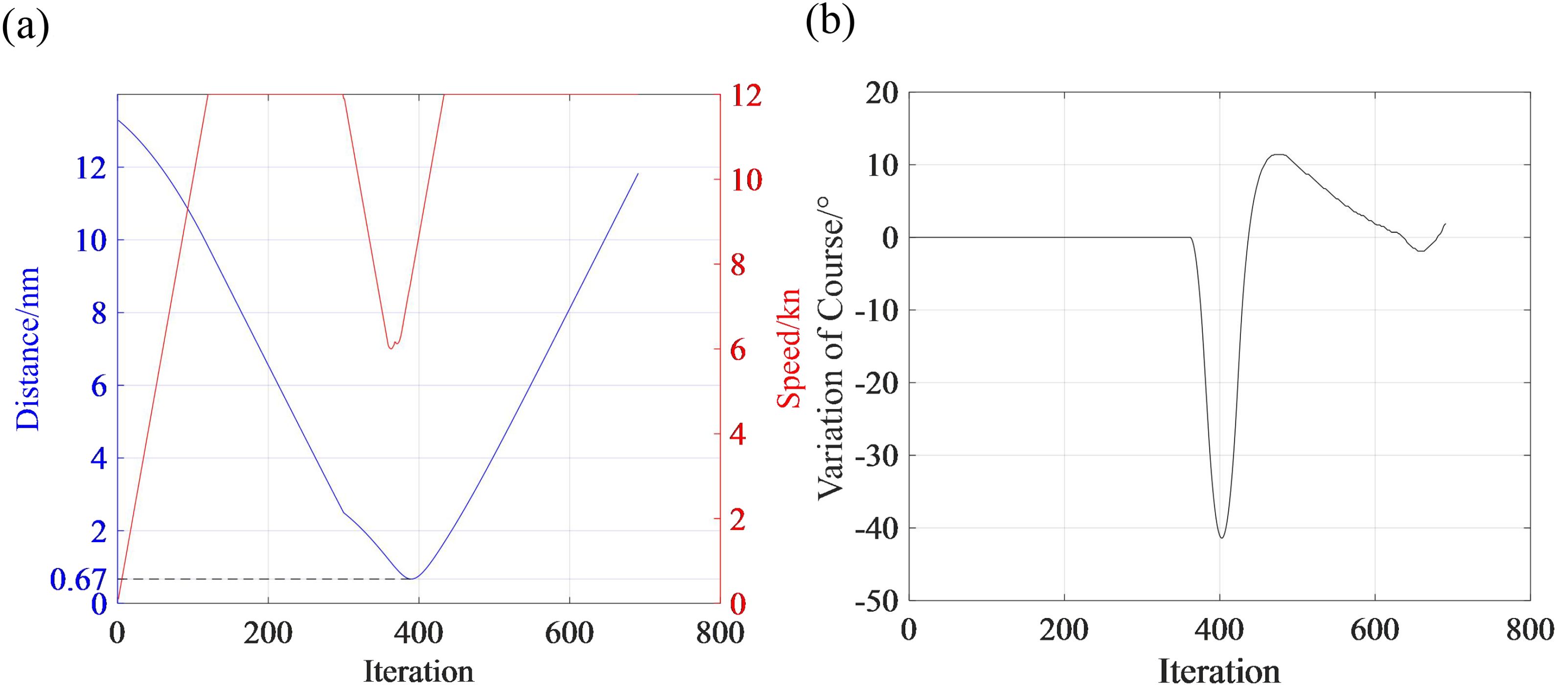
Figure 14. Situation 2 data change curve. (A) Distance between two ships and speed change of the OS. (B) Changes in the OS's course.

(3)Situation 3: Overtaking

The initial information of the OS for overtaking is position (10, 10), course (045°), and speed (0kn); while the initial information of the TS for overtaking is position (110, 100), course (045°), and speed (3kn).

The overtaking in Situation 3 (Figure 15) is set in a channel, requiring the OS to navigate as far as possible to the starboard, so the most suitable direction of overtaking is on the port side of the TS. According to the provisions of COLREGS for overtaking situations and quantitative analysis, the OS, as the give-way ship, should take effective avoidance action as early as possible. As can be seen from the path diagram, while both the improved-APF and the traditional APF algorithms generate a safe overtaking route, the traditional APF exhibits significant path oscillation during the process. This oscillation results in unnecessary changes in direction and course adjustments, which not only cause instability in the trajectory but also reduce the overall control precision and stability of the avoidance maneuver. In contrast, the improved-APF algorithm maintains a smoother and more stable path, making fewer abrupt course changes. It anticipates the overtaking maneuver with greater efficiency, applying the necessary adjustments earlier than the traditional APF. This results in a much more predictable and efficient overtaking trajectory. Additionally, the improved-APF algorithm integrates speed control during the overtaking process to reduce unnecessary acceleration or deceleration. This enhances the safety and stability of the maneuver, ensuring that the OS can smoothly navigate past the TS without overshooting or risking a collision, and the improved-APF algorithm is also adjusting its own course to do course-again operation after the TS is finally past and clear.

Figure 15

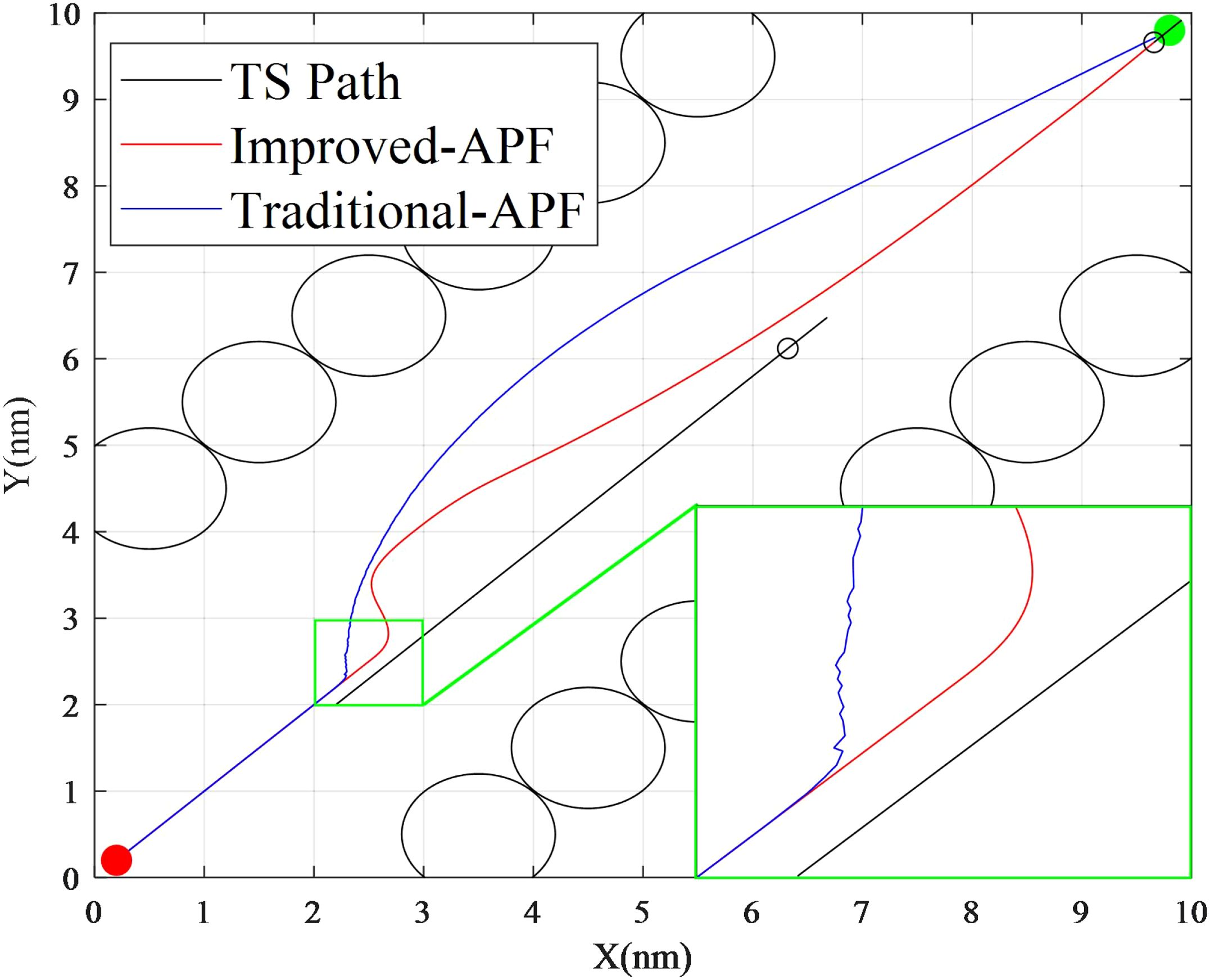
Figure 15. Comparison of the simulation paths for overtaking.

Figure 16 shows the process of speed and course variation of the OS and the process of inter-ship distance variation between the OS and TS in Situation 3 by the improved-APF. The minimum distance in the avoidance process is 0.84nm, a safe distance according to maritime safety standards, confirming the algorithm’s capability in avoiding potential collisions.

Figure 16

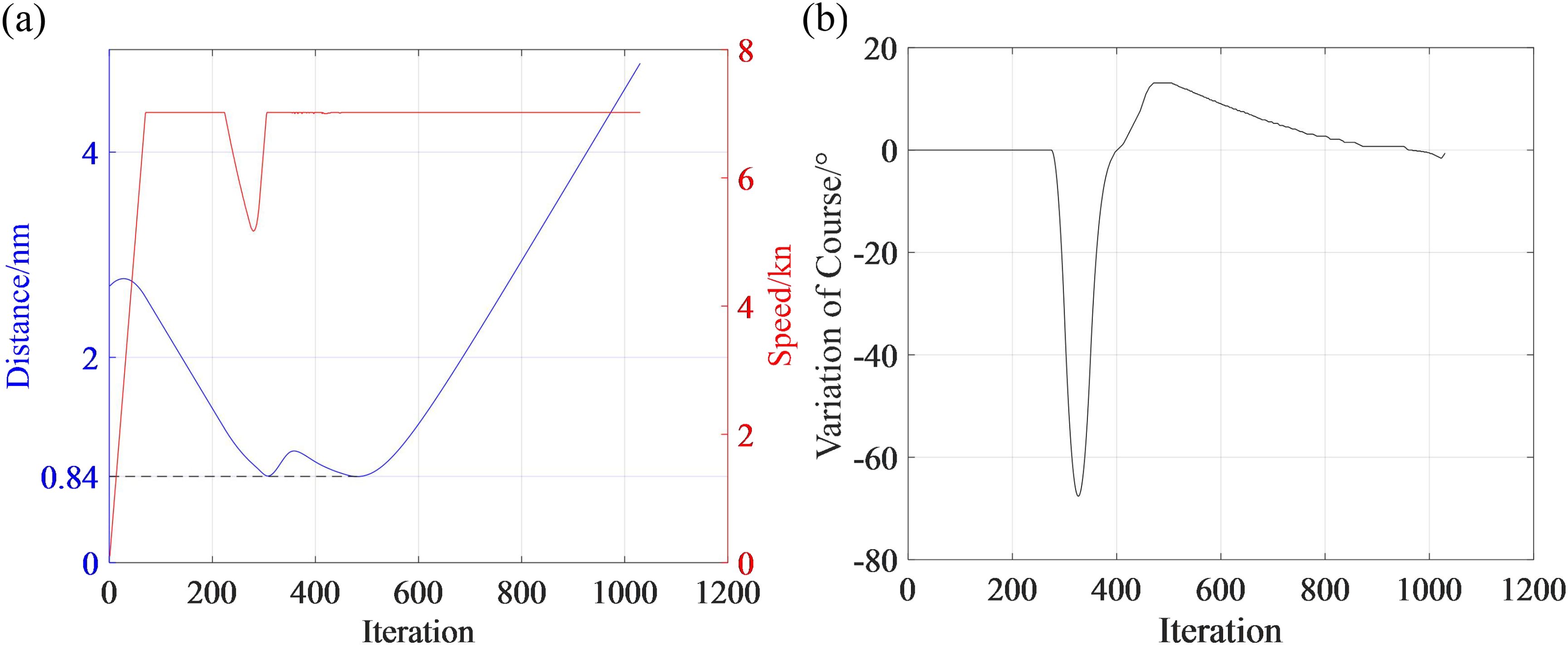
Figure 16. Situation 3 data change curve. (A) Distance between two ships and speed change of the OS. (B) Changes in the OS's course.

(4)Situation 4: Crossing1

The initial information of the OS for Crossing1 is position (10, 10), course (045°), and speed (0kn); while the initial information of the TS for Crossing1 is position (450, 310), course (270°), and speed (8kn).

In Situation 4 (Figure 17), according to the provisions of COLREGS for crossing situations and quantitative analysis, the OS should take effective avoidance action as the give-way ship at an early stage, and it can be seen from the collision avoidance path diagram that both the improved-APF and the traditional APF can take the avoidance measure of turning to starboard for the chase crossing situation, but it can be seen from the partially enlarged diagram in the lower right corner that the traditional APF has the path with a sharp angle and oscillation phenomenon that appeared in the first two sets of simulations. This sharp turn, which may seem valid in a simplified simulation, does not align with the actual maneuvering behavior of vessels in real-life scenarios. Vessels, in practice, rarely make sharp course changes due to physical limitations, such as turning radii and handling characteristics. In contrast, the improved-APF algorithm delivers a much smoother and more consistent course adjustment. It anticipates the need for a gentler steering action, thus mimicking the more realistic turning behavior of actual ships. The improved algorithm not only avoids making drastic course changes but also adjusts timing and steering intensity more effectively, leading to a much smoother trajectory. This enhancement makes the path safer and more realistic, avoiding the overshoot that the traditional APF might cause.

Figure 17

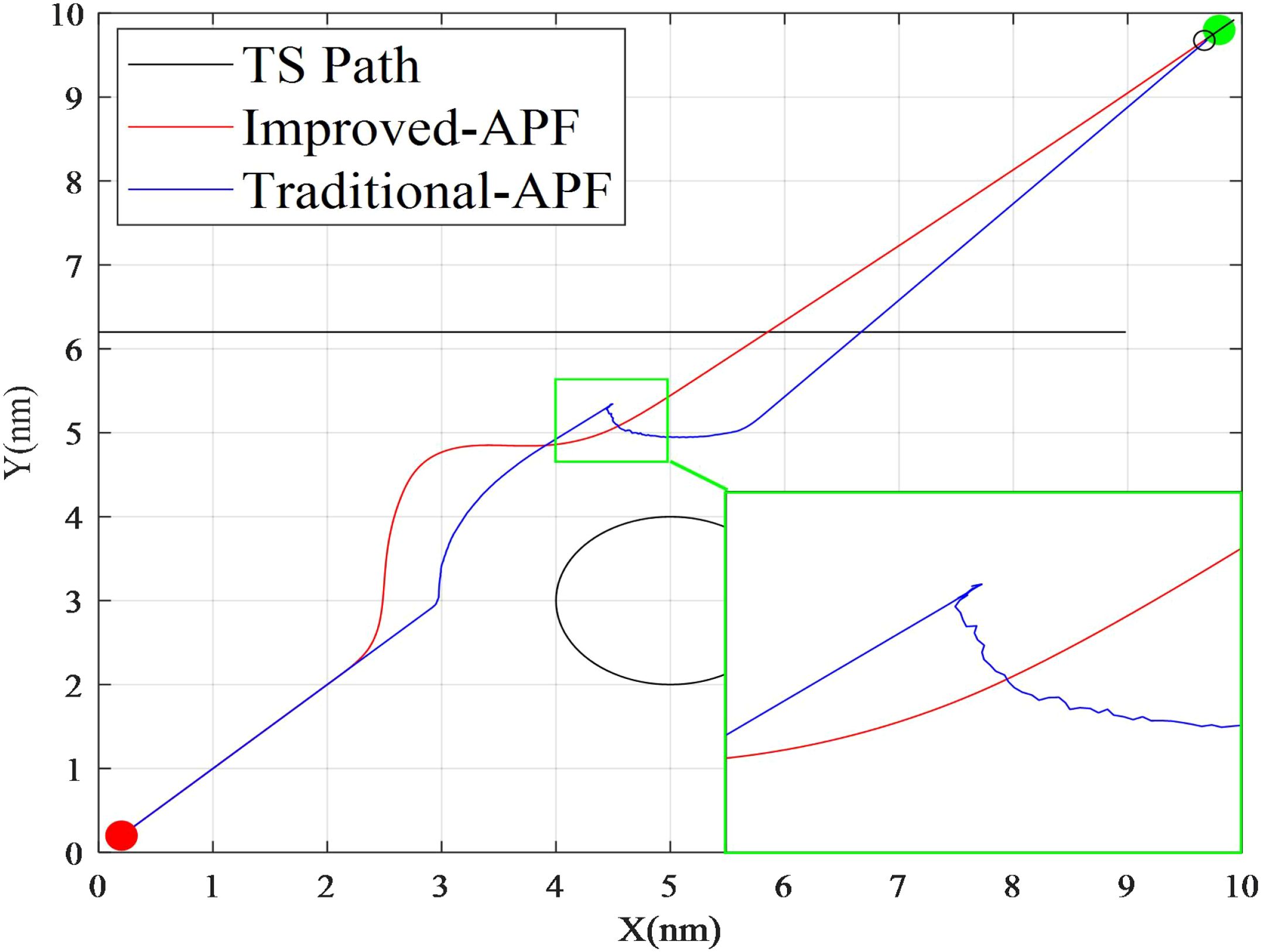
Figure 17. Comparison of simulation paths for Crossing1.

Figure 18 shows the speed and course change of the OS and the distance between the OS and TS in Situation 4. While the OS’s heading changes (about 280 iterations), the speed also decreases, and after about 350 iterations, the OS is successfully past and clear, and the OS’s speed also gradually returns to the upper limit, as unlike the previous four simulations the OS’s speed in the Crossing1 situation reaches the maximum speed of 12 knots. The improved-APF optimizes the speed adjustment in tandem with the course changes. As the OS turns to the starboard, its speed is adjusted to ensure that the turning radius is maintained without jeopardizing the ship’s stability. This smoother speed profile ensures that the OS avoids a collision efficiently without veering off course or risking excessive speed. The minimum distance achieved during this avoidance was recorded at 1.36 nm, a safe distance according to maritime safety standards, confirming the algorithm’s capability in avoiding potential collisions.

Figure 18

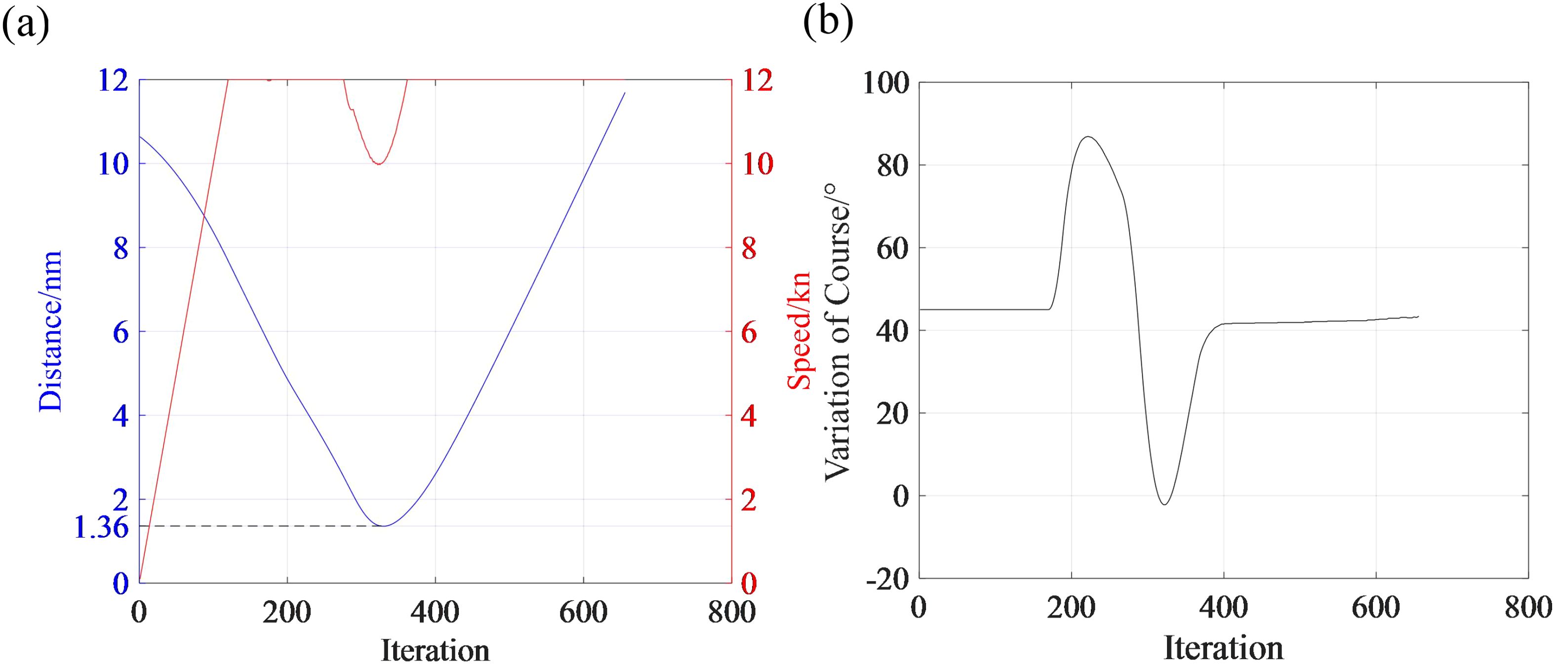
Figure 18. Situation 4 data change curve. (A) Distance between two ships and speed change of the OS. (B) Changes in the OS's course.

(5)Situation 5: Crossing2

The initial information of the OS for Crossing2 is position (10, 10), course (045°), and speed (0kn); while the initial information of the TS for Crossing2 is position (250, 500), course (180°), and speed (8kn).

In Situation 5 (Figure 19), according to the COLREGS for the crossing situation and quantitative analysis, the OS as the stand-on ship should have maintained its course and speed, but since this simulation set the give-way ship to navigate at a uniform speed, that is, “The vessel should keep her course and speed may however take action to avoid collision by her maneuver alone, as soon as it becomes apparent to her that the vessel required to keep out of the way is not taking appropriate action in compliance with these Rules”. As shown in the simulation, the traditional APF takes a longer route to avoid the TS, leading to excessive distance being covered, which reduces the efficiency of the maneuver. In real-world conditions, time is critical, especially in high-density traffic areas, and an overly long avoidance path could potentially lead to further collisions with other vessels. Moreover, the traditional APF still exhibits sharp angle turns, which result in path oscillations, further compounding the inefficiency and making the avoidance trajectory less predictable and harder to execute in practice. In contrast, the improved-APF algorithm delivers a significantly more efficient avoidance path, which is not only shorter but also smoother. This is largely due to the adaptive nature of the improved algorithm, which takes into account the ship’s current course and speed and the predicted future movement of the TS. The improved-APF anticipates the need for more gradual steering changes, which allows for precise and stable maneuvering while ensuring that the ship does not veer off course unnecessarily. The traditional APF does not make any effort to adjust the speed of the OS while performing the avoidance. This is problematic because, in practice, reducing speed during a maneuver helps maintain stability and control, especially when making sharp turns.

Figure 19

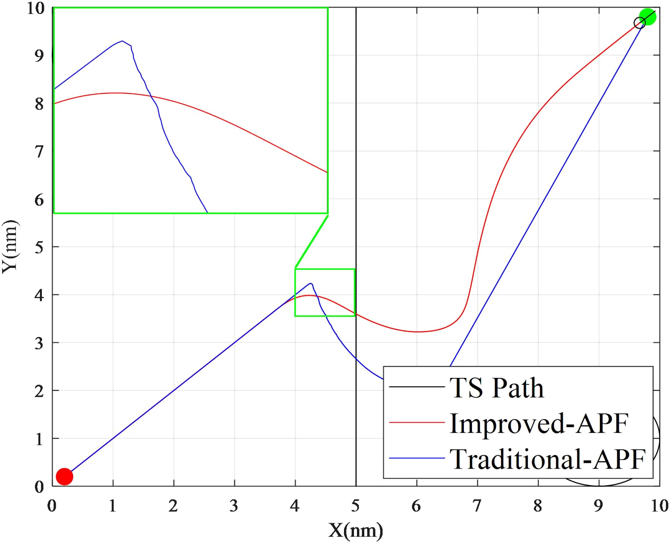
Figure 19. Comparison of simulation test paths for Crossing2.

Figure 20 shows the speed heading change process of the own ship and the distance change process between the own ship and other ships of the improved-APF in the cross-encounter situation 2. OS’s speed decreases while the own ship’s heading changes (about 280 iterations), and the TS is successfully past and cleared around 400 iterations, and the OS’s speed gradually returns to the upper limit and tries to return to course again in the subsequent navigation. The speed of the OS in Situation 5 reached 12 knots, and the distance curve between the two ships shows that the minimum distance during the avoidance process is 1nm, a safe distance according to maritime safety standards, confirming the algorithm’s capability in avoiding potential collisions.

Figure 20

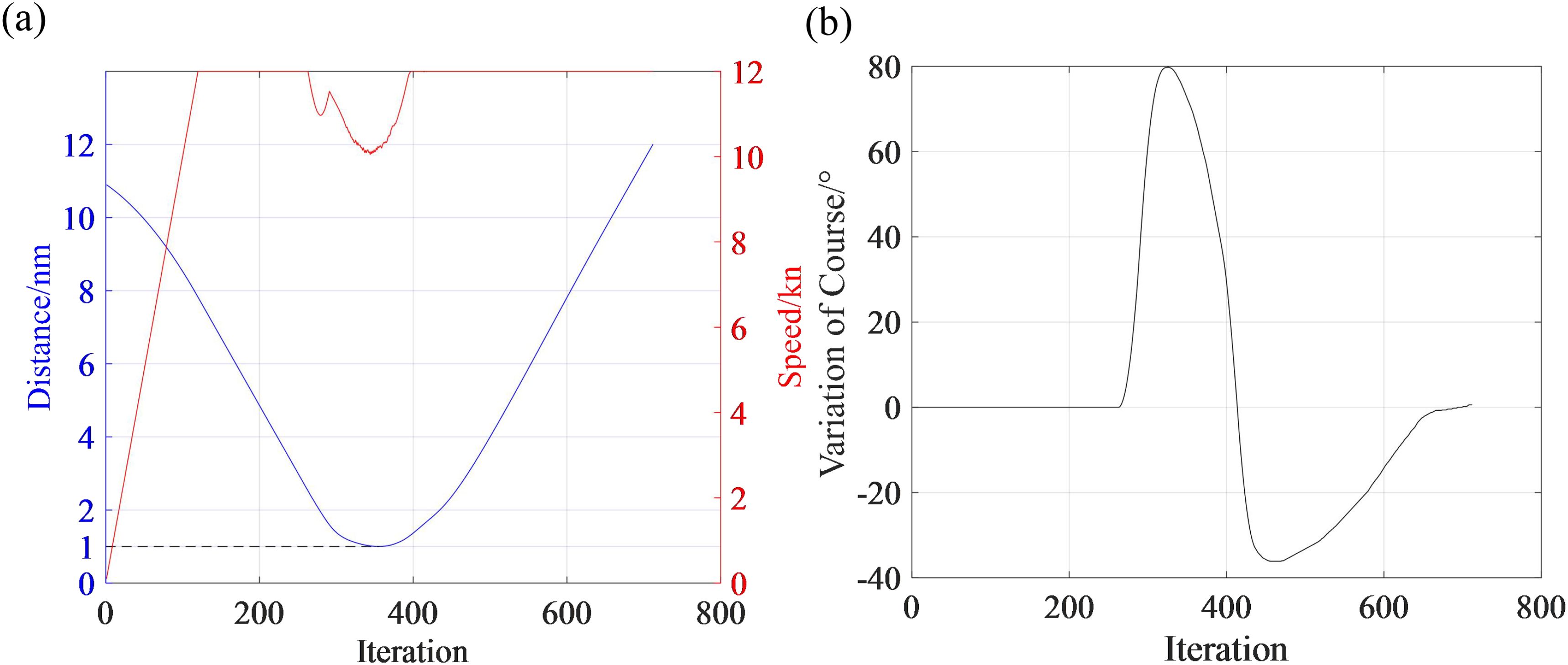
Figure 20. Situation 5 data change curve. (A) Distance between two ships and speed change of the OS. (B) Changes in the OS's course.

(6)Situation 6: Multi-situation

The initial information of OS for the Multi-situation is position (250, 10), course (000°), and speed (0kn); the initial information of TS1 for the Multi-situation is position (400, 200), course (243°), and speed (5kn); the initial information of TS2 for the Multi-situation is position (300, 350), course (180°), and speed (6kn); the initial information of TS3 for the Multi-situation is position (0, 350), course (090°), and speed (6kn); and the initial information of TS4 for the Multi-situation is position (200, 150), course(000°), and speed (2kn).

In Situation 6, Figure 21, the initial course of the OS crosses the course of TS1 and TS3, and it is give-way to TS1 and stand-on to TS3, and it is head-on with TS2 and in starboard overtaking with TS4. From Figures 21B, C, the OS steers starboard to cross the stern of TS1 and the bow of TS2 in 200 to 300 iterations, and steers port to cross the stern of TS3 in 500 to 600 iterations, and then turns starboard to avoid TS4 before heading straight to the target point.

Figure 21

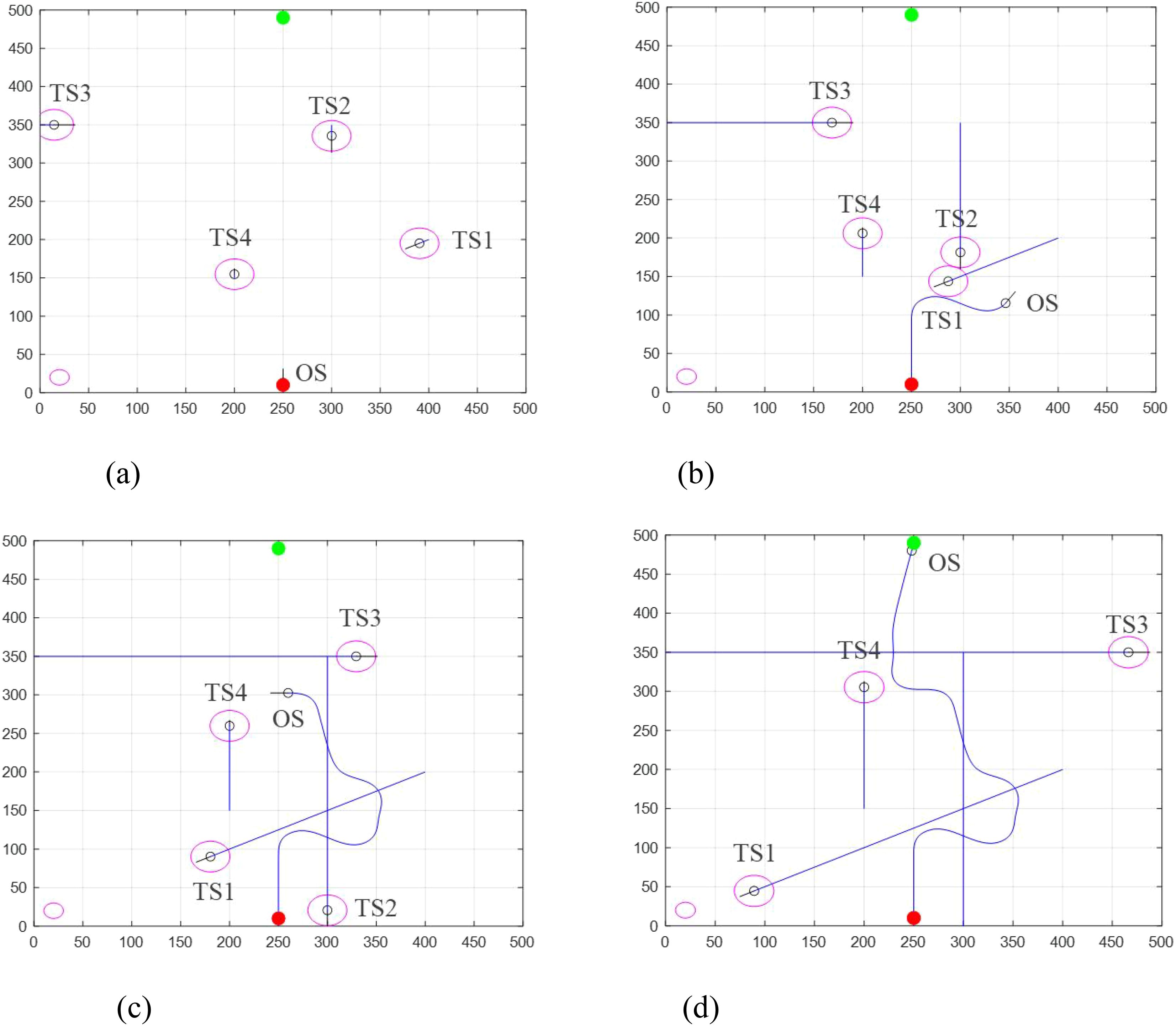
Figure 21. The collision avoidance process in a multi-situation. (A) Initial situation. (B) OS avoiding TS1 and TS2. (C) OS avoiding TS3 and TS4. (D) OS arrives at target point.

It can be seen in Figure 22 that the closest distances to TS1, TS2, TS3, and TS4 during OS avoidance are 0.84nm, 1.09nm, 1.24nm, and 1.09nm, respectively, safe distances according to maritime safety standards, confirming the algorithm’s capability in avoiding potential collisions.

Figure 22

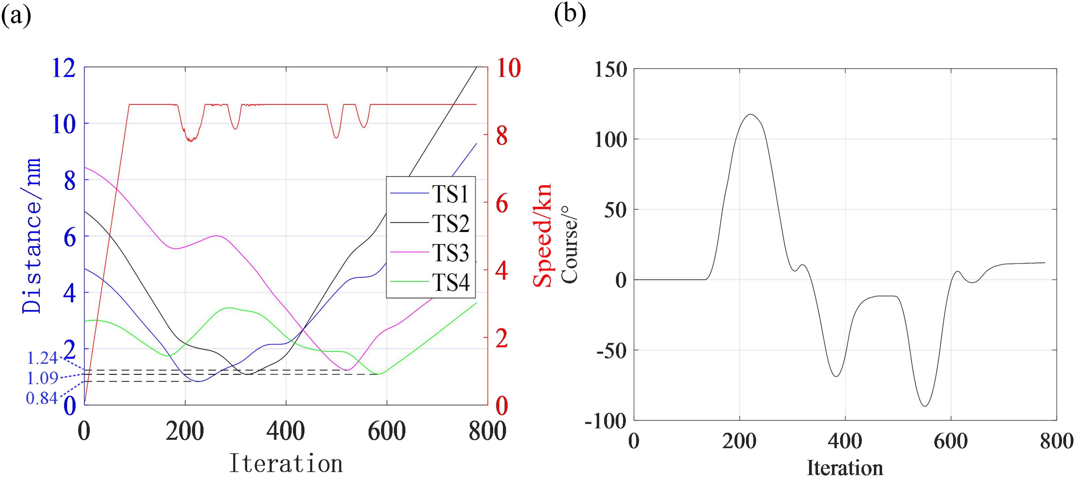
Figure 22. Situation 6 data change curve. (A) Distance between two ships and speed change of the OS. (B) Changes in the OS's course.

Considering the above experimental results, the improved-APF can complete a collision avoidance operation according to COLREGS requirements in the scenario of two-ship meeting in open water area, and the generated path is smooth and safe, which is in line with the reality.

From the distance curve between two ships, by introducing the quadratic ship domain to set the safety distance, the minimum distance between two vessels in six scenarios is kept above 0.4nm, which can ensure safe navigation.

It can also be seen from the speed change curve that the improved-APF does not simply steer during the avoidance operation but performs the deceleration operation at the same time to achieve maximum avoidance efficiency. After the collision avoidance operation, the algorithm also has the ability to resume the original heading after the avoidance operation is finished and the TSs are all past and clear.

In order to more accurately describe the smoothness of the path generated by the algorithm, this paper extracts the set of fitting points of each path, traverses the slope between each two points to obtain the slope set, and takes the absolute value of the difference between each adjacent two values in the set and sums them up, as a quantitative index to indicate the smoothness of the path. Thus, the closer to 0, the smoother the path is. The comparison results of the smoothness indexes by the improved-APF are 6.238 in head-on scenarios, 595.8 in overtaking scenarios, and 36.96 in crossing scenarios; while the comparison results of the smoothness indexes by the traditional APF are 92.14 in head-on scenarios, 1565 in overtaking scenarios, and 554.4 in crossing scenarios.

It can be seen that the improved-APF is better than the traditional APF in all the path smoothing degrees in compared simulation scenarios, and the overall smoothing degree was improved by 71.8%.

5 Conclusion

Ship collision avoidance decision-making methods have a wide range of applications in the field of unmanned or autonomous ships. In this field, factors such as collision avoidance in complex water areas and encounter scenarios have high requirements for ship navigation and control. This paper analyzes and summarizes the effect of the traditional APF algorithm on local dynamic collision avoidance of unmanned ships from the point of view of the ship’s maneuverability and COLREGS, and proposes a new autonomous collision avoidance decision-making method for unmanned ships, the improved-APF, which is applicable to actual navigation.

This paper introduces the feasibility and basic principles of the traditional APF in unmanned ship navigation and describes the problems associated with traditional APF such as path interference, path oscillation, and an unreachable target. The improved-APF proposed is introduced purposefully and its specific strategies are elaborated: the improvement of attractive-repulsive function and proposing of an own ship position posture selection mechanism based on the DWA and the requirements of COLREGS to make the generated trajectory smoother and more operable. Finally, the improved-APF is compared and analyzed using the MATLAB platform with static and dynamic obstacles to further verify the effectiveness and avoidance performance of the improved-APF. Furthermore, the experimental setup incorporates simulated environmental factors, such as composite potential fields formed by wind, waves, and currents, which adds complexity and realism to the collision avoidance simulations. The effectiveness and superiority of the algorithm were verified by comparing it with the traditional APF algorithm. The overall smoothing degree was improved by 71.8% and the effectiveness and superiority of the algorithm were verified.

However, there is still a gap between the simulation tests in this paper and the real scenarios. In further research, the improved-APF needs to be explored under the real-time influence of environmental factors, instead of updating every 100 iterations. A potential field model of the surrounding environment should be acquired and modeled in real time and integrated into the collision avoidance process. Additionally, the scalability of the algorithm could be explored, with the potential to extend its application to larger, more complex vessel fleets in congested waterways. Furthermore, studies could explore the combination of machine learning and reinforcement learning techniques with the proposed method to continuously improve the algorithm’s decision-making capabilities based on accumulated experience, making it more robust and efficient in varied maritime environments.

Data availability statement

The original contributions presented in the study are included in the article/supplementary material. Further inquiries can be directed to the corresponding author.

Author contributions

LL: Conceptualization, Data curation, Formal analysis, Funding acquisition, Investigation, Methodology, Project administration, Resources, Software, Supervision, Validation, Visualization, Writing – review & editing, Writing – original draft. WW: Conceptualization, Data curation, Formal analysis, Funding acquisition, Investigation, Methodology, Project administration, Resources, Software, Supervision, Validation, Visualization, Writing – original draft, Writing – review & editing. ZL: Conceptualization, Data curation, Formal analysis, Writing – review & editing. FW: Investigation, Methodology, Project administration, Writing – review & editing.

Funding

The author(s) declare financial support was received for the research, authorship, and/or publication of this article. This research was funded by the Central Guidance on Local Science and Technology Development Fund of Liaoning Province (No. 2023JH6/100100055), the Teacher Development Project of Dalian Maritime University (No. JY2022Y02), 2023 DMU Navigation College First-Class Interdisciplinary Research Project, (No.2023JXA01), and the Research Project on Education and Teaching Reform of the Navigation Technology Teaching Guidance Sub-committee of the Teaching Guidance Committee of the Ministry of Education for Transportation Majors in Colleges and Universities in China (No. 2022jzw004).

Conflict of interest

The authors declare that the research was conducted in the absence of any commercial or financial relationships that could be construed as a potential conflict of interest.

Generative AI statement

The author(s) declare that no Generative AI was used in the creation of this manuscript.

Publisher’s note

All claims expressed in this article are solely those of the authors and do not necessarily represent those of their affiliated organizations, or those of the publisher, the editors and the reviewers. Any product that may be evaluated in this article, or claim that may be made by its manufacturer, is not guaranteed or endorsed by the publisher.

References

Arimura K., Yamada S., Sugasawa Y., Okano (1994). Development of collisions preventing support system - model of evaluation indices for navigation. J. Japan Institute Navig. 91, 195–201. doi: 10.9749/JIN.91.195

Crossref Full Text | Google Scholar

Fiorini P. (1998). Motion planning in dynamic environments using velocity obstacles. Int. J. Robot. Res. 17, 760–772. doi: 10.1177/027836499801700706

Crossref Full Text | Google Scholar

Fiskin R., Atik O., Kisi H., Nasibov E., Johansen T. (2021). Fuzzy domain and meta-heuristic algorithm-based collision avoidance control for ships: Experimental validation in virtual and real environment. Ocean Eng. 220, 108502. doi: 10.1016/j.oceaneng.2020.108502

Crossref Full Text | Google Scholar

Gil M., Montewka J., Krata P., Hinz T., Hirdaris S. (2020). Determination of the dynamic critical maneuvering area in an encounter between two vessels: Operation with negligible environmental disruption. Ocean Eng. 213, 107709. doi: 10.1016/j.oceaneng.2020.107709

Crossref Full Text | Google Scholar

Howard R. A. (1960). Dynamic Programming and Markov Processes (New York: Technology Press-Wiley), 667.

Google Scholar

Iijima Y., Hagiwara H. (1991). Results of collision avoidance maneuver experiments using a knowledge-based autonomous piloting system. J. Navig. 44 (2), 194–204. doi: 10.1017/S0373463300009930

Crossref Full Text | Google Scholar

Khabit O. (1986). Real-time obstacle avoidance for manipulators and mobile robots. Int. J. Robot. Res. 5, 90–98. doi: 10.1177/027836498600500106

Crossref Full Text | Google Scholar

Kijima K., Furukawa Y. (2003). Automatic collision avoidance system using the concept of blocking area. IFAC Proceedings Volumes. 36 (21), 223–228.

Google Scholar

Kuffner J. J., Lavalle S. M. (2000). “RRT-Connect: An Efficient Approach to Single-Query Path Planning” in Proceedings 2000 ICRA. Millennium Conference. IEEE International Conference on Robotics and Automation. Symposia Proceedings (Cat. No.00CH37065), San Francisco, CA, USA, 2, 995–1001. doi: 10.1109/ROBOT.2000.844730

Crossref Full Text | Google Scholar

Lee M., Nieh C., Kuo H., Huang J. (2019). An automatic collision avoidance and route generating algorithm for ships based on field model. J. Mar. Sci. Technol. Taiwan 27, 101–113. doi: 10.6119/JMST.201904_27(2).0003

Crossref Full Text | Google Scholar

Lenart A. (1983). Collision threat parameters for a new radar display and plot technique. J. Navig. 36, 404–410. doi: 10.1017/S0373463300039758

Crossref Full Text | Google Scholar

Li L. Y., Wu D. F., Huang Y. Q., Yuan Z. M. (2021). A path planning strategy unified with a COLREGS collision avoidance function based on deep reinforcement learning and artificial potential field. Appl. Ocean Res. 113, 102759. doi: 10.1016/j.apor.2021.102759

Crossref Full Text | Google Scholar

Ma Y., Hu M. Q., Yan X. P. (2018). Multi-objective path planning for unmanned surface vehicle with currents effects. ISA Trans. 75, 137–156. doi: 10.1016/j.isatra.2018.02.003

PubMed Abstract | Crossref Full Text | Google Scholar

Rongcai Z., Hongwei X., Kexin Y. (2023). Autonomous collision avoidance system in a multi-ship environment based on proximal policy optimization method. Ocean Eng. 272, 113779. doi: 10.1016/j.oceaneng.2023.113779

Crossref Full Text | Google Scholar

Rothmund S. V., Tengesdal T., Brekke E. F., Johansen T. A. (2022). Intention modeling and inference for autonomous collision avoidance at sea. Ocean Eng. 266, 113080. doi: 10.1016/j.oceaneng.2022.113080

Crossref Full Text | Google Scholar

Selvam P., Raja G., Rajagopal V., Dev K., Knorr S. (2021). “Collision-free path planning for UAVs using efficient artificial potential field algorithm,” in 2021 IEEE 93rd Vehicular Technology Conference (VTC2021-Spring), Helsinki, Finland, 1–5.

Google Scholar

Tang P., Zhang R., Liu D., Zou Q., Shi C. (2012). “Research on near-field obstacle avoidance for unmanned surface vehicle based on heading window,” in Proceedings of the 24th Chinese Control and Decision Conference (CCDC), Taiyuan, China, 1262–1267.

Google Scholar

Thomas M. H., Colin J. G., Alonzo K., Dave F. (2008). State space sampling of feasible motions for high-performance mobile robot navigation in complex environments. J. Field Robotics. 25, 325–345. doi: 10.1002/rob.20244

Crossref Full Text | Google Scholar

Wang C., Zhang X., Gao H., Bashir M., Li H., Yang Z. (2024a). COLERGs-constrained safe reinforcement learning for realising MASS’s risk-informed collision avoidance decision making. Knowledge-Based Syst. 300, 112205. doi: 10.1016/j.knosys.2024.112205

Crossref Full Text | Google Scholar

Wang C., Zhang X., Gao H., Bashir M., Li H., Yang Z. (2024b). Optimizing anti-collision strategy for MASS: A safe reinforcement learning approach to improve maritime traffic safety. Ocean Coast. Manag. 253, 107161. doi: 10.1016/j.ocecoaman.2024.107161

Crossref Full Text | Google Scholar

Woo J., Kim N. (2020). Collision avoidance for an unmanned surface vehicle using deep reinforcement learning. Ocean Eng. 199, 107001. doi: 10.1016/j.oceaneng.2020.107001

Crossref Full Text | Google Scholar

Xu X. L., Zhou X. L., Cai P., Chu Z. Z. (2021). COLREGS-compliant dynamic collision avoidance algorithm based on deep deterministic policy gradient. Indian J. Geo Marine Sci. 50, 978–987. doi: 10.56042/ijms.v50i11.66794

Crossref Full Text | Google Scholar

Yang B., Li J., Ma J., Song W. (2017). Ship manoeuvrability parameter predictions of Yupeng. J. Jiangsu Univ. Sci. Technol. (Natural Sci. Edition) 31, 697–700. doi: 10.3969/j.issn.1673-4807.2017.06.001

Crossref Full Text | Google Scholar

Yu J., Liu Z., Zhang X. (2022). DCA-based collision avoidance path planning for marine vehicles in presence of the multi-ship encounter situation. J. Mar. Sci. Eng. 10, 529. doi: 10.3390/jmse10040529

Crossref Full Text | Google Scholar

Yuan X., Zhang D., Zhang J., Zhang M., Guedes S. C. (2021). A novel real-time collision risk awareness method based on velocity obstacle considering uncertainties in ship dynamics. Ocean Eng. 220, 108436. doi: 10.1016/j.oceaneng.2020.108436

Crossref Full Text | Google Scholar

Zaccone R. (2021). COLREGS-compliant optimal path planning for real-time guidance and control of autonomous ships. J. Mar. Sci. Eng. 9, 405. doi: 10.3390/jmse9040405

Crossref Full Text | Google Scholar

Zhang W., Deng Y., Du L., Liu Q., Lu L., Chen F. (2022). A method of performing real-time ship conflict probability ranking in open waters based on AIS data. Ocean Eng. 255, 111480. doi: 10.1016/j.oceaneng.2022.111480

Crossref Full Text | Google Scholar

Zhang K., Huang L., He Y., Wang B., Chen J., Tian Y., et al. (2023). A real-time multi-ship collision avoidance decision-making system for autonomous ships considering ship motion uncertainty. Ocean Eng. 278, 114205. doi: 10.1016/j.oceaneng.2023.114205

Crossref Full Text | Google Scholar

Zhang K., Huang L., He Y., Zhang L., Huang W., Xie C., et al. (2022). Collision avoidance method for autonomous ships based on modified velocity obstacle and collision risk index. J. Adv. Transp. 2022, 1–22. doi: 10.1155/2022/9604362

Crossref Full Text | Google Scholar

Zhang X., Wang C., Chui K. T., Liu R. W. (2021). A real-time collision avoidance framework of MASS based on B-spline and optimal decoupling control. Sens. (Basel) 21, 4911. doi: 10.3390/s21144911

PubMed Abstract | Crossref Full Text | Google Scholar

Zhang J., Zhang H., Liu J., Wu D., Soares C. G. (2022). A two-stage path planning algorithm based on rapid-exploring random tree for ships navigating in multi-obstacle water areas considering COLREGs. J. Mar. Sci. Eng. 10, 1441. doi: 10.3390/jmse10101441

Crossref Full Text | Google Scholar