Response of cetaceans to fluctuations of pelagic fish stocks and environmental conditions within the Celtic Sea ecosystem

Inshore waters off the south coast of Ireland are an important foraging area for a range of cetacean species. Some of the main prey species of these cetaceans are herring and sprat, two economically valuable fish species in the region. The Celtic Sea herring stock suffered a marked decline in 2013. The present study aimed to investigate potential changes in the ecosystem associated to the herring decline and to determine the potential impacts on predators. Here we analyzed sightings information of common dolphins, fin, minke, humpback and unidentified whale species, acoustic data of herring and sprat, and a range of environmental variables mainly derived from satellites. Firstly, we characterized spatio-temporal patterns in the relative abundance of predator and prey species, and environmental variables, and compared periods before and since the herring decline. Since the 2013 herring decline, (i) the herring stock has mainly concentrated in south-eastern coastal waters and southern offshore Irish waters, (ii) sprat density has increased, (iii) chlorophyll concentration has decreased, (iv) sea surface temperature has risen, and (v) the euphotic layer has extended deeper. Secondly, we modelled the effects of prey density and environmental conditions on the relative abundance and distribution of cetaceans, as well as the effects of environmental conditions on prey density, between 2005-2018 by applying Hurdle Generalized Additive Models. The models for herring and sprat support the idea that these species have different environmental relationships, for example herring tended to be found in shallower waters than was the case for sprat. The presence and relative abundance of common dolphins were significantly affected by both environmental conditions and herring density, whereas whale species presence and relative abundance were found to be correlated with sea surface temperature and prey density. The model results suggest differences in prey choice among whale species. Understanding the dynamic relationships between predators, prey and the environment is important to inform an ecosystem-based approach to fisheries management.

1 Introduction

The distribution and local abundance of cetaceans around the North Atlantic has been shown to be influenced by a range of environmental variables such as sea surface temperature, chlorophyll concentration, depth, wind components and large scale environmental indices such as the North Atlantic Oscillation index (e.g. Ramp et al., 2015; Tobeña et al., 2016; Prieto et al., 2017; Saavedra et al., 2017; Correia et al., 2019; Castro et al., 2020). Prey availability is also an important predictor (e.g. Pendleton et al., 2012; Zerbini et al., 2016). Cetaceans are often considered as opportunistic predators, modifying their diet in response to changes in prey availability (e.g. Piatt et al., 1989; Santos et al., 2013; Surma et al., 2018). To a large extent, the apparent influence of environmental predictors on cetacean distribution could be considered as a proxy for prey availability, although other factors such as thermal limits and diving capabilities are also relevant (e.g. Macleod et al., 2004; Lambert et al., 2014).

The Celtic Sea hosts a wide range and high abundance of cetacean species (O’Brien et al., 2009; Wall et al., 2013; Whooley and Berrow, 2019). Off the south and south-west coasts of Ireland, they are especially abundant during autumn and winter, when small pelagic fish concentrate in schools before migrating to spawning grounds (Molloy, 2006; Wall et al., 2013). Common dolphins (Delphinus delphis), fin (Balaenoptera physalus), minke (Balaenoptera acutorostrata) and humpback (Megaptera novaeangliae) whales are frequently recorded in this important foraging area (Whooley et al., 2011; Ryan et al., 2015; Volkenandt et al., 2015).

Common dolphins are piscivorous predators feeding mainly, on small pelagic shoaling fish, with preference for energy-rich species with high calorific content such as herring (Clupea harengus) and sprat (Sprattus sprattus) (Pusineri et al., 2007; Meynier et al., 2008; Spitz et al., 2010; Santos et al., 2014). Meynier et al. (2008) observed seasonal variation in the diet of common dolphins (i.e. species composition and prey size) which appears to be related to the availability of the prey species (e.g. sprat almost absent in the diet during winter and autumn). Similarly, Santos et al. (2013) demostrated that the observed lack of evidence for selective predation of common dolphins on sardine (Sardina pilchardus) may be related to the low stock abundance in the area. Dietary differences between inshore and offshore common dolphins in the Celtic Sea have also been observed. Specifically, in inshore individuals, herring and sprat account for the 1.2% and 2.3% of the total number of prey items respectively, while they were no present in the analyzed offshore common dolphins (Brophy et al., 2009).

In the study area, fin and humpback whales have been seen in association with seasonal inshore presence of spawning herring and sprat (Whooley et al., 2011; Ryan et al., 2013a; Volkenandt et al., 2015). Individual fin and humpback whales have shown some fidelity to the area. Fin whales have been recorded in five out of seven years surveyed by Whooley et al., 2011, while fidelity of humpback whales has been hypothesized from the high recapture frequency observed from a photo-identification study of 15 years developed by Ryan et al., 2015. Herring and sprat, especially age 0 (young of the year) fish have been identified as the main prey for baleen whales in the Celtic sea, together with northern krill (Meganyctiphanes norvegica) (Trenkel et al., 2005; Ryan et al., 2013a; Volkenandt et al., 2015; Baines et al., 2017). The proportion of these pelagic fish species in the diet of baleen whales in this area is high in comparison to other sites in the Northeast Atlantic and in the Mediterranean, where krill (mainly M. norvegica) is the major component of their diet (Gannier, 2002; Pierce et al., 2004; Visser et al., 2011; Ryan et al., 2013b; Víkingsson et al., 2014; Spitz et al., 2018).

Herring and sprat are key components of the ecosystem, transferring high-calorific energy to higher trophic levels (Pikitch et al., 2004; Engelhard et al., 2014). They are also valuable species for European and, specifically, Irish pelagic fisheries (Gerritsen and Lordan, 2014). The Celtic Sea ecoregion is one of the most productive pelagic fishing grounds in European waters (CSHMAC, 2018; STECF, 2019). Atlantic herring and sprat are the most important species (by weight) landed in European Union (EU) Member States in the Northeast Atlantic, accounting for 21.3% and 14.8% of the total catch respectively (Eurostat, 2020). Herring is also one of the most economically valuable commercial fish species in Ireland (Molloy, 2006; Marine Institute, 2013; O’Donnell et al., 2018). Irish boats take the majority of allocated total allowable catch (TAC) for herring inside the Exclusive Economic Zone (87% in 2012; Gerritsen and Lordan, 2014). Catches of both herring and sprat are mainly concentrated in the southern Irish waters (Gerritsen and Lordan, 2014).

Currently the Celtic Seas sprat stock is in assessment category 5, i.e. the only reliable source of information available to be used in an assessment is the landing declarations (ICES, 2017). According to published information, no clear trend has been detected in the abundance of the sprat stock over the study period. The status of the Celtic Seas herring stock is clearer. The raw acoustic abundance index obtained during the annual Celtic Sea Herring Acoustic Surveys (CSHAS) suggested a sharp decline since 2013 (O’Donnell et al., 2020), which was later confirmed by the stock assessment modelling initiated in 2012 (ICES, 2021b). Recruitment fell from 2011 to 2018 and since 2013 it has been below the long-term average. Even though an increase in the abundance of immature fish was observed in 2019 (O’Donnell et al., al., 2020), the perception of the status of the stock did not improve and the spawning stock biomass (SSB) remained under the Maximum Sustainable Yield approach (MSY B_trigger) since 2015 (ICES, 2021b). Fishing mortality (F) has been above the F_MSY level since 2015, although below the F_MSY level in 2020 (ICES, 2021a). It was concluded that the stock was being harvested unsustainably as a result of continued poor recruitment within the stock and ICES advised zero catches in 2020 and 2021 (ICES, 2019; ICES, 2020a; ICES, 2021a). In 2018, the Celtic Sea Herring Fishery lost its Marine Stewardship Council (MSC) certification (CSHMAC, 2018). In 2019, the main fishery closed early in the of the majority of sampled herring were below the Minimum Conservation Reference Size (ICES, 2020b).

At a smaller scale, the proportion of spawning herring in the autumn-western spawning ground of the Celtic Seas herring stock has declined since the 1990s (Harma et al., 2012; Volkenandt et al., 2014), dropping sharply in 2013, when no spawning was detected but, it was recorded in the winter-eastern spawning ground off the southern Irish coast (ICES, 2018a). While high fishing mortality seems to have been part of the problem, the changes seen in herring stock status may also be, at least in part, environmentally driven. Environmental conditions affect all life-stages of pelagic fishes, including the spawning success (Winters and Wheeler, 1996; Rijnsdorp et al., 2009; Brunel and Dickey-collas, 2010). Winter spawning has been shown to be favored over autumn spawning in years with warmer sea surface temperatures (Haegele and Schweigert, 1985). In other clupeid species such as sardine, variation in recruitment success and in abundance has been linked to environmental variation (e.g. Santos et al., 2012).

The decline of the Celtic Sea herring stock has led to concern about possible effects on predators such as cetaceans. Whooley (2019) found an unexplained decline in fin whale sightings during 2008 to 2018 in Irish offshore waters which could be related to changes in prey abundance. All odontocete and mysticete species are protected under national (Wildlife Act (1976) and Amendments) and international (EU Habitats Directive; Council Directive 92/43/EEC, 1992) law and within the Marine Strategy Framework Directive (MSFD; Directive 2008/56/EC, 2008). Moreover, cetaceans are considered indicator species under Descriptor 1 of Biodiversity of the MSFD for the assessment of the ocean health, and their monitoring is required for every EU member state (Santos and Pierce, 2015; Palialexis et al., 2019).

Here we investigated how cetacean distribution and abundance has changed with changes in prey availability, specifically the decline in herring over the past decade, in particular to the apparent decline of the herring stock during the study period (2005-2018). Since changes in fish distribution and abundance maybe at least partially driven by environmental factors, and both environmental conditions and prey availability are expected to influence cetacean distribution and abundance, we also examine the relationships between environmental factors, prey availability and cetacean abundance in the Celtic Sea. To address this aim, we compared ecosystem characteristics before and since the apparent herring stock decline, and we modelled the effects of environmental characteristics on the fish and the cetaceans, as well as the effect of fish density on local abundance of cetaceans using Hurdle Generalized Additive Models.

2 Materials and methods

2.1 Study area

The study area, to the south of Ireland, falls within the Celtic Sea Ecoregion as defined by ICES and includes portions of ICES Divisions 7.a, 7.b, 7.f, 7.g and 7.j.2 covering 87.065 km² between 11°- 5.5°W and 50.25°- 52.8°N (Figure 1).

FIGURE 1

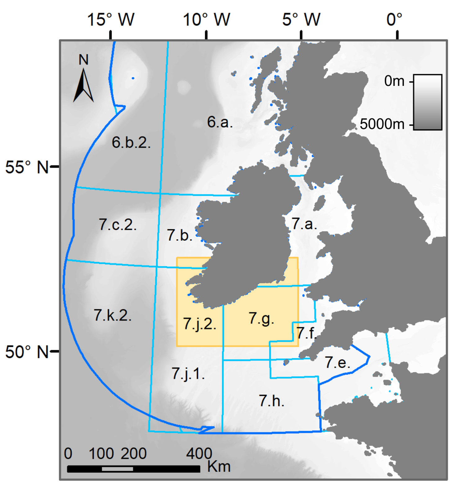
Figure 1 Map of the study area (yellow rectangle) and International Council for the Exploration of the Sea (ICES) Divisions (light blue lines) of the Celtic Sea ecoregion (darker blue line). The labels within the map indicate the names of the ICES Divisions, which shapefile was obtained from ICES website. The grey shading represents the bathymetry, which was obtained from General Bathymetric Chart of the Oceans (GEBCO) website.

The Celtic Sea is a shelf sea area strongly influenced by the North Atlantic Current, as well as by the Shelf Edge Current, the Irish Coastal Current and the Irish Shelf Front (Pingree, 1980). The water column in the shallower areas remains mixed over the whole year due to the action of the tides, while in deeper zones stratification occurs in summer, leading to lower productivity, which is interrupted by pelagic mesoscale structures such as productivity fronts (Pingree et al., 1982). Consistent with global warming, an increase in the average sea surface temperature of 0.3°C has been observed in Irish waters between 1850 and 2008, with the strongest warming trend detected in south-western waters (Cannaby and Hüsrevolu, 2009).

2.2 Data collection

Since 2004, the Marine Institute in Ireland has conducted an annual acoustic survey (Celtic Sea Herring Acoustic Survey - CSHAS) to derive an index of abundance of the Celtic herring stock, which is later used in the assessment models. The present study analyzed data collected during the surveys from 2005 to 2018. All CSHAS were conducted on-board RV Celtic Explorer and lasted for three weeks, typically between 6 and 26 October. Acoustic data were collected continuously (i.e. over 24 hours per day). Echo-integration was carried out for herring over the 24-hour period based on its behavioral characteristics in this region (no night time dispersion to surface waters) whereas echo-integration for sprat uses only data collected during daylight hours due its diurnal behavior and the effects of day-night bias (Cardinale et al., 2003).

Marine mammal and seabird (relative) abundance and distribution were determined through sighting surveys carried out during daylight hours. Data collection was interrupted only during trawl sampling and CTD deployments, since the vessel reduced speed (to 4 knots) or stopped, respectively. The vessel followed systematic parallel line transects and additional survey legs were carried out in areas of high herring abundance within the core survey area. The survey design and effort has changed only slightly between years, although the precise area covered has shifted over time to match shifts in fish distribution (O’Donnell et al., 2018; Figure 2A). The present study analyzed acoustic data on herring and sprat abundance, plus cetacean sightings, from 2005 to 2018.

FIGURE 2

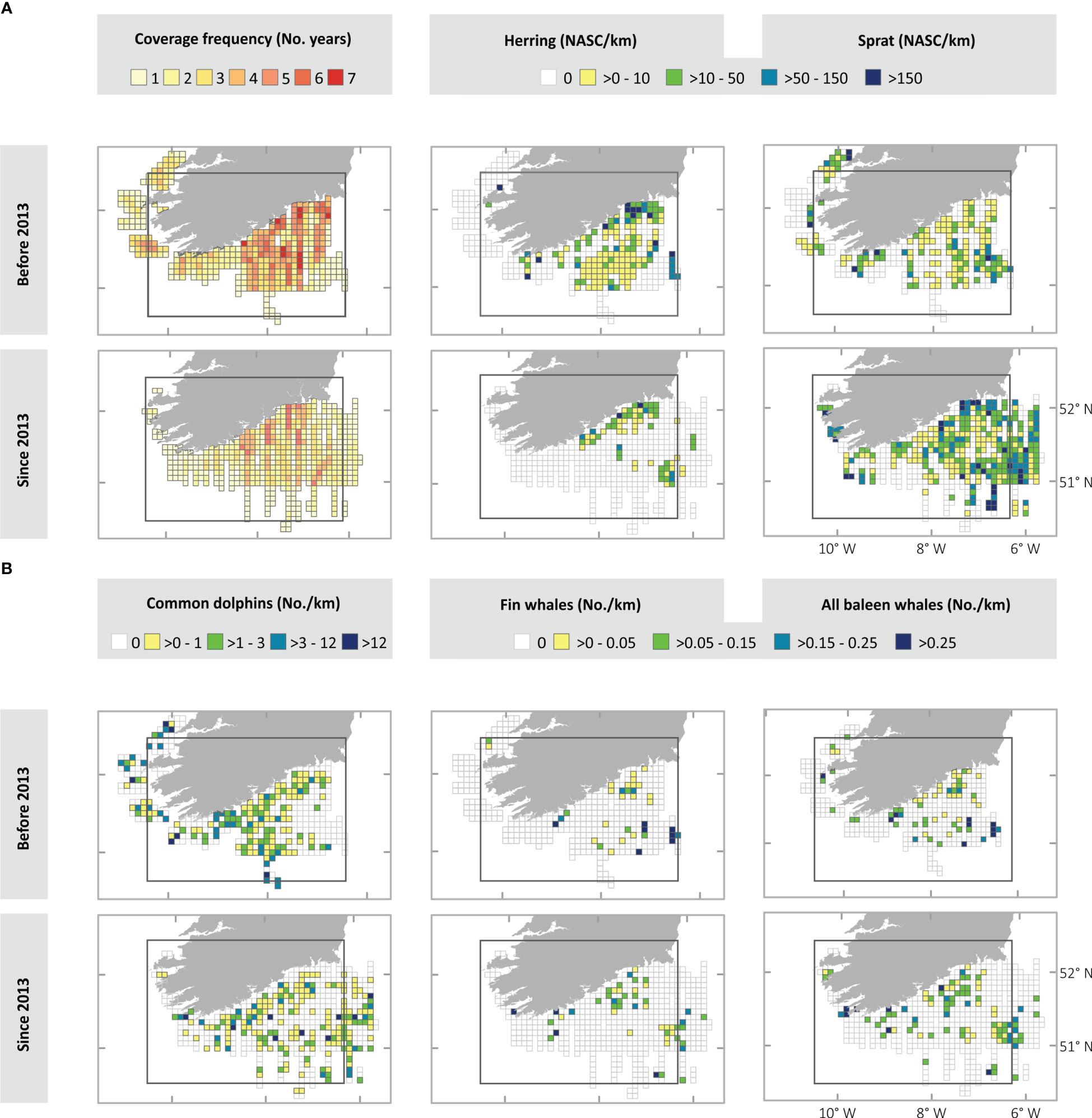
Figure 2 These maps represent spatialized data obtained from the annual Celtic Sea Herring Acoustic Surveys (CSHAS) in both study periods, i.e. before (from 2005 to 2012, 8 years) and since (from 2013 to 2018, 6 years) the herring decline. (A) First column of maps represents the area coverage by the surveys expressed as the number of years in which each cell grid was surveyed. Second and third columns of maps represent the relative abundance of the prey species before and since 2013. (B) Maps representing the relative abundance of the predator species before and since 2013. The grid cells (8 km x 8 km) represent the area sampled at least by one annual survey during each study period. The rectangle indicates the approximate area surveyed for all species and years of the study period, so apparent increases or decreases outside this area cannot be confirmed. NASC (Nautical Area Scattering Coefficient).

2.2.1 Environmental variables

We analyzed the relationships between the environmental conditions and the cetaceans response by using eight dynamic and two static environmental variables (Table 1), based on their known influence on cetacean distribution and abundance (Forney, 2000; Anderwald et al., 2012; Ramp et al., 2015; Tobeña et al., 2016), which is generally related to their expected influence on distribution of prey. The dynamic variables were the mean and standard deviation of: sea surface temperature (SST; °C), chlorophyll-a concentration (CHL; mg m^-3), photosynthetically available radiation (PAR; Einstein m^-2 day^-1), euphotic depth (ZEU; m), which were obtained from the Moderate Resolution Imaging Spectroradiometer (MODIS) on board the Aqua satellite (data available at the OceanColorWeb: https://oceancolor.gsfc.nasa.gov/l3/). Products of L3-SMI (Level 3 – Standard Mapped Images) with monthly and 4km resolution were downloaded and processed using Arc Macro Language in ArcGIS (ESRI, 2011) in order to transform distribution format to GIS-usable format. Data for the month when CSHASs are usually conducted and data from the previous and subsequent months (i.e. September, October, November) were used to calculate the average and standard deviation for each variable per grid cell per studied year (for further details about the number of records available for the analysis, see Table 1). Two static environmental variables, bathymetry and distance to coast, were also included. Bathymetry (with a 30-arc second resolution) was extracted from the General Bathymetric Chart of the Ocean (GEBCO: https://www.gebco.net/). Distances from the coast to the center of each grid cell were calculated in ArcGIS (ArcMap 10.4.1, ESRI, 2016) using the Near Table Proximity tool from the Analysis tool package (one value per grid cell).

TABLE 1

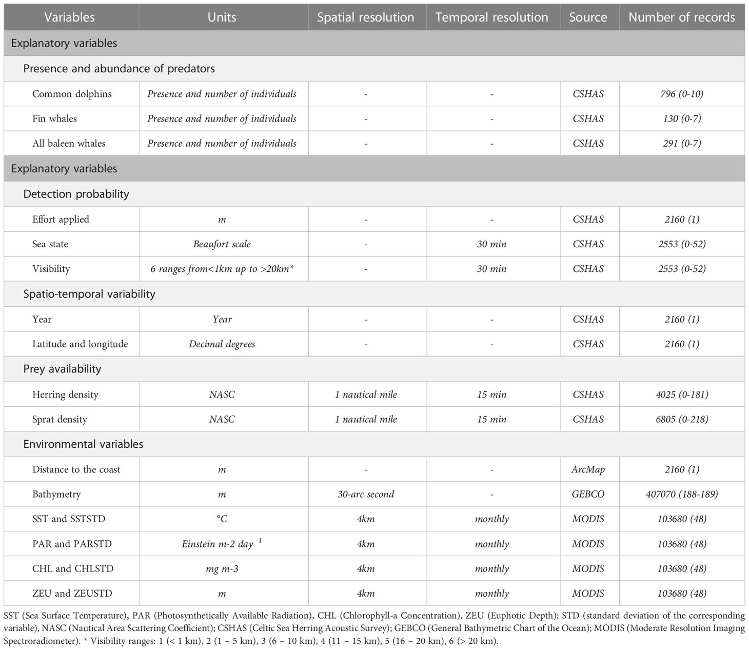
Table 1 Response and explanatory variables included in the models, units, spatial and temporal resolution, data source and total number of records followed by their range of values per grid cell per year between brackets.

2.2.2 Fisheries acoustic data

Acoustic information on the density of pelagic fish was collected using a Simrad EK60 scientific echosounder, operating with transducers at frequencies of 18, 38, 120 and 200 kHz. The nautical area scattering coefficient (NASC) was extracted and echo-integrated over the local sea depth for 1.85km horizontal segments into effort blocks known as elementary distance sampling units (EDSUs) (Simmonds and Maclennan, 2007). Echotraces were identified to species level and multi-species schools were catalogued as a mix of species, with the dominant species being specified when possible. Directed trawling was carried out to groundtruth the species composition of insonified echotraces. The process of when to trawl was largely subjective and carried out by a scientist with experience in school identification in this area.

Abundance and biomass estimates for the fish were available only at the scale of the whole study area, as annual snapshot estimates of abundance. Therefore, the raw acoustic (NASC) data were used for modelling the fine-scale prey-predator relationships. For a better understanding of the limitations of using NASC as a proxy of fish abundance, we explored the trends of the annual averages of (1) raw NASC values, (2) abundance and biomass estimated from the NASC (i.e. total stock abundance (TSN), spawning stock biomass (SSB; for herring) and total stock biomass (TSB; for sprat); O’Donnell et al. (2020)) and (3) recruitment calculated using the herring stock assessment models (ICES, 2021b). Following the Marine Institute’s protocols for the estimation of the abundance and biomass (O’Donnell et al., 2018), this study used only those echotraces identified as “definitely” or “probably” herring, sprat or a mixture of both in which one of these species was dominant. Thus, echotraces classified as “possible” herring or “possible” sprat (less than 2% of the total) were not included in the analysis.

2.2.3 Marine mammal data

Marine mammal observers (MMO) collected data on marine mammal sightings during daylight hours. Observations on effort were conducted in favorable weather conditions (sea state<6 and visibility >1km). Trained and experienced MMOs were used during each survey and in some cases two marine mammal observers were onboard. In such instances, observers alternated with each other to maximize observer effort during daylight hours. Observers scanned the horizon by eye, focusing 90° either side of the survey track line, and using binoculars when required (e.g. to confirm species identification and group size). The main observation platform was the crow’s nest, situated 18m above sea level, but if weather conditions were unsuitable, observations were conducted from the ships bridge, which was located at 11m above sea level. Logger 2000 software (IFAW, 2000) was used to store the sightings information and environmental conditions. The latter were recorded every 30 minutes or whenever conditions or the survey track line changed. Sightings data recorded included location, time, species, number of individuals, sea state (Beaufort scale) and visibility (on a six-point scale: 1 =< 1km, 2 = 1 – 5km, 3 = 6 – 10km, 4 = 11 – 15km, 5 = 16 – 20km, 6 =>20km). Whenever identification to species level was not possible, cetaceans were identified to the nearest possible taxonomic level (e.g. dolphin species or large whale species).

Data from three types of cetaceans were analyzed, including the two most frequently sighted species, namely common dolphins (n=410) and fin whales (n=83). In order to account for the other baleen whale species (which had a low number of observations when considered separately), fin, minke, humpback whales together with unidentified baleen whales were treated as a third category, i.e. “all baleen whales” (n=160). All sightings recorded on-effort were included in the present analysis, whether or not conditions were suitable for detection of cetaceans (Barlow, 2015). To account for the lower probability of seeing animals in poorer conditions (i.e. extrinsic variability of the response variable), sea state and visibility were included in the models as explanatory variables.

2.3 Data processing

Data were imported and processed in ArcGIS using tools available in ArcToolbox (ArcMap 10.4.1, ESRI, 2016). In order to avoid possible distortion of some spatial features from differing data sources a customized Projected Coordinate System, centered on the study area (i.e.: central meridian = -8.5°; latitude of origin = 51.5°; scale factor = 1), was created for the project (MacLeod, 2013).

A fixed square grid was created using the “Fishnet” tool and used in order to extract the final data in a standardized format. The cell size was set at 8 x 8 km based on knowledge of the effective prey detection range for baleen whales in the Celtic Sea - estimated at 8km by Volkenandt et al. (2015), the association distance between common dolphins with their prey - estimated as between 0 and 14.82 km in the Bay of Biscay by Lambert et al. (2018), and considering the spatial resolution of the oceanographic variables (4km).

Only segments of the tracklines for which the echosounder and MMO were simultaneously on effort were included. Using a combination of Intersect and Spatial Join tools, the cetacean sightings (numbers of individuals of each species, and presence/absence), together with the prey detections (average NASC values, and presence/absence) and oceanographic data (dynamic and static variables) were extracted per cell grid for each year. For creating the relative abundance maps of the prey and cetacean species, cetacean sightings and prey NASC data were standardized by dividing the total number of detections by the total length (km) of the segments on common effort in each grid cell (i.e. total number of individuals or sum of NASC values per km on effort by species). For modelling the data were not standardized by effort because effort was included as an explanatory variable in the models.

2.4 Data analysis

A detailed data exploration was carried out in R statistical software (R Core Team, 2018) following recommendations by Zuur et al. (2010) to assess possible outliers, normality, distribution, collinearity and relationships among the variables. After examining the distributions of the sightings and acoustic data and fitting some preliminary models, several outliers were detected all associated with grid cells with low survey effort. In order to exclude these outliers we excluded all grid cells with less than 500m of effort. Fifteen cells out of 2176 were thus removed, 5 of which had cetacean sightings and 10 of which had detections of sprat. In addition, herring and sprat NASC variables were log-transformed due to having right-skewed distributions, i.e. the majority of values were concentrated at the lower end of the range with very few high values. Potential outliers were identified based on hat-values (a hat-value of 1 or over indicates a data point with unacceptably high influence on the model results; see Zuur et al., 2007). Three cetacean detections were excluded from the analysis because of the unusually high number of individuals recorded in the cell (even if genuine) could unduly influence the model output. Collinearity among explanatory variables was assessed by Pearson correlation matrices and visualization in pair plots. Mean CHL was excluded from subsequent analysis since it was highly correlated with the its standard deviation (CHLSTD) and several other explanatory variables (Supplementary Figure 1). Due to its right-skewed distribution, CHLSTD was log-transformed to reduce the influence of very high values.

2.4.1 Spatio-temporal characterization

In order to provide an overview of the changes which have occurred in the distributions of the predator and prey species studied and the ecosystem conditions, we examined the trends over time and compared spatial distributions from 2005-2012 and from 2013-2018, i.e. before and since the herring decline (accordingly with the NASC values used in this study).

Prior to comparing the abundance indices for prey and predators and the oceanographic conditions, between the two periods, it is necessary to consider the annual survey coverage. Consequently, we represented the distribution and frequency of the effort applied in graduated color maps. These maps show the variation on effort over the study timeframe, adapting to the changes in herring distribution. Temporal trends in predator and prey species were observed and compared by time series graphs of the annual averaged abundance index values. Additionally, as mentioned in previous section 2.2.2. for herring and sprat we compared the annual averages of (1) raw NASC values, (2) abundance and biomass estimated from the NASC (i.e. TSN, SSB and TSB; O’Donnell et al., 2020) and (3) recruitment calculated using the herring stock assessment models (ICES, 2021b), to provide a better understanding of the relationships among these stock parameters. For the dynamic oceanographic variables, the temporal trends of their values and the changes over the studied period, were visually compared using a heatmap, an Integrative Trend Analysis technique (ICES, 2018b) which represents the individual variation of different types of variables, all normalized to range between 0 and 1, by graduated colors.

We produced maps for both periods using ArcGIS (ArcMap 10.4.1, ESRI, 2016). The averaged density (NASC) for the pelagic fishes and the average number of individuals for cetacean species, both variables standardized per unit of effort for each of the grid cells, were calculated to represent the relative abundance of both prey and predator species by graduated colors. For a better understanding, we produced a map representing the distribution of prey and predator species including all grid cells surveyed at least once during each study period (i.e. before and since the herring decline; Figures 2A, B) and another map representing all the squares covered (at least once) in the whole study period (Supplementary Figure 2).

2.4.2 Modelling

Regarding the oceanographic conditions, in order to support their characterization using visual tools as described below, models were also applied. General Additive Models (GAMs) were fitted with a gamma distribution family and log link function, to the time series of annual average values for every oceanographic variable and we also compared values before and since 2013 (Equations 1 and 2, using the variable CHL as an example):

$\begin{array}{ll}\text{gam }(CHL~s(Year),\text{ family}=\text{Gamma }(\text{link}=“\text{log}”))& \text{(Equation 1)}\end{array}$

$\begin{array}{ll}\text{gam }(CHL~Periods,\text{ family}=\text{Gamma }(\text{link}=“\text{log}”))& \text{(Equation 2)}\end{array}$

where Periods is a Bernoulli variable in which the years 2005-2012 take the value 0, and for years 2013-2018 take the value 1.

Concerning predator and prey occurrence and distribution, models were used to explore the relationships among ecosystem components. Exploration of the data suggested the existence of non-linear relationships between predator and prey response and explanatory variables; therefore, Generalized Additive Models (GAMs) were used. These models are one of the recommended techniques for developing an integrative trend analysis to explore the relationships among ecosystem components including different trophic levels and environmental variables (ICES, 2018b). Moreover, they are extensively used for cetacean habitat modelling and prey-predator interactions studies (e.g. Nøttestad et al., 2015; Zerbini et al., 2016; Derville et al., 2018; González García et al., 2018; Virgili et al., 2019).

Specifically, Hurdle GAM models (models in two stages) (Cragg, 1971) were used to deal with the large number of zero values in our cetacean and prey count data. For the first stage, a binomial distribution and logit link function were used to fit a model to presence-absence data on the cetaceans and fish. For the second stage, the presence only data were modelled, using a negative binomial model with logit link function and the optimizer ‘perf’ was used (the data did not fit well to a Poisson distribution, e.g. Supplementary Figure 3) for cetacean models, and a gamma model with log link function for fish abundance models. The theta value showed little variation between different models for a given taxonomic group and the theta value was therefore not fixed. Models were fitted using the ‘mgvc’ library (Wood, 2013) in the R software (R Core Team, 2018).

The cetacean models included six response variables: annual presence/absence (i.e. sighted animals or not) and relative abundance (i.e. number) of common dolphins, fin whales and all baleen whales in each grid cell per year. The explanatory variables fall into several categories: variables affecting the detection probability of cetaceans (observation effort, sea state and visibility conditions), spatio-temporal variables (year, latitude and longitude), prey availability (densities of herring and sprat), static environmental variables (depth and distance from the coast), and oceanographic variables (SST, CHL, PAR, ZEU and their standard deviations) (Table 1). Firstly, we explored the extrinsic variability of cetacean presence and abundance due to their detection probability using this category of variables. Then, three different sets of models were run with the spatio-temporal, prey and environmental variables. Lastly, models were fitted using explanatory variables from all the above subsets.

The prey models included four response variables: the presence/absence and acoustic density (i.e. NASC values) of herring and sprat. The explanatory variables used were the recorded variables that could affect to the echosounder (time on effort and sea state), as well as the static environmental and dynamic oceanographic variables used in the cetacean models. A general model for each prey response variable was constructed using all the mentioned explanatory variables.

To avoid over-fitting and ensure that biologically realistic relationships were obtained, the degrees of freedom for the smoothers for the explanatory variables were limited to a maximum value of 3 by setting the number of knots (k) at 4, following recommendations by Wood (2006) and agreeing with other studies (e.g. González García et al., 2018; Virgili et al., 2019). The spatiotemporal variables are expected to have more complicated effects on the response variables so higher numbers of knots were permitted for the variables Year and Latitude x Longitude (latitude and longitude were included in the same smoother term thus accounting for their main effects and their interaction). The function ‘gam.check’ was used to verify that the number of knots used was adequate.

Optimal models for both predator and prey species, were determined following a forward stepwise selection process based on the Akaike information criterion (AIC; Anderson and Burnham, 2002) as well as considering the significance of the explanatory variables (p-values), deviance explained and R². In general, the most suitable models were selected based on the lowest AIC. Where two models had similar AIC values (δAIC<2) an ANOVA Chi-square test was used to verify their similarity, and where similar models differed in complexity applied the principle of parsimony (i.e. giving preference to the simpler model). The final models assumptions were validated by checking for outliers or influential values and the homogeneity of variance (by fitted values vs residuals plots). When a hat value higher than 1 was identified (indicating a data point with high influence), the corresponding model was compared with and without that value. The performance of the model was validated by testing the correlation between fitted values (after inverse transformation) and observed values (Spearman test) and checking these results visually by plotting fitted values vs observed values. The results from the Spearman test are included in the Supplementary Table 4.

For the interpretation of the effects of the significant continuous exploratory variables included in the models, we looked at the partial effects plots from the GAMs output. When a horizontal line (i.e. zero trend) could be fitted within the 95% confidence intervals illustrated in these plots, the trend (within the relevant range of values of the explanatory variable) could be considered non-significant. This was frequently relevant for the extreme values of the explanatory variables, where the wide 95% confident intervals reflect the lower number of observations.

3 Results

3.1 Exploratory analysis of the spatio-temporal variation

3.1.1 Survey effort

A total of 16,718.8 km (a daily average of 59.7 km) was covered (simultaneously) by both MMOs and echosounder on effort during 280 days from 14 surveys. The frequency of coverage per cell grid showed differences between periods before and since 2013 (Figure 2A). The south-western coast of Ireland was surveyed only during the first period, while more effort was applied in the south-eastern part of the study area since 2013, because of the survey adapting to evidence of changes in the distribution of herring and commercial fishing effort (Ciaran O’Donnell, Personal observation, 5^th October 2021). The central zone accumulated most of the effort over the whole time series.

3.1.2 Oceanographic variables

Several trends in the oceanographic variables were observed from the models, maps and heatmap. CHL was lower since 2013 (Figure 3) decreasing significantly between 2009 and 2014 and increased in the last years (p<0.0001, Supplementary Figure 4; Supplementary Table 1), which is especially noticeable in coastal zones (Figure 4). CHLSTD has also decreased significantly in the latter period (p=0.001, Supplementary Figure 4, Supplementary Table 1 and Figure 3) showing a spatial pattern which reflects weaker variability in oceanic waters and stronger variability in coastal areas, although this trend was less clear since 2013 (Figure 3). In addition, euphotic depth (ZEU) has increased since the herring decline (Figures 3, 4) significantly from 2009 to 2014 (Supplementary Figure 4; Supplementary Table 1), specifically in central and southern areas, while its variability (ZEUSTD) was higher in coastal waters in both periods (Figure 4).

FIGURE 3

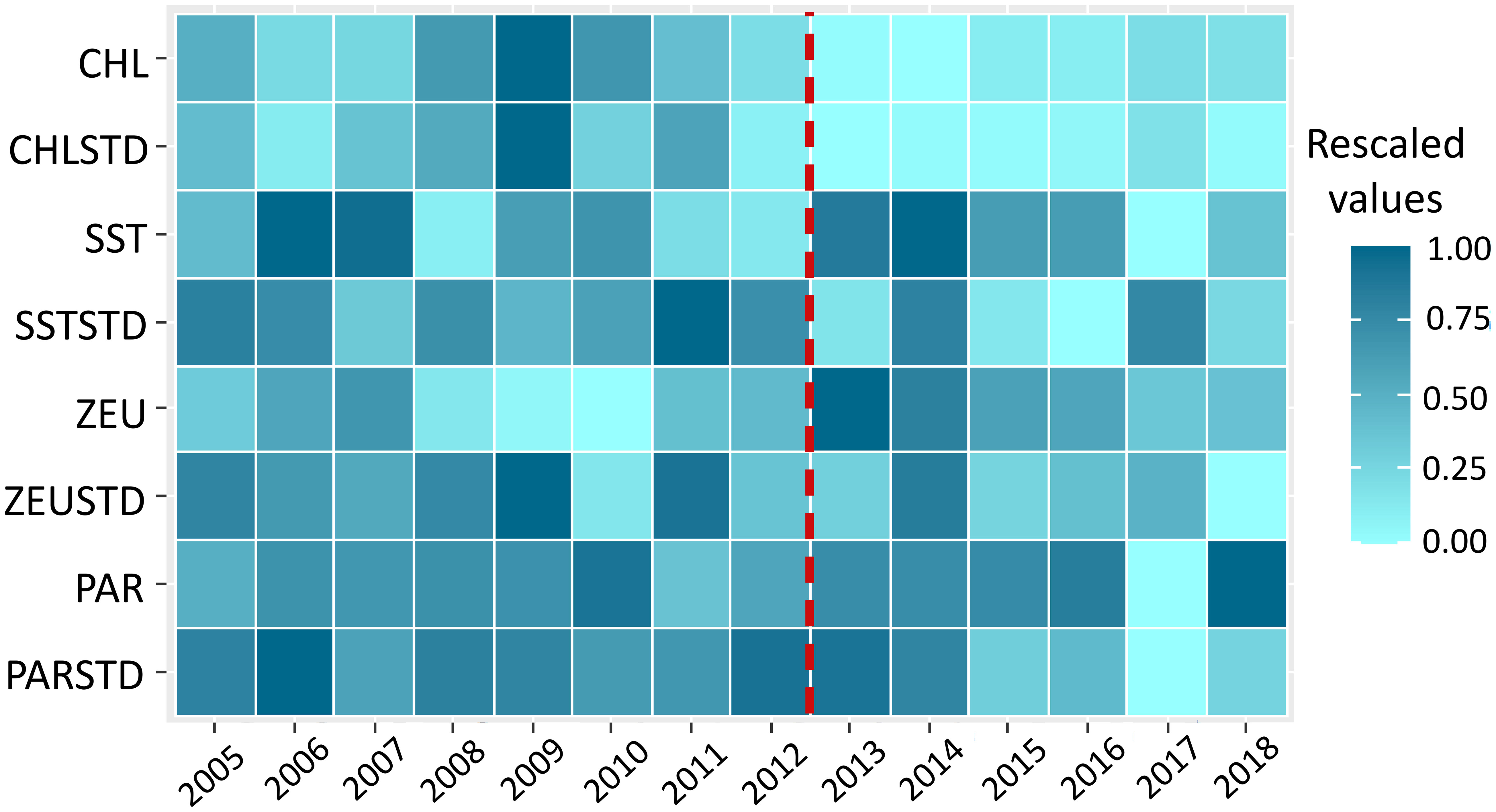
Figure 3 Heatmap representing the temporal trends of the oceanographic variables included in the study rescaled between the values 0 and 1. The lightest blue represents the minimum value of the annual average over the study area of each variable, while the darkest represents the maximum. The red dashed line highlights the year since the herring began to decline. Variables represented on Y-axis are: chlorophyll concentration (CHL); sea surface temperature (SST); Euphotic Depth (ZEU); Photosynthetically Available Radiation (PAR); and the standard deviation of the oceanographic variables (CHLSTD; SSTSTD; ZEUSTD; PARSTD). Data source: OceanColorWeb.

FIGURE 4

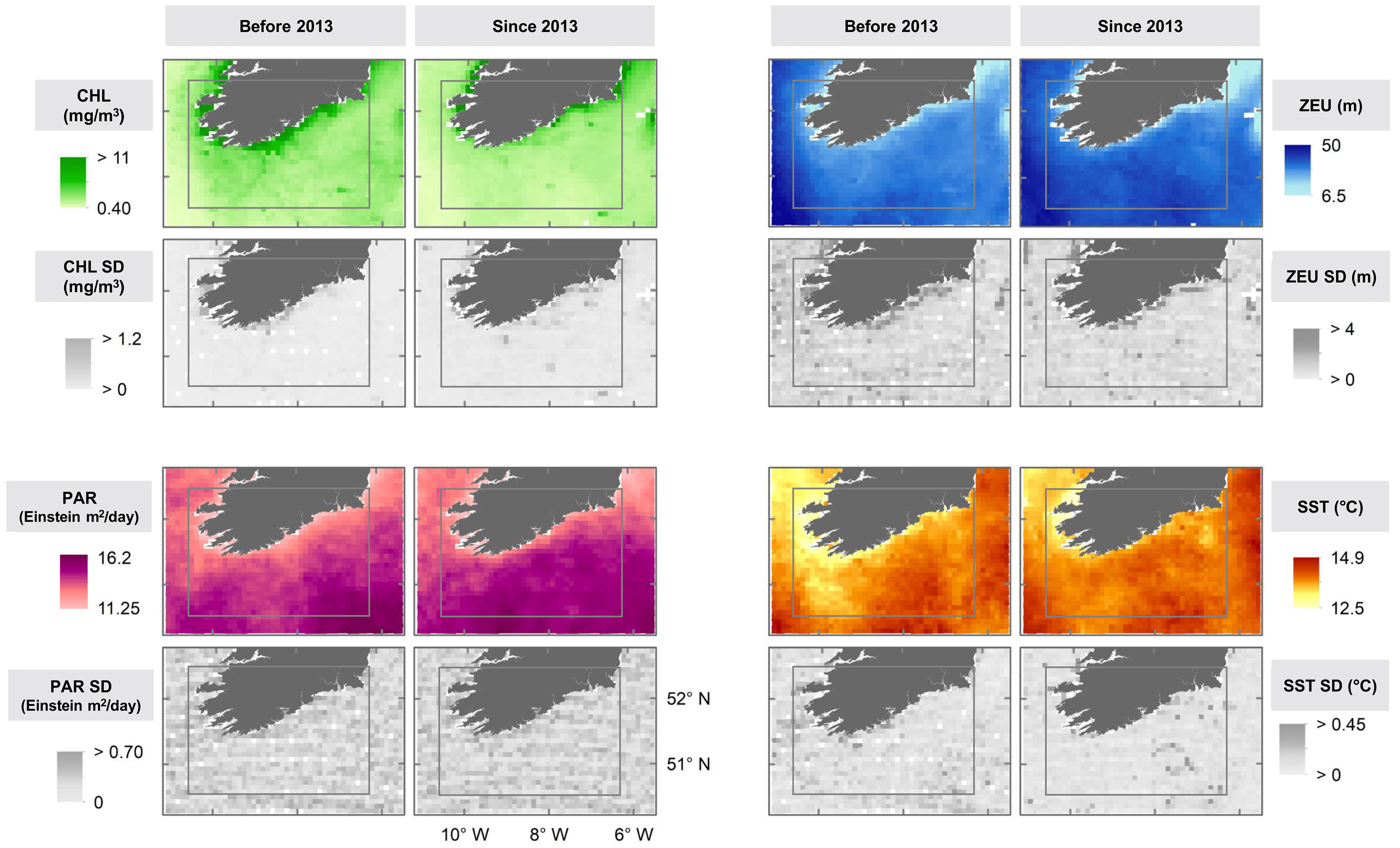
Figure 4 Maps showing the spatial patterns of the average annual mean and standard deviations (SD) between the periods 2005-2012 and 2013-2018 of the four oceanographic variables included in the study: Chlorophyll concentration (CHL), Euphotic Depth (ZEU), Photosynthetically Available Radiation (PAR) and Sea Surface Temperature (SST). The rectangle indicates the approximate area surveyed for all species and years of the study period. Data source: OceanColorWeb.

From the maps of another proxy of primary productivity (Photosynthetically Available Radiation, PAR) it appears to have increased considerably in recent years, more so in coastal and adjacent waters as well as in the strip between coordinates 10° W – 8° W (Figure 4). However, no significant trend was found from the GAMs results (Supplementary Table 1). From the heatmap, lower variability of PAR (i.e. lower PARSTD) in also apparent from the heatmap over the last few years of the study period (Figure 4) and from the significant results from the corresponding model (p=0.005, Supplementary Figure 4; Supplementary Table 1). The maps (Figure 4) show an increase of SST since the herring decline in both the south west and south east of the study area, although it is more noticeable in the former zone. In the same areas, the variability of sea surface temperature (SSTSTD) was stronger before 2013 and more evident in the south east since then. Despite some apparent contradictions in the signals, it appears that productivity was lower after the herring decline.

3.1.3 Prey and cetacean species occurrence and distribution

Over the study period, herring SSB and TSN followed very similar trends, differing from both NASC and recruitment. It appears that between 2008 and 2010, SSB and TSN increased while NASC remained stable near its lowest values. The average NASC showed three peaks, the largest occurring in 2012 and corresponding to peaks in SSB and TSN. Since then, these three parameters decreased sharply. Slightly earlier, the herring recruitment estimated by the stock assessment models, showed a peak in 2011 from which it decreased until the end of the study period (Figure 5).

FIGURE 5

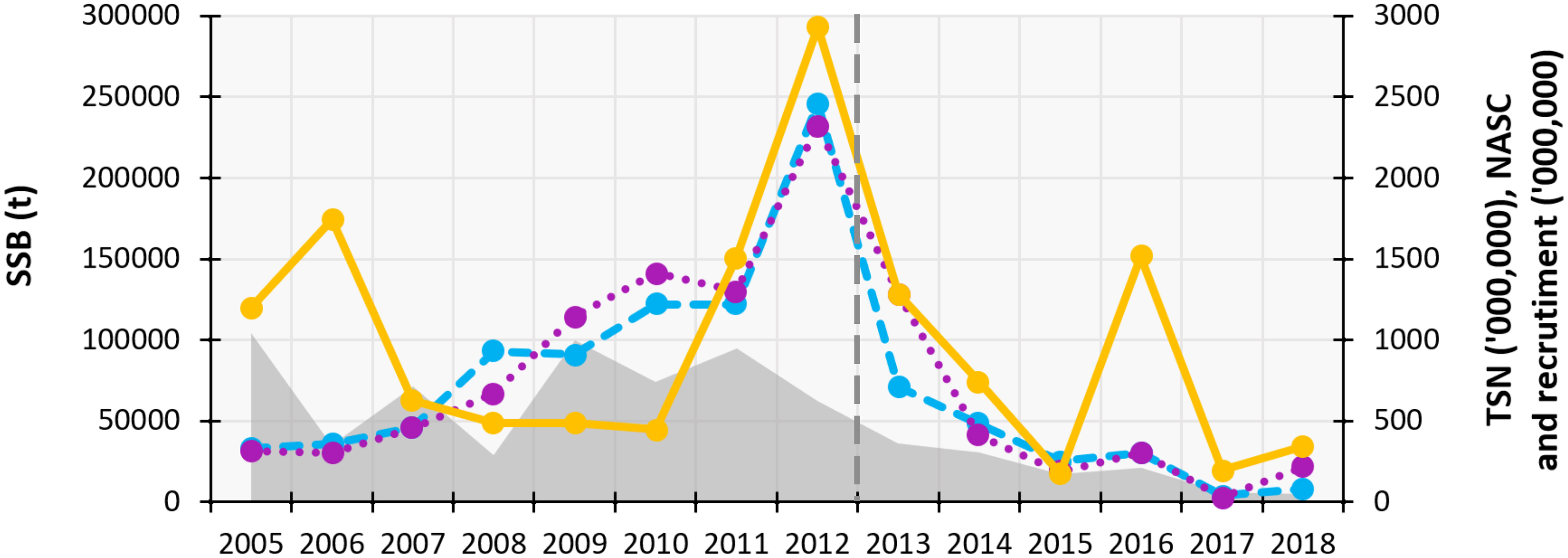
Figure 5 Time series graph representing the herring (Clupea harengus) annual average values of the Total Stock Abundance (TSN, millions of fish, right axis; purple dotted line), Spawning Stock Biomass (SSB, t, left axis; blue dashed line), Nautical Area Scattering Coefficient (NASC, unitless, right axis; orange solid line), recruitment (millions of fish, right axis; light grey shaded area) and year since the herring began to decline (dark grey dashed line). Data source: Annual Celtic Sea Herring Acoustic Surveys, except for the recruitment which was calculated from the herring stock assessment models by ICES (2021b).

The sprat stock indicators TSN and TSB showed similar trends, with an increase from 2007 to 2015 and a second peak in 2017 (higher than in 2015 for TSN but lower than 2015 in the case of TSB). The NASC trend was again different, reaching a maximum value in 2013 (Figure 6).

FIGURE 6

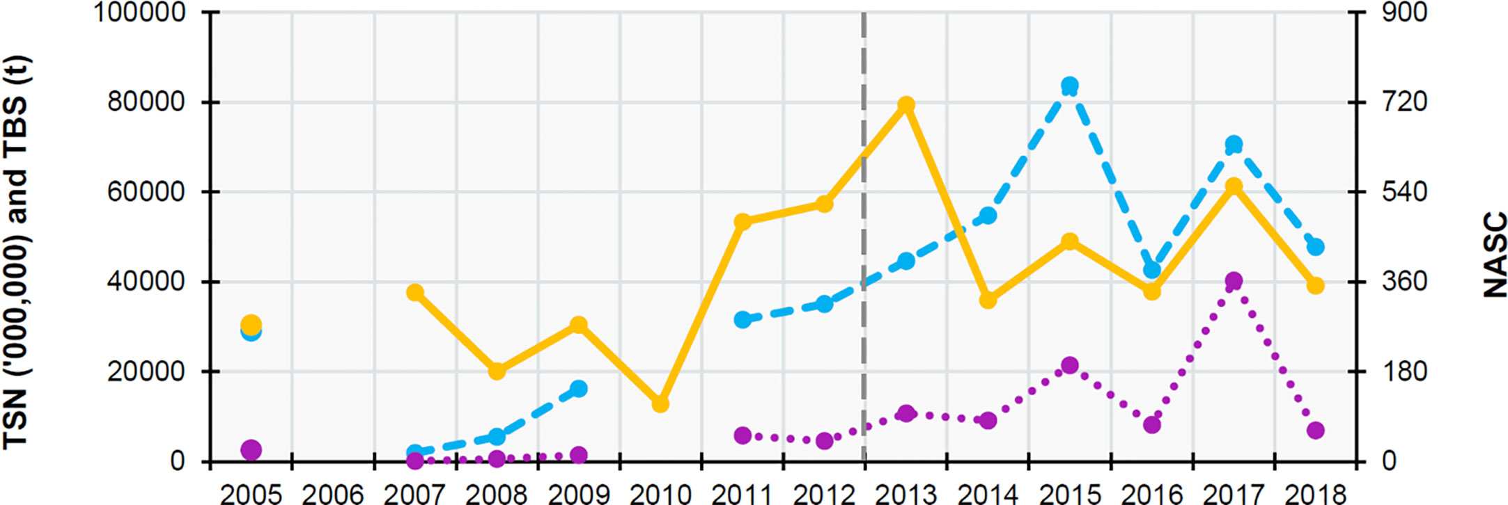
Figure 6 Time series graph representing the sprat (Sprattus sprattus) annual average values of the Total Stock Abundance (TSN, millions of fish, left axis; purple dotted line), Total Stock Biomass (TSB, t, left axis; blue dashed line),Nautical Area Scattering Coefficient (NASC, unitless, right axis; orange solid line) and year since the herring began to decline (dark grey dashed line). Data source: Annual Celtic Sea Herring Acoustic Surveys. Note the for 2006 there are no data and in 2010 TSN and TSB could not be calculated.

Common dolphins were the most abundant cetacean species recorded during the CSHASs, with an annual average of 911.6 ± 598.3 individuals recorded. Fin whales were the most frequently recorded baleen whale species, with an annual mean of 16 ± 13.5 individuals, which corresponds to approximately half of the average of all baleen whale species recorded, the latter group including fin, minke, humpback and unidentified baleen whales (30.6 ± 17.4 individuals).

The relative abundance of the three cetacean groups generally showed different year-to-year trends over the study period. The relative abundance in the area of common dolphins peaked in 2007 and 2016, while fin whales were most abundant in 2011 and the group of all baleen whales peaked in 2014 (Figure 7). However, all three groups showed similar trends during 2011-2015, with a low value in 2013 (the year in which herring abundance fell drastically).

FIGURE 7

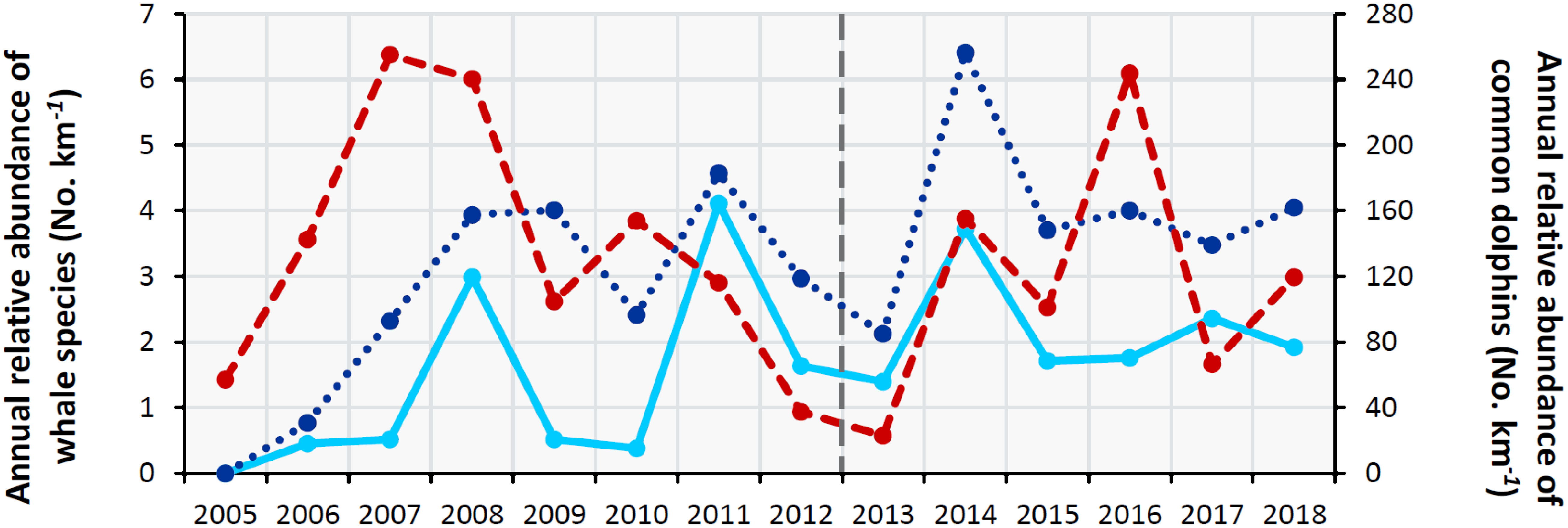
Figure 7 Time series graph of the annual number of individuals sighted standardized per km surveyed of each predator species. Common dolphin: red dashed line (right y-axis); sum of all baleen whale species: dark blue dotted line; fin whales: light blue solid line; year since the herring began to decline: dark grey dashed line. Data source: Annual Celtic Sea Herring Acoustic Surveys.

The distribution of the species changed between the periods before and since the decrease in the herring stock (Figures 2A, B and Supplementary Figure 2). The maps suggest that both prey and predator species have been more concentrated towards the south-eastern part of the study area since the herring decline. As previously commented the surveyed area was adjusted over time to account for the observed shift in herring spawning area. Herring density, as observed from survey data, showed a consistent decline year-on-year beginning in 2013, especially off the south and southwest coasts. Conversely, the maps suggest an increase in sprat density post-2013 off the southeast coast (Figure 2A). Predator abundance and distribution followed a similar pattern with an increase in abundance in the southeast and a decrease off the west coast. Maximum numbers of common dolphins were recorded off the southeast coast post-2013. In contrast, the highest concentrations of fin whales occurred pre-2013.

3.2 Modelling the environmental influence on prey

The presence of herring increased when increasing effort was applied and sea state worsens. Herring presence increased towards shallower waters and from the coastline up to 60km offshore (the trend for the latter variable was significant only relatively close to the coast; in deeper waters confidence limits were too wide to see a clear trend). Three dynamic oceanographic variables had a significant effect on the presence of herring. The presence of herring increased from the lowest PAR values up to 14 and also increased from values of -4 to -2 of the log-transformed standard deviation of chlorophyll concentration (logCHLSTD). The herring occurrence was inversely related to SST at temperatures higher than 14°C (Supplementary Figure 5A; Table 2B).

TABLE 2

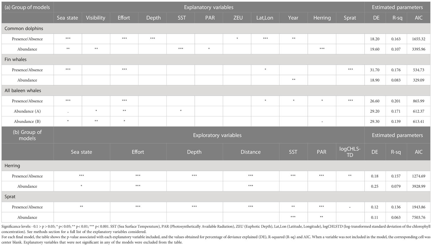
Table 2 Summary of the final binomial (presence) and negative binomial (abundance or acoustic density, where the species is present) models for (a) common dolphins, fin whales, all baleen whale species, (b) herring and sprat.

Where herring occurred, its acoustic density tended to be greater in shallower waters but also higher further from the shore. It should be borne in mind these are partial effects, i.e. at shorter distances from the shore density is higher if the water is shallower. The density also decreased from sea states 2 to 4 (Supplementary Figure 5B; Table 2B).

The presence of sprat increased when higher survey effort was applied and decreased from sea states 1 to 4. The presence of sprat was higher at medium distances from the shoreline and at medium depths. Sprat presence decreased as PAR increased up to a PAR value of 14 and increased for higher values of PAR. The presence of sprat increased significantly between 12.5°C and 14°C and decreased at higher temperatures. The effect of the log-transformed standard deviation of chlorophyll concentration was non-significant (p= 0.056) but including this variable improved the model (from an AIC value of 1947.41 to 1943.86). The presence of sprat showed a weak negative relationship with the variability of chlorophyll concentration (Supplementary Figure 6A; Table 2B).

The acoustic density of sprat (where present) was related to the same variables as in the presence model. Sprat density was negatively related to both SST (between 13°C and 15°C) and PAR (from PAR values of 13 to 16.5) (Supplementary Figure 6B; Table 2B). Validation tests for every prey model indicated no problems. For further details about the model selection process for herring and sprat, see Supplementary Tables 2, 3.

3.3 Modelling of cetacean distribution and abundance

3.3.1 Presence of common dolphins

The presence of common dolphins increased when higher survey effort occurred and sea state decreased. Based on visual examination of the smoother plots (Figure 8A), the effects of these variables became non-significant when survey effort was higher than 25km per cell and sea state was ≤1 or ≥4. From the contour plot, even though the probability of presence was quite high in southern waters, a coastal hot-spot occurred in the center of the study area. The presence of common dolphins fluctuated over the years, reaching a peak in 2016. Common dolphins were less likely to be present in the shallowest waters and occurrence increased towards deeper waters, up to approximately 80m. Over greater water depths, the trend became non-significant. The depth of the euphotic zone (ZEU) was the only dynamic oceanographic variable that showed a significant effect on common dolphin presence, with the highest probability of presence when ZEU was around 30m and decreasing as ZEU approached 40 m. Outside this range of ZEU values, the very wide confidence intervals mean that there was no clear significant trend. None of the prey species abundance indices showed a significant effect on the presence of this species (see Table 2A). For further details about the model selection process for the three groups of cetaceans species, see Supplementary Tables 4, 5.

FIGURE 8

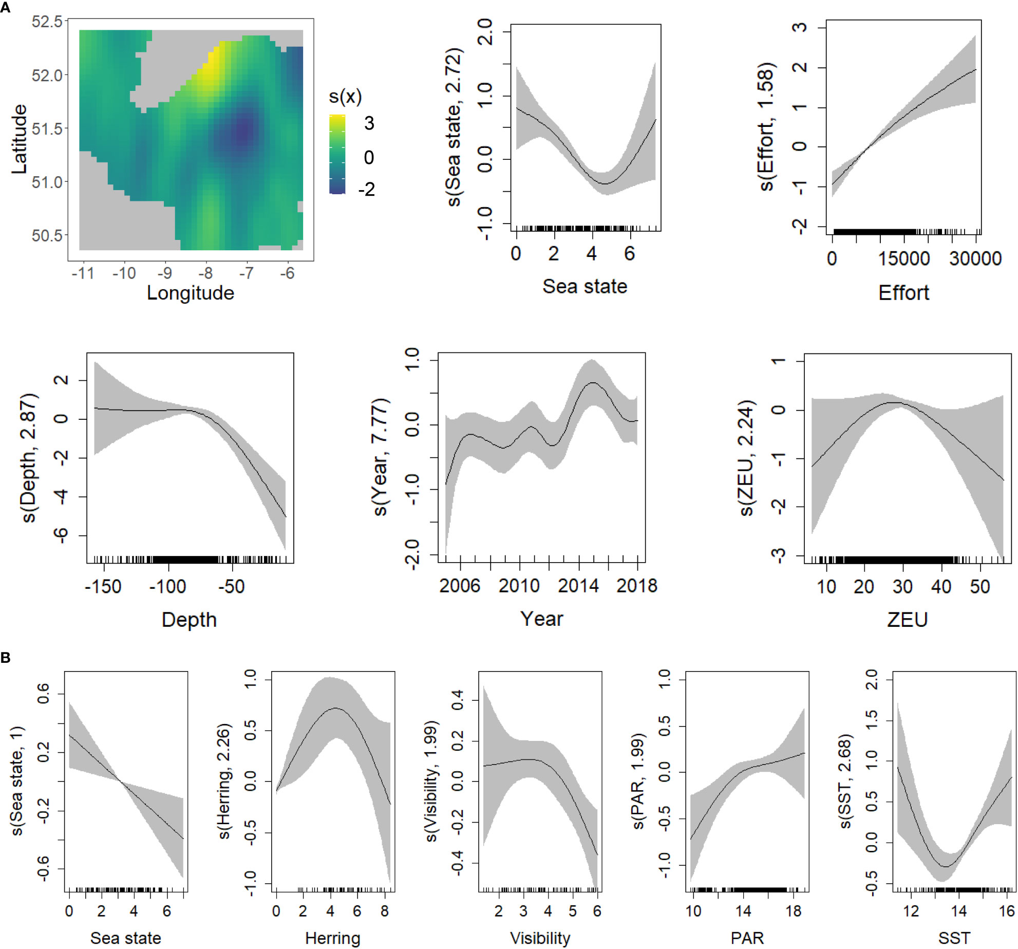
Figure 8 GAM smoothing curves for partial effects of the explanatory variables included in the final model of common dolphin presence (A) and abundance (B). The grey shaded area of the smoother plots corresponds to the 95% confidence intervals around the effect. In the top left corner (A), spatial variation in probability of presence of common dolphins is represented on a contour plot versus longitude (x axis) and latitude (y axis). (Note that the units on the Y axis of the smoother plots, and for colours on the contour plot, have not been transformed back to the original scale). ZEU (Euphotic Depth), PAR (Photosynthetically Available Radiation), SST (Sea Surface Temperature).

3.3.2 Abundance-given-presence of common dolphins

Where common dolphins were present, their abundance decreased when sea state increased and was lowest when visibility was highest. The abundance of this species (given presence) did not vary significantly over space and time once effects of other explanatory variables were considered. Abundance was lowest at around 13-14°C but increased in both colder and warmer waters. PAR had a weakly positive effect on common dolphin abundance. The trends associated with both oceanographic variables became non-significant towards the highest values. While there was significant spatio-temporal variation in the presence of this species, this was not the case for abundance-given-presence. Again, differing from the presence models, herring density showed a significant (but weak) effect on the number of common dolphins detected: dolphin abundance reached a peak at NASC values between 65-70 (i.e. log-transformed value of approximately 4.2) (Figure 8B; Table 2B).

3.3.3 Presence of fin whales

The presence of fin whales increased linearly with increasing survey effort and decreased linearly with increasing sea state. The occurrence of this species showed significant spatial variation, with a higher probability of presence close to the southwestern coast and in the center and south of the eastern part of the study area. Environmental conditions did not show any significant effects, but the presence of fin whales was positively related to sprat density (Figure 9A; Table 2A).

FIGURE 9

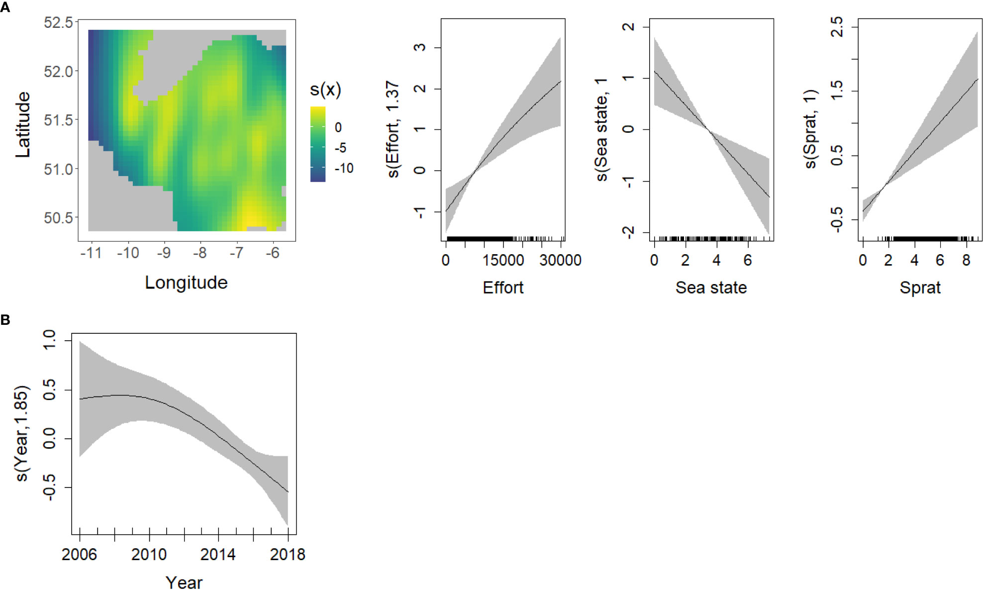
Figure 9 GAM smoothing curves fitted to partial effects of the explanatory variables included in the final model of fin whale presence (A) and abundance (B). Grey shaded areas of the smoother plots correspond to the 95% confidence intervals around the main effect. On the left, the spatial variation in probability of presence of fin whale is represented on a contour plot of the longitude (x axis) and latitude (y axis). (Note that the units on the Y axis of the smoother plots and for colours on the contour plot, have not been transformed back to the original scale).

3.3.4 Abundance-given-presence for fin whales

In the negative binomial models of the abundance of fin whales, only the effect of year was significant, with a decline in numbers over the last eight years of the study (Figure 9B; Table 2B).

3.3.5 Presence of all baleen whales

Similar to common dolphins, the occurrence of the “all baleen whales” category increased when more effort was applied and decreased as sea state increased. Mysticete species occurrence was highest in southwestern coastal areas and in the southeastern part of the study area. Their presence reached a maximum in 2015, although due to wide confidence intervals no significant trend is evident before 2014. Since 2015, the presence of baleen whales tended to decrease. Environmental conditions did not show any significant effect on the presence of baleen whales. Abundance of both prey species showed a positive linear effect on the presence of baleen whales, the effect being stronger in the case of sprat (deviance explained = 2.1% for sprat and 0.20% for herring) (Figure 10A; Table 2A).

FIGURE 10

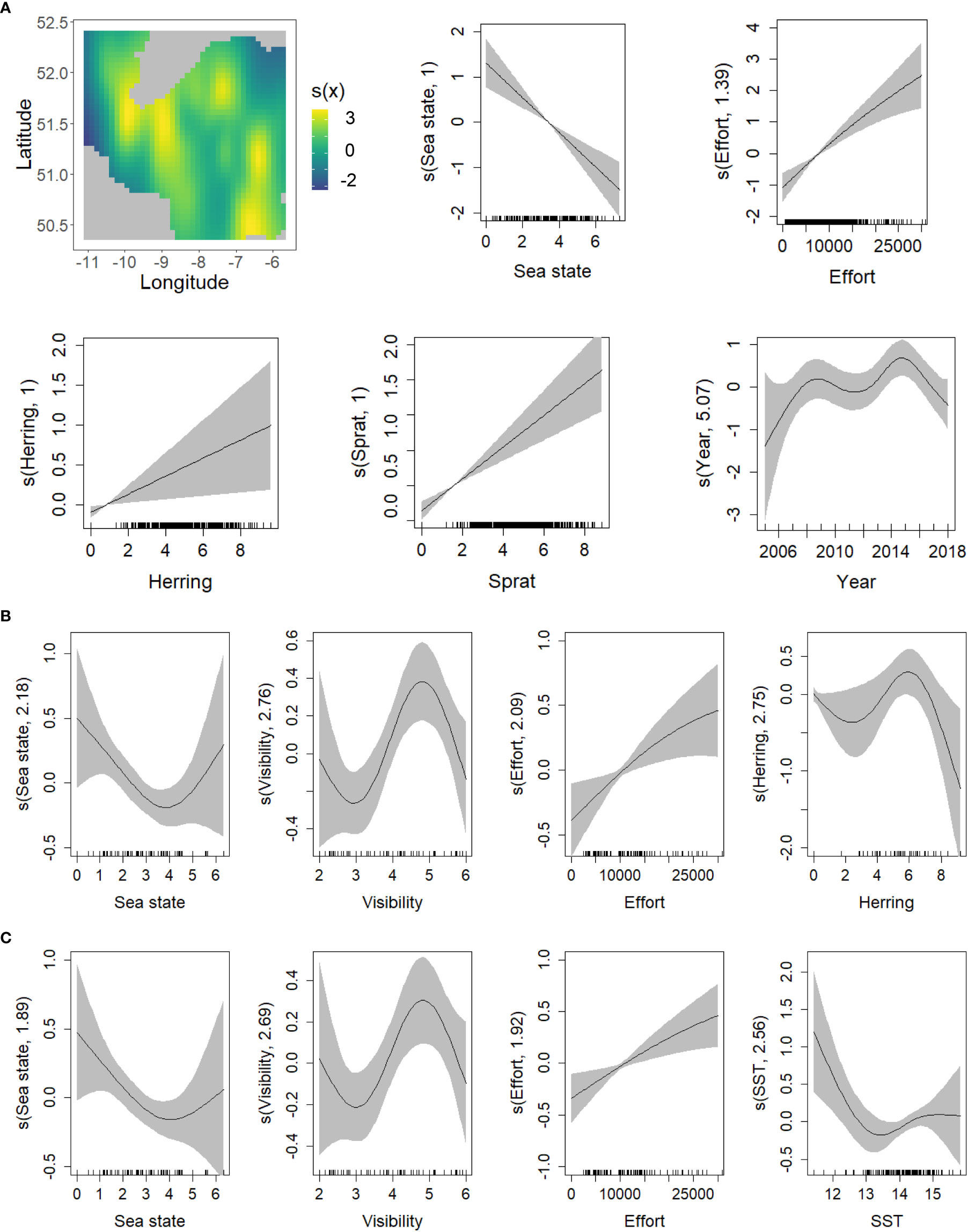
Figure 10 GAM smoothing curves for partial effects of the explanatory variables included in the final model of all baleen whale species presence (A) and abundance (B, C). The grey shaded area corresponds to the 95% confidence intervals around the main effect. In the top left corner (A), the spatial variation in probability of presence of whale species is represented on a contour plot of the longitude (x axis) and latitude (y axis). (Note that the units on the Y axis of the smoother plots and for colors on the contour plot, have not been transformed back to the original scale). SST (Sea Surface Temperature).

3.3.6 Abundance-given-presence for all baleen whales

Based on the criteria described, two final models were selected to explain the abundance of baleen whales, due to their similar performance (Model A: 29.2% DE, 612.37 AIC; Model B: 29.3% DE, 613.41 AIC). Both models included the three detectability variables (sea state, visibility and effort). Although the statistical significance of their effects differed between the two models, visually their partial effects were similar: the number of whales tended to fall from sea state 1 to 4, and increased with both increasing visibility (in the range 3 (6-10km) to 4.7 (13-14km)) and increasing survey effort. While model A also included SST, indicating that the most favorable SST for the abundance of whales was the coldest (11.5°C), model B included herring density and suggested a weak influence of herring density (p= 0.053), with peak whale abundance at intermediate densities and a marked decline in whale abundance at the highest NASC values. There was no significant spatiotemporal variation (Figures 10B, C; Table 2B). Validation tests for every cetacean model indicated no problems. For further details about the model selection process for common dolphins, fin whales and all whales, see Supplementary Tables 4, 5.

4 Discussion

The starting point for this study was the expectation that the changing status of the Celtic herring stock as revealed by annual acoustic surveys, has consequences for predators (including cetaceans) feeding on herring. By using a combination of fisheries acoustic and cetacean visual data from scientific surveys, we were able to investigate this potential shift. Changes in the environmental conditions associated with the herring stock decline were observed and the drivers of the presence and abundance of common cetaceans in the area were investigated, considering the roles of both environmental conditions and fish density. This study highlights the importance of prey availability in the distribution of cetaceans, which may be especially important in areas with high fishing pressure.

4.1 Herring decline and associated changes in ecosystem components

The Celtic Sea herring stock has collapsed three times during the last six decades (Clarke and Egan, 2017), most recently since 2013 accordingly to NASC data and derivate indicators (TSN and SSB) (O’Donnell et al., 2020) or since 2012 as suggested by the most recent stock assessment results (ICES, 2021b). Since then, the stock has also concentrated towards the south-eastern coastal and offshore waters of the study area where the last of the large aggregations are present. Herring has not been detected along the south-western coast in recent years. Consequently, fishing effort has also shifted to this area, followed by the CSHAS surveys (O’Donnell et al., 2020).

The lack of herring off the west coast suggests that the already declining autumn-western spawning ground (Harma et al., 2012: Volkenandt et al., 2014) has all but disappeared. Negative effects of increasing SST have been observed on the Celtic herring autumn-spawning grounds, favoring winter spawning (Haegele and Schweigert, 1985; Harma et al., 2012), reducing size-at-age in the Celtic Sea herring (Lyashevska et al., 2020) and decreasing productivity in Baltic herring (Moyano et al., 2020). Irish waters have had a warming trend between 1850 and 2007 (Cannaby and Hüsrevolu, 2009), leading to concern about the future of this stock (e.g. Harma et al., 2012), given the upper limit of the optimal temperature range of the species around 14°C (Volkenandt et al., 2014; Lyashevska et al., 2020). Although averaged SST in the study area did not increase significantly, it is clear from the oceanographic maps (Figure 4) that SST in the autumn spawning area did increase, which may support the hypothesis that the disappearance of the autumn-western spawning ground was also influenced by environmental change. However, other factors, such as the high fishing mortality, could have played a role as well.

Some fish stock collapses have been related to changes in environmental conditions which affect population parameters such as recruitment (e.g. Ottersen et al., 2010; Santos et al., 2012; Britten et al., 2016). In the Celtic Sea, no influence of changes in oceanographic conditions on herring distribution was found previous to the decline (Volkenandt et al., 2014). In contrast, our results from the data characterization suggested that some environmental changes could be associated with this herring decline, with SST increasing, CHL decreasing, and the ZEU extending deeper since 2013. These environmental changes were concentrated mainly in south-east and south-west coastal waters, the latter area coinciding with herring concentrations after the decline and the autumn spawning grounds (O’Sullivan et al., 2013). The prey models indicated that the probability of herring presence decreased for SSTs higher than 14°C. These models also showed an increasing trend of herring occurrence associated with increasing PAR (a primary productivity proxy), up to medium values of PAR of 14. Herring presence also increased with higher values of logCHLSTD (at least within the mid-range of logCHLSTD values).

In contrast to herring, sprat biomass increased over the study period. Other studies have shown that herring and sprat respond differently to changes in environmental conditions (e.g. Hunter et al., 2019). The prey models revealed that the same variables that affected herring presence, also affect sprat but in different ways. Their acoustic density where they were present was driven by the static environmental variables (depth and distance to the coast) in the case of herring, and by the dynamic variables (PAR and SST) for sprat.

It might be expected that these changes in the Celtic Sea ecosystem would also affect predators of herring (Surma et al., 2018). No clear temporal association was evident between the time series of the relative abundance of cetaceans and prey density. First of all, absolute abundance of cetacean populations is unlikely to show an immediate response to changing prey abundance, even for preferred prey (any such changes would be slow due to the long generation times of cetaceans). It is more plausible that local abundance of cetaceans would track local abundance of important prey, but whether this could be detected depends on the extent of the change and on the scale at which it occurs, relative to the scale of the analysis. It should also be highlighted that the number of cetacean sightings was at the minimum values of the time series for all species, especially common dolphins, for which the number of sightings reached its lowest value in 2013, when the herring began to decline. Over the area, the distribution of the study species has showed similarities since 2013 when the highest relative abundances of cetaceans and herring were seen in the same two hot-spots. When humpback, minke and unidentified whales are considered together with fin whales, even though these rorqual species occurred at the herring hot-spots, their occurrence was also more widespread, consistent with differences in prey-predator associations among the rorqual species, as suggested by Volkenandt et al. (2015).

4.2 Drivers of the relative abundance and distribution of common dolphins in the study area

Brophy et al. (2009) found that herring and sprat were minor components of the diet of common dolphins (stranded and bycaught individuals) in the Celtic Sea. Despite this, our results indicated that where these dolphins were present, their local relative abundance increased as herring densities increased from low to medium values. In addition, the minimum number of common dolphins occurred in 2013, prior to the most recent herring decline. The positive effect of increasing herring density is however consistent with the previously reported preference of common dolphins for energy-rich small pelagic species such as sardines, anchovies (Engraulis encrasicolus), mackerel (Scomber scombrus), sprat and herring, observed in several different regions and populations (e.g. Silva, 1999; Meynier et al., 2008; Pierce et al., 2008; Spitz et al., 2010; Santos et al., 2013). The apparent differences between our model results and what might have been expected from common dolphin diet, as described in the area by Brophy et al. (2009), could be due to high herring densities being associated with high prey availability generally - with the dolphins feeding on other prey species - or may indicate that the local importance of herring in common dolphin diet in recent years has been higher than was generally the case in the Celtic Sea.

Habitat use by common dolphins in the study area appears to be characterized by certain environmental conditions (bearing in mind that this possible preference may be secondary, related to the habitat preferences of their prey). Our results suggest that common dolphins were most likely to be present in coastal areas, in intermediate water depths (approximately 80 m) where the euphotic layer extends to around 30m. A preference for shallower or intermediate depths and coastal waters elsewhere has been related to prey distribution (Cañadas and Hammond, 2008; Silva et al., 2014; Tobeña et al., 2016; Milani and Vella, 2019).

Where common dolphins were present in the study area, they were more abundant in the coldest and the warmest waters registered during the study period, with lowest abundance in the range 12.5-14°C. Different theories about the relationships of this species with SST have been described elsewhere. For example, associations of common dolphins with warm waters have been observed in Irish and British waters (MacLeod et al., 2008: Robinson et al., 2010), while a thermal niche model suggested sea temperatures below 14°C were less suitable for common dolphins in the northeast Atlantic (Lambert et al., 2011). However, common dolphins may occur in colder waters due to high local productivity resulting from upwelling (Cañadas and Hammond, 2008; Correia et al., 2019). Local and seasonal upwelling events, highly variable in periodicity and magnitude, take place in Irish waters which affect the phytoplankton community and may have an effect on the food web, up to top predators (Raine et al., 1993; Edwards et al., 1996; O’Boyle et al., 2009).

In the present study, local abundance of common dolphins in the region increased towards areas with higher values of the primary production proxy PAR but the other primary production proxies used in the analysis (CHL and ZEU) did not have a significant effect. This apparent discrepancy could be explained by the time-lags associated with the effects of both proxies. The use of electromagnetic radiation as a source of energy for photosynthesis (PAR) needs time (Mõttus et al., 2012), and it also takes time for the effects to work their way through the food chain to top predators. Time-lags between CHL peaks and peaks of abundance of common dolphins have been already described, e.g. in the Azores (Tobeña et al., 2016). Evidently, caution is needed when interpreting effects inferred from statistical modelling of habitat preferences since the models are a fairly simplistic representation of what can be very complex processes.

4.3 Drivers of the relative abundance and distribution of whales in the study area

Baleen whales (rorquals) feed primarily on krill and small schooling fish such as herring and sprat, and occasionally on squids (Kawamura, 1980; Barros and Clarke, 2009). The diet composition varies among rorqual species as well as by area and season. The three rorqual species analyzed in this study have been shown to change their diet according to the season and location, related to prey availability (e.g. Witteveen et al., 2012; Víkingsson et al., 2014; Nøttestad et al., 2015; Aguilar and García-Vernet, 2018).

The results of the models showed a positive effect of sprat density on the presence of both rorqual species groups analyzed (i.e. fin whales and all baleen whales). Sprat density was one of the two factors that affected the local abundance of these whale species where they were present (although the nature of the relationship was not as expected: baleen whales were more abundant at intermediate herring densities). Herring density had a weak (compared to the effect of sprat density) but significantly positive effect on the presence of the all baleen whales group. Fin whale presence was not affected by herring density.

The differences found between the two groups (i.e. fin whales and all baleen whales) suggest that minke, humpback and/or other unidentified whale species may have relied more on herring than was the case for fin whales. Previous research using stable isotope composition of skin samples suggested differences in the diet of fin and humpback whales in the study area, with krill being more important in the diet of fin whales, while small herring and large sprat were more important for humpback whales (Ryan et al., 2013a). Evidence of fin whales feeding on krill in offshore waters off the west of our study area (i.e. Porcupine Seabight) was also found by Baines et al. (2017). Fin whales were the most frequently sighted and abundant baleen whale species in the study area and, based on this information the least likely to be affected by changes in herring abundance; the effect of herring abundance on the presence of the all baleen whales group is thus most likely due to effects on the other rorqual species present. Evidently, it would be useful to have information on krill density in the study area.

Results from the models showed a significant decrease in the abundance of fin whales where they were present since 2013 (although there was no significant change in the proportion of presence records), agreeing with the decrease in the total number of sightings of this species reported in Irish inshore waters during April to August, from 517 sightings in 2008 to 190 in 2018 by Whooley (2019), which is also consistent with unpublished data held by IWDG (Simon Berrow and Dave Wall, Personal observation, 12^th August 2019). No clear trend was observed from the time series on the number of sightings divided by effort of fin whales in the study area. Note that the annual average sightings rate is a function of both the proportion of presences and the abundance where the animals are present. Our models showed no effect of herring density on fin whales but there was a direct relationship with sprat (i.e. fin whales presence increased with higher sprat density).

Of the environmental factors considered, only SST showed an effect on the abundance of the baleen whale group in the study area. Baleen whales in general seemed to be more abundant in the coldest areas and, as also seen in common dolphins, less numerous in temperatures from 12.5 to 14°C. This raises the question of whether the lower abundance of cetaceans in this SST range is a direct effect of SST or an indirect consequence of its effect on fish abundance (as discussed in the previous section).

4.4 Limitations

Multiannual ecosystem surveys, such as the CSHAS, in principle can overcome the common limitations such as the lack of spatio-temporal consistency and lack of simultaneously recorded data from different taxa or ecosystem variables (Torres et al., 2008). However, the data refer to a specific time of year (October) and in a specific area, so that effects with a time-lag of less than one year and events which occur in surrounding waters are hidden from the study. Moreover, in most real world situations prey availability in the moment and area where a sighted cetacean is feeding is hard to measure, and it is therefore difficult to determine whether foraging choices are truly opportunistic (Torres et al., 2008; Santos et al., 2013), and consequently, we cannot be sure how cetaceans perceive prey availability. The fine-scale resolution of the available acoustic raw data (NASC, 1.85km) allowed the interpretation of prey-predator associations. However, even though NASC was used as a proxy of fish abundance, it should be kept in mind that NASC measures the acoustic density of the fish, which may also be affected by other factors such as the size of the species or migration behavior which might influence their target strength (Simmonds and Maclennan, 2007).Visual data on cetaceans have some unavoidable limitations, including the use of multiple observers with different levels of experience contributing to long-term datasets and detection bias since sightings are only possible when the animals are at the surface. In the present study, an additional issue was the use of a different platform during very poor weather (i.e. when the weather was rougher the observers needed to come down from the crow’s nest to the bridge). Because this change in platform height was associated with rougher weather, we expect that most of the effect of this change will have been included in the explanatory variable sea state. Although fishery surveys typically following a transect-based design which in principle enables the estimation of marine mammal abundance through distance sampling (Buckland et al., 1993), the CSHAS design did not follow the requirements (e.g. two observer platforms would be needed). Consequently, we could not calculate a detection function nor estimate the proportion of animals not seen due to being underwater (g(0)), even though it was possible to model the effects of environmental conditions on sightings detection probability. Thus, the number of sighted cetaceans per km on effort, is at best a measure of relative abundance of cetaceans.

The results of the models might be improved by accounting for additional variables that affect the detection probability of cetaceans, such as swell, glare, precipitation, etc. This information was not consistently recorded throughout the study period and could not be used. The resolution of fin and baleen whale models could be improved by using a larger number of observations of these species, such as might become available if the work continues for several more years. Moreover, testing the effects of other variables such as NAO, intensity of the currents and the wind, and considering time-lagged effects of variables, could contribute to achieve a better understating of how environmental variables affect the relative abundance and distribution of cetaceans.

It is important to point out that even though we had 14 years of data to fit the GAMs, with larger number of observations it is preferable to divide data into “model fitting” and “model testing” components. Predictions derived from the former can be tested against the latter, thus allowing a genuine hypothesis test. Results from GAMs (or indeed other kinds of statistical models) fitted to entire datasets are best viewed as descriptive, representing a hypothesis that still needs to be tested. Statistical correlation cannot be used to prove the existence of cause-effect relationships.

Better understanding of the system studied is essential to allow correct interpretation of the results. For example, complementary studies of the feeding ecology of the cetaceans based on stable isotope analysis of tissue samples would be useful.

5 Conclusions

The Celtic Sea herring stock suffered a marked decline since 2013. From then, the stock has concentrated during October towards the south-eastern coastal and southern offshore Irish waters within the Celtic Sea ecoregion. In the same period sprat density increased, the sea surface temperature increased, chlorophyll concentration decreased and the euphotic zone extended to greater depths. The models for herring and sprat support the idea that these species have different environmental relationships.

The factors influencing the probability of presence and relative abundance of the cetaceans differed between species. The presence of common dolphins was related to depth while, where they were present, their abundance was related to SST and herring density. Fin whales were more likely to be present where there was a higher density of sprat, while when all whale species were considered, there was also an effect of herring density. Where present, abundance of all whale species was related to warmer sea surface waters and herring density.

The results obtained provide valuable information about the functioning of the Celtic Sea ecosystem and the distribution and feeding ecology of cetaceans, as well as describing changes associated with the decline of the herring stock. They are potentially relevant for the implementation of the MSFD, specifically of the Descriptors 1, 3 and 4 (Biodiversity, Population of commercial fish species and Food webs, respectively). In addition, understanding the complex and dynamic relationships among different ecosystem components (predators, prey and the environment) can inform the implementation of Ecosystem-Based Management. Lastly, the work highlights the benefits of carrying out integrative surveys in which information about different ecosystem components is gathered simultaneously.

Data availability statement

The data analyzed in this study is subject to the following licenses/restrictions: The raw datasets of fish and cetacean species analyzed for this study are subject to data requests to the Marine Institute and the Irish Whale and Dolphin Group. Requests to access these datasets should be directed to corresponding author and co-authors, https://www.marine.ie/marine-institute-request-digital-data, https://iwdg.ie/access-to-iwdg-sighting-and-stranding-data/.

Ethics statement

Ethical review and approval was not required for the animal study because this research is based on data from observations (cetaceans sightings and acoustic fisheries data) without applying any techniques that might disturb the animals.

Author contributions

SB and AF-B designed the research. CO’D, SB, DW, VV, MG, and AF-B collected data. AF-B and GP analyzed the data. All the authors contributed to the study with ideas and knowledge and to write up the manuscript.

Funding

Cetacean data collected by the IWDG was part-funded by the Heritage Council, the National Parks and Wildlife Service of the Department of Housing, Local Government and Heritage, and the Marine Institute under various funding streams including Marine Mammals and Megafauna in Irish Waters – Behaviour, Distribution and Habitat Use. Marine Research Sub-programme (PBA/ME/07/005(2)).

Acknowledgments

We are grateful to the crew and teams of Marine Mammal Observers and fishery acousticians who contributed to the collection and processing of data from the annual Celtic Sea Herring Acoustic Surveys. We thank the members of the Department of Ecology and Marine Resources at the IIM-CSIC, also Begoña Santos and Camilo Saavedra, for their helpful contributions and valuable discussions concerning data analysis and interpretation. We are grateful to the Marine Institute and the Irish Whale and Dolphin Group for providing the data.

Conflict of interest

The authors declare that the research was conducted in the absence of any commercial or financial relationships that could be construed as a potential conflict of interest.

Publisher’s note

All claims expressed in this article are solely those of the authors and do not necessarily represent those of their affiliated organizations, or those of the publisher, the editors and the reviewers. Any product that may be evaluated in this article, or claim that may be made by its manufacturer, is not guaranteed or endorsed by the publisher.

Supplementary material

The Supplementary Material for this article can be found online at: https://www.frontiersin.org/articles/10.3389/fmars.2023.1033758/full#supplementary-material

References

Aguilar A., García-Vernet R. (2018). “Fin whale: balaenoptera physalus,” in Encyclopedia of marine mammals (London: Academic Press), 368–371.

Google Scholar

Anderson D. R., Burnham K. P. (2002). Avoiding pitfalls when using information-theoretic methods. J. Wildlife Manage. 66 (3), 912–918. doi: 10.2307/3803155

CrossRef Full Text | Google Scholar

Anderwald P., Evans P. G. H., Dyer R., Dale A., Wright P. J., Hoelzel A. R. (2012). Spatial scale and environmental determinants in minke whale habitat use and foraging. Mar. Ecol. Prog. Ser. 450, 259–274. doi: 10.3354/meps09573

CrossRef Full Text | Google Scholar

Baines M., Reichelt M., Griffin D. (2017). An autumn aggregation of fin (Balaenoptera physalus) and blue whales (B. musculus) in the porcupine seabight, southwest of Ireland. Deep-Sea Res. Part II: Topical Stud. Oceanography 141, 168–177. doi: 10.1016/j.dsr2.2017.03.007

CrossRef Full Text | Google Scholar

Barros N. B., Clarke M. R. (2009). “Diet,” in Encyclopedia of marine mammals (London: Academic Press), 311–316.

Google Scholar

Barlow J. (2015). Inferring trackline detection probabilities, g (0), for cetaceans from apparent densities in different survey conditions. Mar. Mammal Sci. 31 (3), 923–943. doi: 10.1111/mms.12205

CrossRef Full Text | Google Scholar

Britten G. L., Dowd M., Worm B. (2016). Changing recruitment capacity in global fish stocks. Proc. Natl. Acad. Sci. 113 (1), 134–139. doi: 10.1073/pnas.1504709112

CrossRef Full Text | Google Scholar

Brophy J. T., Murphy S., Rogan E. (2009). The diet and feeding ecology of the short-beaked common dolphin (Delphinus delphis) in the northeast Atlantic. Reports of the International Whaling Commission, SC/61/SM 14.

Google Scholar

Brunel T., Dickey-collas M. (2010). Effects of temperature and population density on von bertalanffy growth parameters in Atlantic herring: a macro-ecological analysis. Mar. Ecol. Prog. Ser. 405, 15–28. doi: 10.3354/meps08491

CrossRef Full Text | Google Scholar

Buckland S. T., Anderson D. R., Burnham K. P., Laake J. L. (1993). Distance sampling: estimating abundance of biological populations (London: Chapman and Hall), 446.

Google Scholar

Cannaby H., Hüsrevolu Y. S. (2009). The influence of low-frequency variability and long-term trends in north Atlantic sea surface temperature on irish waters. ICES J. Mar. Sci. 66 (7), 1480–1489. doi: 10.1093/icesjms/fsp062

CrossRef Full Text | Google Scholar

Cañadas A., Hammond P. S. (2008). Abundance and habitat preferences of the short-beaked common dolphin delphinus delphis in the southwestern Mediterranean: implications for conservation. Endangered Species Res. 4 (3), 309–331. doi: 10.3354/esr00073

CrossRef Full Text | Google Scholar

Cardinale M., Cardinale M., Casini M., Arrhenius F., Håkansson N. (2003). Diel spatial distribution and feeding activity of herring (Clupea harengus) and sprat (Sprattus sprattus) in the Baltic Sea. Aquat. Living Resour. 16 (3), 283–292. doi: 10.1016/S0990-7440(03)00007-X

CrossRef Full Text | Google Scholar

Carvalho N., Keatinge M., Guillen Garcia J. EUR 28359 EN (Luxembourg: Publications Office of the European Union). doi: 10.2760/911768

CrossRef Full Text | Google Scholar

Castro J., Couto A., Borges F. O., Cid A., Laborde M. I., Pearson H. C. (2020). Oceanographic determinants of the abundance of common dolphins (Delphinus delphis) in the south of Portugal. Oceans 1 (3), 165–173. doi: 10.3390/oceans1030012

CrossRef Full Text | Google Scholar

Clarke M., Egan A. (2017). Good luck or good governance? the recovery of celtic Sea herring. Mar. Policy 78 (September 2016), 163–170. doi: 10.1016/j.marpol.2016.10.025

CrossRef Full Text | Google Scholar

Correia A. M., Gil Á., Valente R., Rosso M., Pierce G. J., Sousa-pinto I. (2019). Distribution and habitat modelling of common dolphins (Delphinus delphis) in the eastern north Atlantic. J. Mar. Biol. Assoc. United Kingdom 99, 1443–1457. doi: 10.1017/S0025315419000249

CrossRef Full Text | Google Scholar

Council Directive 92/43/EEC (1992). Of 21 may 1992 on the conservation of natural habitats and of wild fauna and flora. OJ l 206/7. Off. J. Eur. Union L206, 7–50.

Google Scholar

Cragg J. G. (1971). Some statistical models for limited dependent variables with application to the demand for durable goods. Econometrica 39, 829–844. doi: 10.2307/1909582

CrossRef Full Text | Google Scholar

CSHMAC (2018). “Report no MSC026,” in Marine stewardship council full re-assessment public certification report for the CSHMAC (Celtic Sea herring management advisory committee) celtic Sea herring fishery, SAI global.

Google Scholar

Derville S., Torres L. G., Iovan C., Garrigue C. (2018). Finding the right fit: comparative cetacean distribution models using multiple data sources and statistical approaches. Diversity Distributions 24), 1657–1673. doi: 10.1111/ddi.12782

CrossRef Full Text | Google Scholar

Directive 2008/56/EC (2008). Of the European parliament and of the council of 17 June 2008 establishing a framework for community action in the field of marine environmental policy (Marine strategy framework directive). OJ l 164/19. Off. J. Eur. Union L164, 19–40.

Google Scholar

Edwards A., Jones K., Graham J. M., Griffiths C. R., MacDougall N., Patching J., et al. (1996). Transient coastal upwelling and water circulation in bantry bay, a ria on the south-west coast of Ireland. Estuarine Coast. Shelf Sci. 42 (2), 213–230. doi: 10.1006/ecss.1996.0016

CrossRef Full Text | Google Scholar

Engelhard G. H., Peck M. A., Rindorf A., Smout C. S., van Deurs M., Raab K., et al. (2014). Forage fish, their fisheries, and their predators: who drives whom? ICES J. Mar. Sci. 71 (1), 90–104. doi: 10.1093/icesjms/fst087

CrossRef Full Text | Google Scholar

Eurostat (2020) Fish catch 2019. Available at: https://ec.europa.eu/eurostat/web/products-eurostat-news/-/edn-20201016-3 (Accessed 13 November 2021).

Google Scholar

ESRI (2011). ArcGIS desktop: release 10 (Redlands, CA: Environmental Systems Research Institute).

Google Scholar

ESRI (2016). ArcGIS desktop: release 10.4 (Redlands, CA: Environmental Systems Research Institute Ì).

Google Scholar

Forney K. (2000). Environmental models of cetacean abundance: reducing uncertainty in population trends. Conserv. Biol. 14, 1271–1286. doi: 10.1046/j.1523-1739.2000.99412.x

CrossRef Full Text | Google Scholar

Gannier A. (2002). Summer distribution of fin whales (Balaenoptera physalus) in the northwestern Mediterranean marine mammals sanctuary. Rev. d’Ecologie (La Terre la Vie) 57 (2), 135–150. doi: 10.3406/revec.2002.2390

CrossRef Full Text | Google Scholar

Gerritsen H. D., Lordan C. (2014). Atlas of commercial fisheries around Ireland (Ireland: Marine Insitute), 59. Available at: http://hdl.handle.net/10793/958.

Google Scholar

González García L., Pierce G. J., Autret E., Torres-Palenzuela J. M. (2018). Multi-scale habitat preference analyses for azorean blue whales. PloS One 13 (9), e0201786. doi: 10.1371/journal.pone.0201786

PubMed Abstract | CrossRef Full Text | Google Scholar

Haegele C. W., Schweigert J. F. (1985). Session 2: spawning, development, and survival of early life stages of herring distribution and characteristics herring spawning grounds and description of spawning behavior. Can. J. Fisheries Aquat. Sci. 42, 39–55. doi: 10.1139/f85-261

CrossRef Full Text | Google Scholar

Harma C., Brophy D., Minto C., Clarke M. (2012). The rise and fall of autumn-spawning herring (Clupea harengus l.) in the celtic Sea between 1959 and 2009: temporal trends in spawning component diversity. Fisheries Res. 121–122, 31–42. doi: 10.1016/j.fishres.2012.01.005

CrossRef Full Text | Google Scholar

Hunter A., Speirs D. C., Heath M. R. (2019). Population density and temperature correlate with long-term trends in somatic growth rates and maturation schedules of herring and sprat. PloS One 14 (3). doi: 10.1371/journal.pone.0212176

CrossRef Full Text | Google Scholar

ICES (2017). “Sprat (Sprattus sprattus) in subarea 6 and divisions 7.a–c and 7.f–k (West of Scotland, southern celtic seas),” in Report of the ICES advisory committee 2017, vol. 2017. (ICES Advice). doi: 10.17895/ices.pub.3258

CrossRef Full Text | Google Scholar

ICES (2018a). “Herring (Clupea harengus) in divisions 7.a south of 52°30’N, 7.g–h, and 7.j–k (Irish Sea, celtic Sea, and southwest of Ireland),” in Report of the ICES advisory committee 2018, vol. 2018. (ICES Advice). doi: 10.17895/ices.pub.4475/

CrossRef Full Text | Google Scholar

ICES (2018b). ‘Report of the workshop on integrated trend analysis in support to integrated ecosystem assessment (WKINTRA)’, (Hamburg, Germany: ICES CM 2018/IEASG) 14, 21.

Google Scholar

ICES (2019). ‘EU request for advice on a monitoring TAC for herring in ICES divisions 7 . a south of 52 ° 30 ‘ n , 7 . g – h , and 7 . j – k’, in report of the ICES advisory committee 2019 Vol. 2019 (ICES Advice). doi: 10.17895/ices.advice.5614

CrossRef Full Text | Google Scholar

ICES (2020a). Herring (Clupea harengus) in divisions 7.a south of 52°30’N, 7.g–h, and 7.j–k (Irish Sea, celtic Sea, and southwest of Ireland) Vol. 2020 (Report of the ICES Advisory Committee). doi: 10.17895/ices.advice.5944

CrossRef Full Text | Google Scholar

ICES (2020b). Herring assessment working group for the area south of 62° n (HAWG) Vol. 2 (ICES Scientific Reports), 1151. doi: 10.17895/ices.pub.6105

CrossRef Full Text | Google Scholar

ICES (2021a). Herring (Clupea harengus) in divisions 7.a south of 52°30’N, 7.g-h, and 7.j-k (Irish Sea, celtic Sea, and southwest of Ireland) (ICES Advisory Committee). doi: 10.17895/ices.advice.7773

CrossRef Full Text | Google Scholar

ICES (2021b). Herring assessment working group for the area south of 62° n (HAWG) Vol. 3 (ICES Scientific Reports), 779. doi: 10.17895/ices.pub.8214

CrossRef Full Text | Google Scholar

IFAW (2000). Logger 2000 software (London: International Fund for Animal Welfare).

Google Scholar

Kawamura A. (1980). A review of food of balaenopterid whales. Sci. Rep. Whales Res. Inst. 32), 155–197.

Google Scholar

Lambert E., MacLeod C. D., Hall K., Brereton T., Dunn T. E., Wall D., et al. (2011). Quantifying likely cetacean range shifts in response to global climatic change: implications for conservation strategies in a changing world. Endangered Species Res. 15 (3), 205–222. doi: 10.3354/esr00376

CrossRef Full Text | Google Scholar

Lambert C., Mannocci L., Lehodey P., Ridoux V. (2014). Predicting cetacean habitats from their energetic needs and the distribution of their prey in two contrasted tropical regions. PloS One 9 (8), e0105958. doi: 10.1371/journal.pone.0105958

CrossRef Full Text | Google Scholar

Lambert C., Authier M., Doray M., Dore G., Ridoux V. (2018). Hide and seek in the bay of Biscay {{/amp]]mdash; a functional investigation of marine megafauna and small pelagic fish interactions. ICES J. Mar. Sci. 76 (1), 113–123. doi: 10.1093/icesjms/fsy143

CrossRef Full Text | Google Scholar

Lyashevska O., Harma C., Minto C., Clarke M., Brophy D. (2020). Long-term trends in herring growth primarily linked to temperature by gradient boosting regression trees. Ecol. Inf. 60 (April), 101154. doi: 10.1016/j.ecoinf.2020.101154

CrossRef Full Text | Google Scholar

MacLeod C. D. (2013). An introduction to using GIS in marine biology (Glasgow: Pictish Beast Publications).

Google Scholar

Macleod K., Fairbairns R., Gill A., Fairbairns B., Gordon J., Blair-Myers C., et al. (2004). Seasonal distribution of minke whales balaenoptera acutorostrata in relation to physiography and prey off the isle of mull, Scotland. Mar. Ecol. Prog. Ser. 277, 263–274. doi: 10.3354/meps277263

CrossRef Full Text | Google Scholar

MacLeod C. D., Weir C. R., Santos M. B., Dunn T. E. (2008). Temperature-based summer habitat partitioning between white-beaked and common dolphins around the united kingdom and republic of Ireland. J. Mar. Biol. Assoc. United Kingdom 88 (6), 1193–1198. doi: 10.1017/S002531540800074X

CrossRef Full Text | Google Scholar

Marine Institute (2013). The stock book 2013: annual review of fish stocks in 2013 with management advice for 2014 (Rinville, Oranmore, Ireland: Marine Institute).

Google Scholar

Meynier L., Pusineri C., Spitz J., Santos M. B., Pierce G. J., Ridoux V., et al. (2008). Intraspecific dietary variation in the short-beaked common dolphin delphinus delphis in the bay of Biscay: importance of fat fish. Mar. Ecol. Prog. Ser. 354, 277–287. doi: 10.3354/meps07246

CrossRef Full Text | Google Scholar

Milani C., Vella A. (2019). Abundance , distribution and diet of the common dolphin , delphinus delphis , in the northern Aegean Sea ( Greece ). Aquatic Conserv: Mar. Freshw. Ecosyst. 1–11. doi: 10.1002/aqc.3081

CrossRef Full Text | Google Scholar

Molloy J. (2006). The herring fisheries of Ireland 1900–2005: biology, research, development and assessment (Rinville, Oranmore, Ireland: Marine Institute).

Google Scholar

Mõttus M., Sulev M., Baret F., Lopez-Lozano R., Reinart A. (2012). “Photosynthetically active radiation: measurement and modeling,” in Encyclopedia of sustainability science and technology. Ed. Meyers (New York, NY: Springer). doi: 10.1007/978-1-4614-5806-7_451

CrossRef Full Text | Google Scholar

Moyano M., Illing B., Polte P., Kotterba P., Zablotski Y., Gröhsler T., et al. (2020). Linking individual physiological indicators to the productivity of fish populations: a case study of Atlantic herring. Ecol. Indic. 113, 106146. doi: 10.1016/j.ecolind.2020.106146

CrossRef Full Text | Google Scholar

Nøttestad L., Krafft B. A., Anthonypillai V., Bernasconi M., Langård L. (2015). Recent changes in distribution and relative abundance of cetaceans in the Norwegian Sea and their relationship with potential prey. Front. Ecol. Evol. 2 (83). doi: 10.7557/3.2713

CrossRef Full Text | Google Scholar

O’Boyle S., McDermott G., Wilkes R. (2009). Dissolved oxygen levels in estuarine and coastal waters around Ireland. Mar. Pollut. Bull. 58 (11), 1657–1663. doi: 10.1016/j.marpolbul.2009.07.002

PubMed Abstract | CrossRef Full Text | Google Scholar

O’Brien J., Berrow S., McGrath D., Evans P. (2009). Cetaceans in irish waters: a review of recent research. Biol. Environ. 109 (2), 63–88. doi: 10.3318/BIOE.2009.109.2.63

CrossRef Full Text | Google Scholar

O’Donnell C., Mullins E., Lynch D., Lyons K., Keogh N., Callaghan S. O., et al. (2018). Celtic Sea herring acoustic survey cruise report 2018, 8-28 October 2018 Vol. 2018 (Marine Institute).

Google Scholar

O’Donnell C., Mullins E., Lyons K., Connaughton P., Perez Tadeo M. (2020). Celtic Sea herring acoustic survey cruise report 2020, 4-24 October 2020 Vol. 2020 (Marine Institute).

Google Scholar

O’Sullivan D., O’Keeffe E., Berry A., Tully O., Clarke M. (2013). An inventory of Irish herring spawning grounds. Irish Fisheries Bull. 42, 38.

Google Scholar

Ottersen G., Kim S., Huse G., Polovina J., Stenseth N. C. (2010). Major pathways by which climate may force marine fish populations. J. Mar. Syst. 79, 343–360. doi: 10.1016/j.jmarsys.2008.12.013

CrossRef Full Text | Google Scholar

Palialexis A., Connor D., Damalas D., Gonzalvo J., Micu D., Mitchel I., et al. (2019). Indicators for status assessment of species, relevant to MSFD biodiversity descriptor (Luxembourg: EUR 29820 EN, Publications Office of the European Union). doi: 10.2760/282667

CrossRef Full Text | Google Scholar

Pendleton D. E., Sullivan P. J., Brown M. W., Cole T. V.N., Good C. P., Mayo C. A., et al. (2012). Weekly predictions of north Atlantic right whale eubalaena glacialis habitat reveal influence of prey abundance and seasonality of habitat preferences. Endangered species Res. 18, 147–161. doi: 10.3354/esr00433

CrossRef Full Text | Google Scholar

Piatt J. F., Methven D. A., Burger A. E., McLagan R. L., Mercer V., Creelman E., et al. (1989). Baleen whales and their prey in a coastal environment. Can. J. Zoology 67 (6), 1523–1530. doi: 10.1139/z89-217

CrossRef Full Text | Google Scholar

Pierce G. J., Santos M. B., Reid R. J.O., Patterson I. A.P.O., Ross H. M.O. (2004). Diet of minke whales in Scottish (UK) waters with notes on strandings of this species in Scotland 1992-2002. Mar. Biol. Assoc. United Kingdom 84, 1241–1244. doi: 10.1017/S0025315404010732h

CrossRef Full Text | Google Scholar

Pierce G. J., Santos M. B., Murphy S., Learmonth J. A., Zuur A. F., Rogan E., et al. (2008). Bioaccumulation of persistent organic pollutants in female common dolphins (Delphinus delphis) and harbour porpoises (Phocoena phocoena) from western European seas: geographical trends, causal factors and effects on reproduction and mortality. Environ. Pollut. 153 (2), 401–415. doi: 10.1016/j.envpol.2007.08.019

PubMed Abstract | CrossRef Full Text | Google Scholar

Pikitch E. K., Santora C., Babcock E. A., Bakun A., Bonfil R., Conover D. O., et al. (2004). Ecosystem-based fishery management. Science 305 (5682), 346–347. doi: 10.1126/science.1098222

PubMed Abstract | CrossRef Full Text | Google Scholar

Pingree R. D. (1980). Chapter 13. physical oceanography of the celtic Sea and English channel. Elsevier Oceanography Ser. 24, 415–465. doi: 10.1016/S0422-9894(08)71358-8

CrossRef Full Text | Google Scholar

Pingree R. D., Mardell G. T., Holligan P. M., Griffiths D. K., Smithers J. (1982). Celtic Sea and armorican current structure and the vertical distributions of temperature and chlorophyll. Continental Shelf Res. 1 (1), 99–116. doi: 10.1016/0278-4343(82)90033-4

CrossRef Full Text | Google Scholar

Prieto R., Tobeña M., Silva M. A. (2017). Habitat preferences of baleen whales in a mid-latitude habitat. Deep-Sea Res. Part II: Topical Stud. Oceanography 141 (August 2016), 155–167. doi: 10.1016/j.dsr2.2016.07.015

CrossRef Full Text | Google Scholar

Pusineri C., Magnin V., Meynier L., Spitz J., Hassani S., Ridoux V., et al. (2007). Food and feeding ecology of the common dolphin (Delphinus delphis) in the oceanic northeast Atlantic and comparison with its diet in neritic areas. Mar. Mammal Sci. 23 (1), 30–47. doi: 10.1111/j.1748-7692.2006.00088.x

CrossRef Full Text | Google Scholar

Raine R., Whelan D., Conway N., Joyce B., Moloney M., Hoey M. J., et al. (1993). “The oceanography of southwest Ireland: current research activities,” in Lough beltra 1989-1991: proceedings of the R.V. lough beltra workshop, dalkey, 30th and 31st January 1992. Eds. Gillooly M., Byrne P. (Dublin: Fisheries Research Centre).

Google Scholar

Ramp C., Delarue J., Palsb P. J., Sears R., Hammond P. S. (2015). Adapting to a warmer ocean {{/amp]]mdash; seasonal shift of baleen whale movements over three decades. PLoS ONE 10 (3), e0121374. doi: 10.1371/journal.pone.0121374

PubMed Abstract | CrossRef Full Text | Google Scholar

R Core Team (2018). R: a language and environment for statistical computing. R Foundation Stat. Computing (Vienna, Austria). Available at: https://www.R-project.org/.

Google Scholar

Rijnsdorp A. D., Peck M. A., Engelhard G. H., Mo C., Pinnegar J. K. (2009). Resolving the effect of climate change on fish populations. ICES J. Mar. Sci. 66, 1570–1583. doi: 10.1093/icesjms/fsp056

CrossRef Full Text | Google Scholar

Robinson K. P., Eisfeld S. M., Costa M., Simmonds M. P. (2010). Short-beaked common dolphin (Delphinus delphis) occurrence in the Moray firth, north-east Scotland. Mar. Biodiversity Records 3. doi: 10.1017/S1755267210000448

CrossRef Full Text | Google Scholar

Ryan C., Berrow S., McHugh B., O’Donnell C., Trueman C. N., O’Connor I., et al. (2013a). Prey preferences of sympatric fin (Balaenoptera physalus) and humpback (Megaptera novaeangliae) whales revealed by stable isotope mixing models. Mar. Mammal Sci. 30, 1–17. doi: 10.1111/mms.12034

CrossRef Full Text | Google Scholar

Ryan C., Whooley P., Berrow S., Barnes C., Masset N., Strietman W. J., et al. (2015). A longitudinal study of humpback whales in Irish waters. Mar. Biol. Assoc. United Kingdom 96, 1–7. doi: 10.1017/S0025315414002033

CrossRef Full Text | Google Scholar

Ryan C., McHugh B., McHugh B., Trueman C. N., Sabin R., Deaville R., Harrod C., et al. (2013b). Stable isotope analysis of baleen reveals resource partitioning among sympatric rorquals and population structure in fin whales. Mar. Ecol. Prog. Ser. 479, 251–261. doi: 10.3354/meps10231

CrossRef Full Text | Google Scholar

Saavedra C., Pierce G. J., Gago J., Jusufovski D., Cabrero Á., Cerviño S., et al. (2017). Factors driving patterns and trends in strandings of small cetaceans. Mar. Biol. 164 (8), 481. doi: 10.1007/s00227-017-3200-3

CrossRef Full Text | Google Scholar

Santos M. B., German I., Correia D., Read F. L., Cedeira J. M., Caldas M., et al. (2012). Cycles, trends, and residual variation in the Iberian sardine (Sardina pilchardus) recruitment series and their relationship with the environment. ICES J. Mar. Sci. 69 (5), 739–750. doi: 10.1093/icesjms/fsr186

CrossRef Full Text | Google Scholar

Santos M. B., González-Quirós R., Riveiro I., Cabanas J. M., Porteiro C., Pierce G. J., et al. (2013). Long-term variation in common dolphin diet in relation to prey abundance. Mar. Ecol. Prog. Ser. 481, 249–268. doi: 10.3354/meps10233

CrossRef Full Text | Google Scholar

Santos M. B., Pierce G. J. (2015). Marine mammals and good environmental status: science, policy and society; challenges and opportunities. Hydrobiologia 750, 13–41. doi: 10.1007/s10750-014-2164-2

CrossRef Full Text | Google Scholar

Santos M. B., Saavedra C., Pierce G. J. (2014). Quantifying the predation on sardine and hake by cetaceans in the Atlantic waters of the Iberian peninsula. Deep-Sea Res. Part II 106, 232–244. doi: 10.1016/j.dsr2.2013.09.040

CrossRef Full Text | Google Scholar

Scientific, Technical and Economic Committee for Fisheries (STECF) (2019). The 2019 annual economic report on the EU fishing fleet (STECF 19-06).

Google Scholar

Silva M. A. (1999). Diet of common dolphins, delphinus delphis, off the Portuguese continental coast. Mar. Biol. Assoc. United Kingdom 79, 531–540. doi: 10.1017/S0025315498000654

CrossRef Full Text | Google Scholar

Silva M. A., Prieto R., Cascão I., Seabra M. I., Machete M., Mark F., et al. (2014). Spatial and temporal distribution of cetaceans in the mid-Atlantic waters around the Azores. Mar. Biol. Res. 10 (2), 123–137. doi: 10.1080/17451000.2013.793814

CrossRef Full Text | Google Scholar

Simmonds J. E., Maclennan D. N. (2005). “Fisheries acoustics: theory and practice: second edition,” in Fisheries acoustics: theory and practice: second edition, 1–252. doi: 10.1002/9780470995303

CrossRef Full Text | Google Scholar

Spitz J., Mourocq E., Leauté J.-P., Quéro J.-C., Ridoux V. (2010). Prey selection by the common dolphin: fulfilling high energy requirements with high quality food. J. Exp. Mar. Biol. Ecol. 390, 73–77. doi: 10.1016/j.jembe.2010.05.010

CrossRef Full Text | Google Scholar

Spitz J., Ridoux V., Trites A. W., Laran S., Authier M. (2018). Prey consumption by cetaceans reveals the importance of energy-rich food webs in the bay of Biscay. Prog. Oceanography 166, 148–158. doi: 10.1016/j.pocean.2017.09.013

CrossRef Full Text | Google Scholar

Scientific, Technical and Economic Committee for Fisheries (STECF) (2019). The 2019 Annual Economic Report on the EU Fishing Fleet (STECF 19-06), Carvalho N., Keatinge M., Guillen Garcia J. editor(s), EUR 28359 EN, Publications Office of the European Union, Luxembourg. doi: 10.2760/911768

CrossRef Full Text | Google Scholar

Surma S., Pitcher T. J., Kumar R., Varkey D., Pakhomov A., Lam M. E., et al. (2018). Herring supports northeast pacific predators and fisheries : insights from ecosystem modelling and management strategy evaluation. PloS One 13 (7), e01. doi: 10.1371/journal.pone.0196307

CrossRef Full Text | Google Scholar

Tobeña M., Prieto R., Machete M., Silva M. A. (2016). Modeling the potential distribution and richness of cetaceans in the Azores from fisheries observer program data. Front. Mar. Sci. 3, 202. doi: 10.3389/fmars.2016.00202

CrossRef Full Text | Google Scholar

Torres L. G., Read A. J., Halpin P. (2008). Fine-scale habitat modeling of a top predator: do prey data improve predictive capacity? Ecol. Appl. 18 (7), 1702–1717. doi: 10.1890/07-1455.1

PubMed Abstract | CrossRef Full Text | Google Scholar

Trenkel V. M., Pinnegar J. K., Dawson W. A., Buit du Tidd M. H. A. N. (2005). Spatial and temporal structure of predator-prey relationships in the celtic Sea fish community. Mar. Ecol. Prog. Ser. 299, 257–268. doi: 10.3354/meps299257

CrossRef Full Text | Google Scholar

Víkingsson G. A., Elvarsson B. T., Ólafsdóttir D., Sigurjónsson J., Chosson V., Galan A. (2014). Recent changes in the diet composition of common minke whales (Balaenoptera acutorostrata) in icelandic waters. a consequence of climate change? Mar. Biol. Res. 10 (2), 138–152. doi: 10.1080/17451000.2013.793812

CrossRef Full Text | Google Scholar

Virgili A., Authier M., Boisseau O., Cañadas A., Claridge D., Cole T., et al. (2019). Combining multiple visual surveys to model the habitat of deep-diving cetaceans at the basin scale: Large-scale modelling of deep-diving cetacean habitats. Global Ecol. Biogeography 28 (3), 300–314. doi: 10.1111/geb.12850

CrossRef Full Text | Google Scholar

Visser F., Hartman K. L., Pierce G. J., Valavanis V. D., Huisman J. (2011). Timing of migratory baleen whales at the azores in relation to the north atlantic spring bloom. Mar. Ecol. Prog. Ser. 440 (June 2015), 267–279. doi: 10.3354/meps09349

CrossRef Full Text | Google Scholar

Volkenandt M., Berrow S., O’Connor I., Guarini J., O’Donnell C. (2014). Prespawing herring distribution in the Irish celtic Sea between 2005 and 2012. ICES J. Mar. Sci. 72, 498–507. doi: 10.1093/icesjms/fsu143

CrossRef Full Text | Google Scholar

Volkenandt M., O’Connor I., Guarini J., Berrow S., O’Donnell C. (2015). Fine-scale spatial association between baleen whales and forage fish in the celtic Sea. Can. J. Fisheries Aquat. Sci. 73 (2), 197–204. doi: 10.1139/cjfas-2015-0073

CrossRef Full Text | Google Scholar

Wall D., Murray C., O’Brien J., Kavanagh L., Ryan C., Glanville B., et al. (2013). Atlas of the distribution and relative abundance of marine mammals in Irish offshore Waters : 2005 – 2011 (The Irish Whale and Dolphin Group).

Google Scholar

Whooley P. (2019). 2019: sightings to September. Flukes 2, 4–5.

Google Scholar

Whooley P., Berrow S. (2019). Bowhead whale (Balaena mysticetus Linnaeus), a cetacean species new to Irish waters. Irish Naturalists J. 36, 169–172.

Google Scholar

Whooley P., Berrow S., Barnes C. (2011). Photo-identification of fin whales (Balaenoptera physalus l.) off the south coast of Ireland. Mar. Biodiversity Records 4 (e8). doi: 10.1017/S1755267210001119

CrossRef Full Text | Google Scholar

Winters G. H., Wheeler J. P. (1996). Environmental and phenotypic factors affecting the reproductive cycle of Atlantic herring. ICES J. Mar. Sci. 53, 73–88. doi: 10.1006/jmsc.1996.0007

CrossRef Full Text | Google Scholar

Witteveen B. H., Worthy G. A.J., Foy R. J., Wynne K. M. (2012). Modeling the diet of humpback whales: an approach using stable carbon and nitrogen isotopes in a Bayesian mixing model. Mar. Mammal Sci. 28 (3), E233–E250. doi: 10.1111/j.1748-7692.2011.00508.x

CrossRef Full Text | Google Scholar

Wood S. N. (2006). On confidence intervals for generalized additive models based on penalized regression splines. Aust. New Z. J. Stat. 48, 445–464. doi: 10.1111/j.1467-842X.2006.00450.x

CrossRef Full Text | Google Scholar

Wood S. (2013) Mgcv: mixed GAM computation vehicle with GCV/AIC/ REML smoothness estimation. Available at: http://cran.r-project.org/web/packages/mgcv/index.htm.

Google Scholar

Zerbini A. N., Friday N. A., Palacios D. M., Waite J. M., Ressler P. H., Rone B. K. (2016). Baleen whale abundance and distribution in relation to environmental variables and prey density in the Eastern Bering Sea. Deep-Sea Res. II 134, 312–330. doi: 10.1016/j.dsr2.2015.11.002

CrossRef Full Text | Google Scholar

Zuur A. F., Ieno E. N., Elphick C. S. (2010). A protocol for data exploration to avoid common statistical problems. Methods Ecol. Evol. 1, 3–14. doi: 10.1111/j.2041-210X.2009.00001.x

CrossRef Full Text | Google Scholar

Zuur A. F., Ieno E. N., Smith G. M. (2007). Analysing ecological data (New York, NY: Springer).

Google Scholar