Detecting the role of Stokes drift under typhoon condition by a fully coupled wave-current model

The impacts of Stokes drift and sea-state-dependent Langmuir turbulence (LT) on the three-dimensional ocean response to a tropical cyclone in the Bohai Sea are studied through two-way coupled wave-current simulations. The Stokes drift is calculated from the simulated wave spectrum of the wave model, Simulating Waves Nearshore (SWAN), and then input to the Princeton Ocean Model with the generalized coordinate system (POMgcs) to represent the Langmuir effect. The Langmuir circulation is included in the vertical mixing of the ocean model by adding the Stokes drift to the shear of the vertical mean current and by including LT enhancements to the Mellor-Yamada 2.5 turbulent closure submodel. Simulations are assessed through the case study of Typhoon Masta in 2005 with a set of diagnostic experiments that incorporated different terms of Stokes production (SP) respectively. It is shown that with the consideration of SP, a deeper mixed layer, an enhanced vertical mixing coefficient K_MS, and a more accurate representation of the vertical temperature distribution could be derived. Moreover, the effect of LT in elevating the turbulence mixing is stronger than that of Coriolis Stokes force (CSF) and Craik-Leibovich vortex force (CLVF). LT has a greater influence on the vertical mixing during typhoon than that in normal weather.

1 Introduction

Surface gravity waves can influence the upper ocean in a variety of ways, among which Stokes drift and wave breaking are two main contributors to turbulent kinetic energy (TKE) and turbulent mixing throughout the mixed layer (ML). Compared with wave breaking that injects none-consistent and random energy to a layer a few meters near the air-sea interface (Kantha and Clayson, 2004; Noh et al., 2004; Li et al., 2013; Wu et al., 2015), the Stokes drift plays a stronger large-scale coherent role in influencing the dynamic and thermodynamic structure of the ML (McWilliams and Restrepo, 1999; Zhang et al., 2018; Cao et al., 2019). The presence of Stokes drift increases the vertical shear instability of the upper ocean, directly contributing to the TKE thus enhancing the upper turbulent mixing. It transports the momentum and heat from the upper ocean to deeper layers, thereby deepening the ML (Kantha and Clayson, 2004; Mellor and Blumberg, 2004; Deng et al., 2012). Consequently, the Stokes drift must be considered in numerical ocean models (Deng et al., 2013) to improve modeling performance and the skill of the operational forecast.

Previous studies suggested that three terms of Stokes drift effect, namely the Stokes production (SP), jointly affect the turbulent mixing in the upper ocean and should be numerically considered. These terms are the large-scale Coriolis-Stokes forcing (CSF) that represents the interaction between the Stokes drift and planetary vorticity (Huang, 1979; Polton et al., 2005; Deng et al., 2012), the small-scale Langmuir turbulence (LT) (Langmuir, 1938; Craik and Leibovich, 1976; McWilliams et al., 1997), and the resolved-scale Craik-Leibovich vortex force (CLVF) (Craik and Leibovich, 1976). A schematic of mixing processes in the upper ocean is provided in Figure 1. Understanding the role of SP in the dynamic and thermal processes of the upper ocean is particularly crucial and useful under extreme weather conditions like typhoons and storm surges.

Figure 1

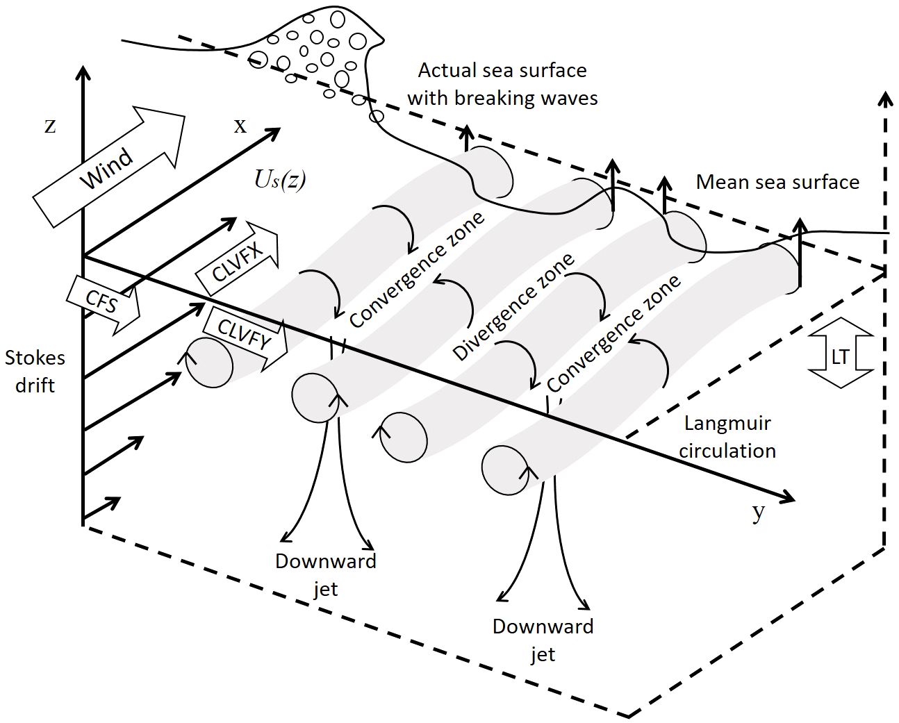
Figure 1 Mixing processes in the upper ocean schematic with vertically sheared Stokes drift and Langmuir cells (grey rolls) created by strong, sustained winds (thick arrow). Stokes drift is a reflection of large-scale wave transportation which contributes directly to the upper ocean mixing. As a result of the interaction between wave-induced Stokes drift and mean-current, downwelling convergence zones and upwelling divergence zones are formed below the surface by the counter-rotating neighboring cells, mostly aligned with the wind. CLVF is an approximation of vortex force acting Eulerian current in the horizontal direction. LT is a continuous source of coherent vertical vorticity.

The sea surface temperature (SST) and ocean current are required by the typhoon/hurricane forecasting model to calculate the air-sea heat and momentum fluxes which are the main contributors to the energy budget of typhoons, thus have a significant impact on the intensity of typhoon. Typhoons/hurricanes cause the upper ocean to react vigorously (Price, 1981; Reichl et al., 2016a, Reichl et al., 2016b), such as the generation of surface waves higher than 20m and the sea surface current > 1m/s, resulting in significant sea surface cooling (Ginis, 2002). The turbulent mixing in the upper ocean boundary layer plays a major role in determining how the SST and current respond to typhoons. When a typhoon passes through a specific location, the large sea surface frictional velocity and surface gravity waves are generated, intensifying the wind-driven mean current shear and Stokes drift. The turbulence caused by vertical shear below the developing surface current significantly deepens the ML (Reichl et al., 2016b). Many studies (Webb and Fox-Kemper, 2011, among others) suggest that SP is the main contributor to the vertical mixing of momentum and temperature/salinity. Accurate knowledge of the kinetic and thermodynamic processes of the ML under strong winds is crucial for marginal waters that are vulnerable to typhoons. By using one-way wave-current coupled model to examine the effects of SP on ocean dynamics in the Bohai Sea during summer, Cao et al. (2019) contend that LT is a common occurrence in the Bohai Sea and has a significant role in modifying the turbulent mixing. Moreover, the role of SP in the upper ocean dynamics under extreme weather such as typhoons deserves further study, since in the operational forecasting, SP terms were not always incorporated in the numerical model.

In this study, we attempt to apply a two-way coupled wave-current model to investigate the upper ocean thermal and dynamic structure responses to SP in typhoon scenarios. Typhoon Matsa (2005) swept over the Bohai Sea is selected as a case. The roles of CSF, CLVF, and LT in modifying the turbulent mixing, thus in changing the thermal and dynamic processes in Bohai Sea, are analyzed through numerical experiments. Parameterizations of the CSF, resolved-scale CLVF, and LT in the dynamic equation are described in Section 2. Section 3 provides information on model coupling and configurations. Section 4 analyzes the numerical results. Conclusions and discussions are presented in Section 5.

2 Parameterization of Stokes production

2.1 Calculation of Stokes drift

Sullivan et al. (2012) suggested that the calculation of Stokes drift should be based on wave spectra, instead of the single-wave assumption or wind-wave equilibrium. After comparative study of several existing computations for Stokes drift, Zhang et al. (2018) also concluded that the Stokes drift might be underestimated when using bulk parameterization. Therefore, here we use directional wave spectra derived by the wave model to calculate Stokes drift. Webb and Fox-Kemper (2011) proposed the leading-order expression for the Stokes drift from an arbitrary spectral shape:

$\begin{array}{ll}{U}_s(z)=\frac{16{\pi }^3}{g}{\displaystyle {\mathrm{\int }}_{\mathrm{0}}^{\mathrm{\infty }}{\displaystyle {\mathrm{\int }}_{-\mathrm{\pi }}^{\mathrm{\pi }}(\cos \theta ,\sin \theta ,0)f^3{S}_{f\theta }(f,\theta )e^{\frac{8{\pi }^2{f}^2}{g}z}d\theta df}}& (1)\end{array}$

In Equation 1 U_s is Stokes drift, S_fθ is the directional-frequency spectral density, θ is wave direction, f is the real wave frequency, and g is the gravitational acceleration.

2.2 Parameterization of CSF and resolved-scale CLVF

According to the schema of McWilliams and Restrepo (1999), we added CSF and CLVF to the horizontal dynamic equations of POMgcs.

$\begin{array}{ll}\frac{\partial UD}{\partial t}+\frac{\partial U^{2}D}{\partial x}+\frac{\partial UVD}{\partial y}+\frac{\partial U\omega }{\partial \sigma }-fVD+ɡ\frac{D^2}{{\rho }_0}{\displaystyle {\mathrm{\int }}_{\mathrm{\sigma }}^{\mathrm{0}}\left[\frac{\partial {\rho }^{\prime }}{\partial x}-\frac{{\sigma }^{\prime }}{D}\frac{\partial D}{\partial x}\frac{\partial {\rho }^{\prime }}{\partial {\sigma }^{\prime }}\right]d{\sigma }^{\prime }+ɡD\frac{\partial \eta }{\partial x}=\frac{\partial }{\partial \sigma }\left[\frac{K_M}{D}\frac{\partial U}{\partial \sigma }\right]+F_x+CSFX+CLVFX}& (2)\end{array}$

$\begin{array}{ll}\frac{\partial VD}{\partial t}+\frac{\partial UVD}{\partial x}+\frac{\partial V^{2}D}{\partial y}+\frac{\partial V\omega }{\partial \sigma }+fUD+ɡ\frac{D^2}{{\rho }_0}{\displaystyle {\mathrm{\int }}_k^0\left[\frac{\partial {\rho }^{\prime }}{\partial y}-\frac{{\sigma }^{\prime }}{D}\frac{\partial D}{\partial y}\frac{\partial {\rho }^{\prime }}{\partial {\sigma }^{\prime }}\right]d{\sigma }^{\prime }+ɡD\frac{\partial \eta }{\partial y}=\frac{\partial }{\partial k}\left[\frac{K_M}{D}\frac{\partial V}{\partial \sigma }\right]+F_y+CSFY+CLVFY}& (3)\end{array}$

where

$\begin{array}{ll}\text{CSFX}=f{V}_{s}D& (4)\end{array}$

$\begin{array}{ll}\text{CSFY}=-f{U}_{s}D& (5)\end{array}$

$\begin{array}{ll}\text{CLVFX}=V_s\left[D\left(\frac{\partial V}{\partial x}-\frac{\partial U}{\partial y}\right)-{\sigma }^{\prime }\frac{\partial D}{\partial x}\frac{\partial V}{\partial \sigma }+{\sigma }^{\prime }\frac{\partial D}{\partial y}\frac{\partial U}{\partial \sigma }\right]& (6)\end{array}$

$\begin{array}{ll}\text{CLVFY}=-U_s\left[D\left(\frac{\partial V}{\partial x}-\frac{\partial U}{\partial y}\right)-{\sigma }^{\prime }\frac{\partial D}{\partial x}\frac{\partial V}{\partial \sigma }+{\sigma }^{\prime }\frac{\partial D}{\partial y}\frac{\partial U}{\partial \sigma }\right]& (7)\end{array}$

In the Equation 2–7, (x, y) are the horizontal coordinates, (U, V) and (U_s, V_s) are eastern-western and northern-southern components of Eulerian mean current and Stokes drift, respectively, CSFX and CSFY are the horizontal components of CSF, and CLVFX and CLVFY are the horizontal components of resolved-scale CLVF.

In addition to vortex force, wave radiation stress is also considered as a mechanism of wave-current interaction. In comparing the effects of the two mechanisms, Moghimi et al. (2013) discovered that vortex force and radiation stress formulations typically produced comparable outcomes. According to Lane et al. (2007), radiation stress may ignore the low-order effect of waves and vortex force is the dominant effect of wave-current interaction. Thus in this study, we merely consider the vortex force.

2.3 Parameterization of LT

It is confirmed that the modification of turbulence parameterization scheme based on Mellor Yamada 2.5 turbulence closure submodel (Mellor and Yamada, 1982, hereinafter MY-2.5) can reveal the wave-induced turbulent mixing. To better simulate the turbulent mixing, a second-moment turbulent closure model of LT, (Harcourt, 2015, hereinafter H15), is used in the present study. H15 changes the corresponding effect of the stability function on Stokes shear, so that the CLVF is directly included in the turbulence closure model. The revised turbulence closure equation can be written as follows:

$\begin{array}{ll}\begin{array}{l}\frac{\mathit{\partial }{q}^{2}D}{\mathit{\partial }t}+\frac{\mathit{\partial }U{q}^{2}D}{\mathit{\partial }x}+\frac{\mathit{\partial }V{q}^{2}D}{\mathit{\partial }y}+\frac{\mathit{\partial }\omega q^2}{\mathit{\partial }\sigma }-\frac{\mathit{\partial }}{\mathit{\partial }\sigma }\left[\frac{K_q}{D}\frac{\mathit{\partial }{q}^2}{\mathit{\partial }\sigma }\right]\\ =-\frac{2}{D}\overline{u\omega }\left(\frac{\mathit{\partial }U}{\mathit{\partial }\sigma }+\frac{\mathit{\partial }{U}_s}{\mathit{\partial }\sigma }\right)-\frac{2}{D}\overline{v\omega }\left(\frac{\mathit{\partial }V}{\mathit{\partial }\sigma }+\frac{\mathit{\partial }{V}_s}{\mathit{\partial }\sigma }\right)+\frac{2g}{{\rho }_0}{K}_H\frac{\mathit{\partial }\tilde{\rho }}{\mathit{\partial }\sigma }-2\frac{D{q}^3}{B_{1}l}+F_q\end{array}& (8)\end{array}$

$\begin{array}{ll}\begin{array}{l}\frac{\mathit{\partial }{q}^{2}lD}{\mathit{\partial }t}+\frac{\mathit{\partial }U{q}^{2}lD}{\mathit{\partial }x}+\frac{\mathit{\partial }V{q}^{2}lD}{\mathit{\partial }y}+\frac{\mathit{\partial }\omega q^{2}l}{\mathit{\partial }\sigma }-\frac{\mathit{\partial }}{\mathit{\partial }\sigma }\left[\frac{K_q}{D}\frac{\mathit{\partial }{q}^{2}l}{\mathit{\partial }\sigma }\right]\\ =E_1{E}_{3}l\frac{ɡ}{{\rho }_0}{K}_H\frac{\mathit{\partial }\tilde{\rho }}{\mathit{\partial }\sigma }+\frac{E_{1}l}{D}\left(-\overline{u\omega }\frac{\mathit{\partial }U}{\mathit{\partial }\sigma }-\overline{v\omega }\frac{\mathit{\partial }V}{\mathit{\partial }\sigma }\right)+\frac{E_{6}l}{D}\left(-\overline{u\omega }\frac{\mathit{\partial }{U}_s}{\mathit{\partial }\sigma }-\overline{v\omega }\frac{\mathit{\partial }{V}_s}{\mathit{\partial }\sigma }\right)-\frac{D{q}^3}{B_1}\stackrel{\sim }{W}+F_l\end{array}& (9)\end{array}$

where

$\begin{array}{ll}\overline{u\omega }=-\left(K_M\frac{\partial U}{\partial \sigma }+K_{MS}\frac{\partial U_s}{\partial \sigma }\right)& (10)\end{array}$

$\begin{array}{ll}\overline{v\omega }=\left(K_M\frac{\partial V}{\partial \sigma }+K_{MS}\frac{\partial V_s}{\partial \sigma }\right)& (11)\end{array}$

$\begin{array}{ll}{K}_{MS}=ql{S}_{MS}& (12)\end{array}$

$\begin{array}{ll}{S}_{MS}=\frac{A_1(1-f_z^s)(1-6A_1/B_1)}{1-9A_1{A}_2{G}_H-9A_1^2(1-f_z^s)l^2{q}^{-2}{D}^{-2}\frac{\partial U}{\partial \sigma }\frac{\partial U_s}{\partial \sigma }}& (13)\end{array}$

In Equation 8–13, $\overline{u\omega }$ and $\overline{v\omega }$ are the components of the vertical turbulent fluxes. According to Kantha and Clayson (2004), q is a turbulence velocity scale, l is a turbulence length scale, D is the water depth. E₁ = E₃ = 1.8, and B₁ = 16.6 are recommended by MY-2.5. E₆ is an LT-related constant, here we choose E₆ = 4E₁. K_MS denotes the new vertical mixing coefficient. S_MS is stability function from H15, A₁ and A₂ are model constants, G_H=-l²q^-2N², N is buoyancy frequency, and $f_z^s$ is the surface-proximity function.

3 Study area and numerical settings

The Bohai Sea, located on the west bank of the Pacific Ocean, is a semi-closed marginal sea in China that may be attacked by typhoons in summer and autumn. In the event of a typhoon, the coastal cities in Bohai Rim Economic Circle, Tianjin, Dalian, and Qinhuangdao may suffer from serious economic loss. It is desirable to build a more accurate operational ocean forecasting and disaster mitigation model with the improved physical mechanism, for example, with the numerical consideration of the effects of SP on the Bohai ocean dynamics in typhoon scenario.

3.1 Wave model configuration

The Simulating Waves Nearshore model (SWAN) that includes processes of wind-wave generation, wave breaking, bottom dissipation, and nonlinear wave-wave interactions, is hired as a wave model to obtain wave parameters and wave spectra (Booij et al., 1999). The input wind field of SWAN is the European Centre for Medium-Range Weather Forecasts (ECMWF) ERA-Interim reanalysis winds, with the input time interval of 6h and a spatial resolution of 0.125°. The wave spectrum was discretized by 32 logarithmically spaced frequencies (with a minimum frequency of 0.05Hz) and 36 evenly spaced directions (with an interval of 10°). The time step is set at 200s, consistent with the internal-mode time step used in the circulation model. The output interval is 6h which is equal to the input interval for the forcing of the circulation model.

The simulation domain covers [37.083°N - 41.033°N, 117.52°E - 122.47°E] (Figure 2) with a horizontal resolution of 0.05°, resulting in grids of 80×100. This setup was carefully chosen to strike a balance between computational efficiency and model accuracy, taking into account the available resolution of bottom topographic data in Bohai Sea. ETOPO2 Global 2’ Elevations dataset is used for bottom topography. The feasibility of such grid configuration had been verified by Cao et al. (2019) and Wang and Deng (2022). The major geographic locations inside the Bohai Sea are: the Liaodong Bay to the north, the Laizhou Bay to the south, the Bohai Bay to the west, the Central Sea Area in the middle, and the Bohai Strait to the east which are connecting the Yellow Sea and are also marked in the right panel of Figure 2.

Figure 2

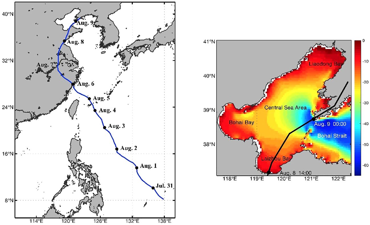
Figure 2 Left: The track of Typhoon Matsa (2005) from 30th July 2005 to 9th Aug 2005 from Zhejiang Provincial Water Resources Department (data source: http://typhoon.zjwater.gov.cn/default.aspx.). Right: Simulation domain of Bohai Sea with the color shading as the water depth (m) and with the major geographic locations names marked. Black line in the right panel represents the track of Typhoon Matsa from 8th Aug to 9th Aug 2005 that directly affected the Bohai Sea.

3.2 Ocean current model configuration

Princeton Ocean Model with generalized sigma-coordinate system (POMgcs, Ezer and Mellor, 2004), a free surface and 3D coastal circulation model, is used to simulate the circulation in the Bohai Sea. The MY-2.5 turbulence closure scheme is included in POMgcs to parameterize the vertical turbulent mixing. Since the majority of Bohai Sea’s water depth is less than 60m, and the ML is where SP has the most influence, the vertical stratification is set at 6 layers, namely 0m, 5m, 15m, 25m, 35m, and 65m. The time step of the internal-mode of POMgcs is set as 200s, and that of the external-mode is set as 0.33s. The initial fields of temperature, salinity, water level, and current velocity are obtained from China Ocean ReAnalysis (CORA), a reanalysis dataset for China’s coastal waters and adjacent seas. They are then interpolated into the computational grid of the model. The model’s domain, bottom topography, and horizontal resolution are the same as those of the wave model specified in section 3.1.

Winds and thermal fluxes are serving as the dynamic driving force of POMgcs. The input wind field of POMgcs is the same as that of wave model SWAN. Nearest neighbor interpolation is applied to reach the model resolution of 0.05°×0.05°, which is adequate to resolve the main dynamic and thermodynamic processes under typhoons. The surface heat fluxes, including long-wave radiation, short-wave radiation, latent heat flux, and sensible heat flux, with a spatial resolution of 1.875°×1.875°, are from the US National Centers for Environmental Prediction (NCEP). To better simulate the vertical structure of temperature in the Summer Bohai Sea, four main tidal components of M2, S2, K1, and O1 are imposed on the open boundary condition of the model. Their feasibility had been well verified by Zhao et al. (2019) and Cao et al. (2019).

3.3 Two-way coupling scheme and experiment setup

POMgcs and SWAN are fully coupled through the model-coupling toolkit (MCT) in two-way data exchange (Figure 3) with an exchange frequency of 1800s. The input to the SWAN is the output of real-time current and sea surface height from POMgcs. The CSF, CLVF, and LT are calculated using wave spectrum and parameters output from the SWAN, then fed to POMgcs. Comparing to the one-way coupling model (without the feedbacks from POMgcs to SWAN), we are expecting that this coupling would allow for a more comprehensive examination of the intricate interplay between waves and currents, enabling a more accurate representation of the dynamic processes occurring in the Bohai Sea under typhoon conditions.

Figure 3

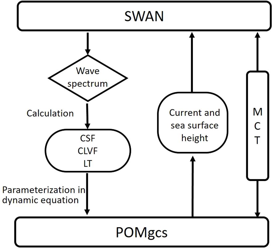
Figure 3 Schematic of POMgcs-SWAN two-way coupling.

The integration time of the numerical experiment is half a year, from 1^st January to 31^st July 2005, in order to obtain a stable current field. The vertical stratification of the Bohai Sea in summer is stronger and more stable, and the influence of convective mixing on the mixing layer is relatively weak, which makes the influence of SP more significant. Four diagnostic experiments are designed in this study (Table 1): (1) the control run (WAVE-NONE), in which the wave effects are not considered, serves as the benchmark to measure the effects of CSF, CLVF, and LT on ocean dynamics, (2) adding both CSF and CLVF (WAVE-CSVF) in the horizontal momentum equations, (3) only introducing LT parameterization (WAVE-LT), and (4) including CSF, CLVF, and LT parameterization (WAVE-ALL).

Table 1

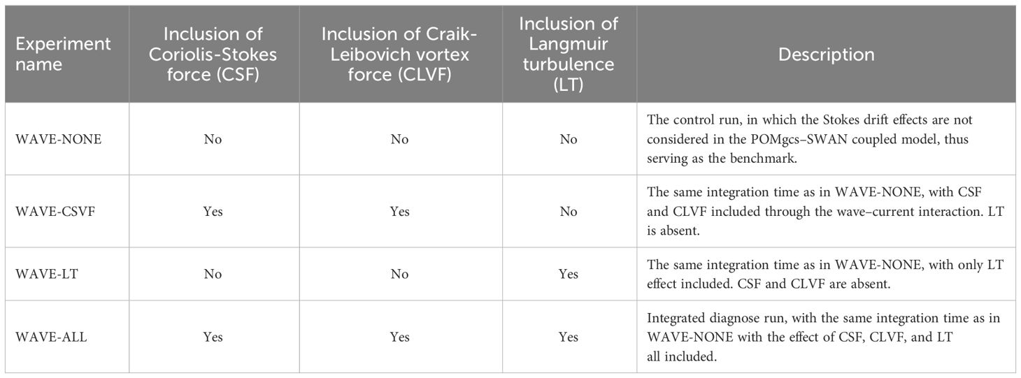
Table 1 Experiment setup.

4 The modeling results

Typhoon Matsa, which swept over the Bohai Sea in 2005, was selected as the case study. Initiated at 2000 UTC+8, 31^st July 2005 in the ocean east of Philippine at [134°E, 11.7°N], Typhoon Matsa developed into a tropical storm on 2^nd August and then strengthened to a mature typhoon by 5^th August 2005 with steady winds of around 150 km/h. Moving northwest, Masta made landfall at Yuhuan County Zhejiang Province at 0340 UTC+8, 6^th August 2005 with a peak intensity and maximum sustained wind (MSW) of 45m/s (Song, 2012). The weakening tropical cyclone then passed through Zhejiang, Anhui, Jiangsu, and Shandong Provinces successively before the center of Matsa entered the Bohai Sea from Lazhou Bay around 1400 UTC+8, on 8^th August, with a maximum sustained wind speed up to 18m/s and a central mean-sea-level pressure of 995 hpa. Matsa was downgraded to a temperate cyclone at 0500 UTC+8, on 9^th August in the central area of Bohai Sea, then it made a second landfall at Dalian, Liaoning Province two hours later.

The Bohai Sea was primarily affected by Typhoon Masta between 8^th and 9^th August 2005. Three stages are set in the present study with 0000UTC on 7^th August representing pre-typhoon condition, 0000UTC on 8^th and 9^th August standing for the typhoon stage, and 0000UTC 10^th August as the after-typhoon stage. LT on the ocean dynamic process of Bohai Sea under typhoon condition is then studied. This allows for the analysis of the upper ocean response of the Bohai Sea to Typhoon Masta. ECMWF ERA-Interim reanalysis wind field are hired to study the wind speed distribution over Bohai Sea during the four days mentioned above.

On 7^th Aug, low winds ranging between 4 and 8 m/s were observed, which are the typical of what the Bohai Sea experiences during the summer. The wind speed in the entire sea area elevated dramatically on 8^th and 9^th August, when Typhoon Masta was in the Bohai Sea, reaching a maximum wind speed of ~20m/s on 8^th August. The typhoon center gradually moved from the Bohai Strait to the northeast, then reached the central sea area, with a rapid weakening of typhoon intensity. The maximum wind speed on 9^th August decreased to 12 m/s. Then, the wind speed after typhoon (10^th August) dropped quickly, with slightly higher winds than the pre-typhoon stage. However, Typhoon Masta did alter the wind direction over the Bohai Sea on 10^th August, which was opposite to that on 7^th August.

The harshness of the sea is typically measured by the significant wave height (H_s), one of the most important wave parameters for characterizing wave energy. Table 2 shows the single-point H_s comparison of the model simulation with the in-situ observations at the tide gauge stations of Laohutan¹ from 7 to 10 August 2005. The RMSE (Root Mean Square Error) of less than 0.01, and the CC (Correlation Coefficient) exceed 90%, indicating that the model is relatively reliable in simulating the significant wave height. A typhoon can easily generate large gravity waves thus leading to a significant increase in H_s. The distribution of H_s output by SWAN shows relatively good agreement with the wind field on 7^th August, when the wind speed was low or moderate across the entire Bohai Sea, and on 8^th August when Typhoon Matsa first stepped into the study region with strong power and high speed (Figures 4A, B). During these stages of pre-typhoon and during-typhoon, the directions of Stokes drift were basically as same as that of wind (Figures 4E, F), suggesting a generally positive correlation between them. When the Matsa exerted its influence on the Bohai Sea as a complete cyclone on 9^th August, the typhoon center (39°N, 120°45′E) in the central sea area was inconsistent with the counter-clockwise drift center (38°30′N, 120°E) formed by Stokes drift (Figure 4G), and the direction deviation in wind and Stokes drift was large within this area. It is interesting to find that the area with large H_s(>0.4m) was located east to the Bohai Strait adjacent to (38°N, 120°45′E) (Figure 4C). In after-typhoon stage of 10^th August, the H_s in the Bohai Bay and west Liaozhou Bay dropped to<0.2m while remaining high in the Bohai Strait (Figure 4D). A relatively large Stokes drift of 0.01~0.015 showed up in the northeast Laizhou Bay and southwest Bohai Strait, with direction aligned with that of the wind field. The maximum Stokes drift of the study region appeared in the Yellow Sea near the southern tip of Liaodong Peninsula which agrees well with the largest H_s (Figure 4H).

Table 2

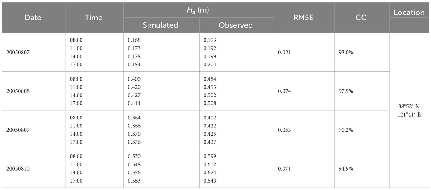
Table 2 Model validation with in-situ observations.

Figure 4

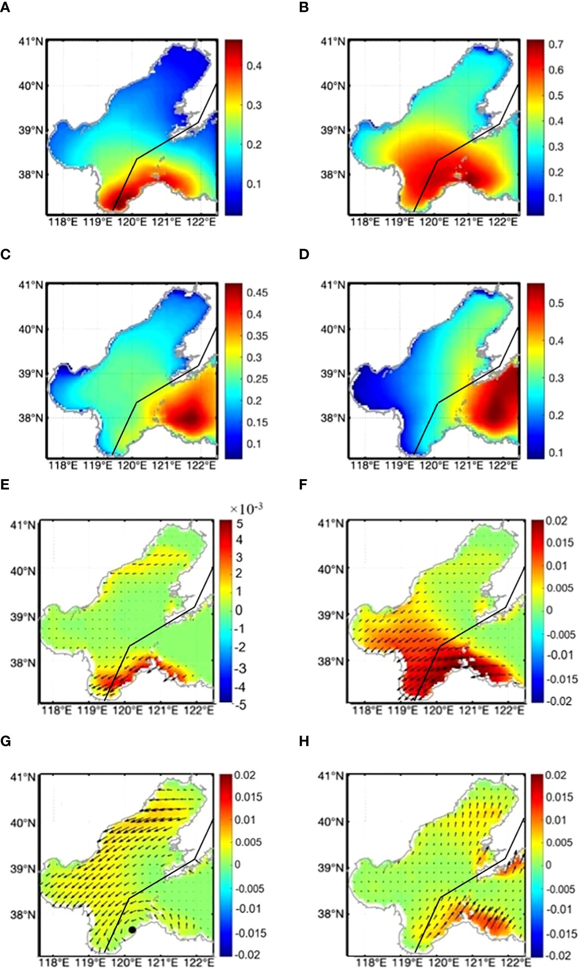
Figure 4 POMgcs simulated horizontal distribution of significant wave height (m) without coupling at 0000 UTC on (A) 7^th, (B) 8^th, (C) 9^th, and (D) 10^th August 2005. Horizontal distribution of simulated Stokes drift direction and speed (10^-3 m/s) on (E) 7^th, (F) 8^th, (G) 9^th, and (H) 10^th of August 2005. Black line represents the track of Typhoon Matsa from 8th to 9th Aug 2005. Black dot in (G) represents the center of counter-clock-wise Stokes drift.

Through the above analysis, we were able to observe the numerical response of wave field to wind, where high wind causes big H_s, as well as the complicated variation of Stokes drift due to the wave-current interactions under severe weather. Stokes drift responds to normal wind relatively quickly and simply, while there seems to be a temporal lag in a typhoon scenario. The magnitude and direction of Stokes drift are also influenced by the elevated current in high winds, thus not aligned with the winds.

4.1 Temperature

To quantitatively study the influence of different SP terms on sea temperature, the deviations between different diagnostic experiments and control run WAVE-NONE were calculated. The sea surface temperature (SST) simulated by WAVE-ALL was found to be lower than that of WAVE-NONE on 7^th August 2005, prior to the arrival of Typhoon Masta in the majority of the Bohai Sea. In particular, the temperature decreased evidently by about 0.3°C in the south of Liaodong Bay, the east of Bohai Bay, and the sea area near Miaodao islands. Under normal weather conditions, the Bohai Sea has a clear and stable vertical temperature stratification. However, the presence of SP in the numerical model slightly reduced the temperature at sea surface and a few meters below, while slightly increased the temperature of the deeper layer (such as the layers of 15m and 25m). In general, the overall vertical temperature change was insignificant, and the temperature stratification structure essentially remained unchanging, suggesting a minimal effect of SP on the vertical temperature profile in the Bohai Sea. When comparing our current two-way coupling approach with the one-way coupling employed in Cao et al. (2019), which demonstrated a reduction in sea surface temperature (SST) by less than 0.4°C across most of the Bohai Sea region under normal conditions, we observe an increase in the maximum SST deviation to 0.5356°C in our (WAVE-ALL)-(WAVE-NONE). Although the simulations were not conducted on the exact same day, this discrepancy partly underscores the influence of wave-current feedback on local thermodynamics. Given the absence of in-situ observation during our simulation experiments, it is premature to definitively assert the superiority of either approach. However, it is evident that the two-way coupling incorporates a more comprehensive physical mechanism, rendering it theoretically advantageous.

When Typhoon Masta entering the Bohai Sea (8^th August), the SST decreased rapidly, and the SP aggravated the “cold absorption” of the sea water, resulting in a maximum decline of 0.4°C in the SST. Reichl et al. (2016a) discovered that when the SST drops by 0.5°C, the total air sea heat flux falls by at least 10%, suggesting this SST cooling caused by SP cannot be ignored in the ML parameterization under severe weather. By comparing with the pre-typhoon stage, it can be seen that, owing to the enhancement of sea surface wind and the deterioration of sea state by typhoon, the SP effect intensified, resulting in a significant increase in both the cooling magnitude and range of the SST (Figure 5B).

Figure 5

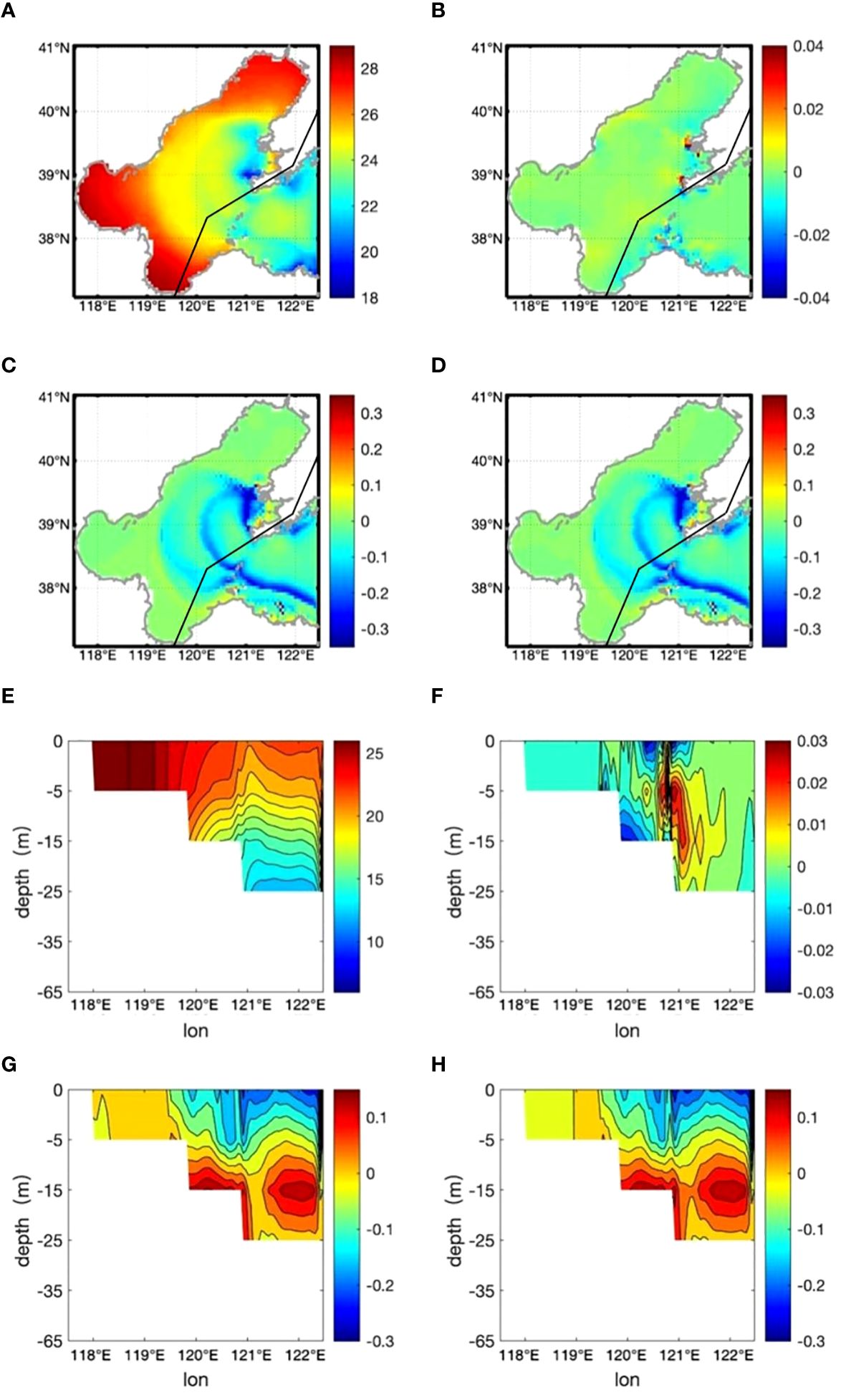
Figure 5 Horizontal distribution of (A) SST from WAVE-NONE, and SST difference between (B) (WAVE-CSVF) - (WAVE-NONE), (C) (WAVE-LT) - (WAVE-NONE), and (D) (WAVE-ALL) - (WAVE-NONE) at 0000UTC on 8^th August 2005 (°C). Black line represents the track of Typhoon Matsa from 8th to 9th Aug 2005.Vertical temperature profile along the widest section in Bohai Sea 38.333°N from (E) WAVE-NONE, and the temperature differences between (F) (WAVE-CSVF) - (WAVE-NONE), (G) (WAVE-LT) - (WAVE-NONE), and (H) (WAVE-ALL) - (WAVE-NONE) at 0000UTC on 9^th August 2005 (°C).

Masta did not induce a significant change in the vertical temperature structure when it initially entered the Bohai Sea. However, after one day’s working, the temperature difference of the whole central sea area and the Bohai Strait became evident, with the maximum temperature change exceeding 0.41°C. This occurred because these areas have a deeper water depth, which allows the SP to continue bringing colder water up to the surface. Even though the intensity of Typhoon Masta on 9^th August was substantially lower than it was one day before, the heat exchange between the upper and lower sea water caused by SP was still in progress, causing a lag in temperature change. Vertically, the temperature stratification gradually weakened, and the upper and lower layers became increasingly mixed (Figure 5G). The SP makes the cooling of the sea surface more obvious. The difference of the vertical temperature profile is greater (comparing Figures 5E, G), with a maximum decrease of 0.54 °C. It is anticipated that if the typhoon persists for longer, the SP will cause more intense vertical heat exchange. The similar pattern of Figures 5G, H implies that the effect of LT in elevating the turbulence mixing is stronger than that of CSF and CLVF.

4.2 The ocean currents

Along with the increased wind speed caused by Masta starting from 8^th August, the surface current speed increased accordingly, especially in the marginal areas of east Bohai Bay and the northwest Laizhou Bay (Figure 6A). The Liaodong Bay in northeast Bohai Sea had not been affected by the typhoon, thus the surface currents there for four experiments remained close to the pattern on 7^th August. With the consideration of CSF and CLVF in WAVE-CSFV case (Figure 6B), the maximum current speed increase of 0.018m/s and maximum reduction of 0.013m/s all appeared in the Bohai Strait. From Figure 6C, the maximum change of surface current speed brought by LT under typhoon weather was 0.04m/s, and the maximum speed change area basically coincides with that of the maximum temperature change. The similar pattern of Figures 6C, D suggests that among the SP terms, LT has a greater influence on the vertical mixing intensity and TKE during typhoon.

Figure 6

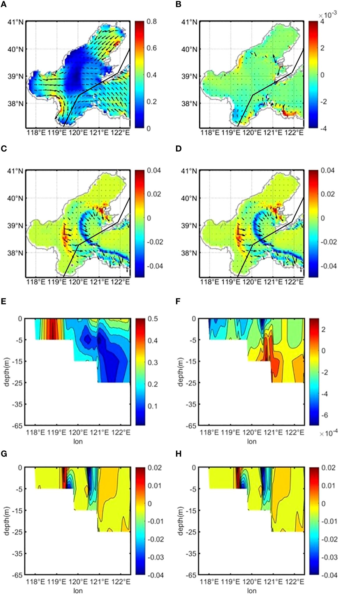
Figure 6 Horizontal distribution of (A) surface current (unit: m/s) of WAVE-NONE, (B) current difference (unit: m/s)between WAVE-NONE and WAVE-CSVF, (C) current difference between WAVE-NONE and WAVE-LT, and (D) current difference between WAVE-NON and WAVE-ALL at 0000UTC on 8^th August 2005. The color shading represents the magnitude of current velocity, and the arrows represent the current direction. Black line represents the track of Typhoon Matsa. The Vertical profile of current velocity along the 38.333°N section at 0000UTC on 8^th August 2005 from (E) WAVE-NONE, and the differences between (F) (WAVE-CSVF) - (WAVE-NONE), (G) (WAVE-LT) - (WAVE-NONE), and (H) (WAVE-ALL) - (WAVE-NONE).

The vertical profiles of current and related changes along the 38.333°N section simulated by four experiments on 8^th August 2005 are shown in Figure 6E to Figure 6H. Numerically, the presence of SP occupied a portion of the energy transmitted to the upper ocean by winds. Typhoon Masta generally made the current distribution in the whole shallow sea become more uniform, and the presence of SP further promoted the decrease of simulated speed throughout the entire water depth. However, because of the short time of typhoon, the intensification of wind force led to a rapid increase in surface current speed, and the kinetic energy transmitted from the atmosphere to the sea was mainly limited to a depth of several meters below the sea surface. In other words, within a short time period, energy transfer to the lower layers was insufficient, resulting in the vertically stratified currents in the central sea area and the Bohai Strait, and there was a significant difference between the surface velocity and the bottom velocity. In certain areas, there is a noticeable change in the direction of the current vectors.

With 24h action of typhoon winds, the increased sea surface current speed agreed well with the areas of high wind speed, while the speed was quite low near the center of the typhoon. The influence of the wind direction can be reflected in the current direction. At the pre-typhoon stage, the current mainly converged from other areas to the Laizhou Bay. On 9^th Aug, the current direction in the Laizhou Bay gradually became parallel to the wind direction, indicating that the wind was the dominant factor affecting the current during the typhoon, rather than the tidal currents. When the typhoon continued to act, the influence of SP on the surface current speed was further enhanced, and the decrease of sea surface speed was most obvious in the northern Laizhou Bay and the Bohai Strait. Vertically, the energy transported by the atmosphere to the ocean has been fully propagated to the whole depth. Because of the shallow water depth, the current velocity at the surface and bottom were almost the same. In the Bohai Bay and the central sea area, the current speed increased significantly because of the consistent wind direction and the circulation direction, while in the Bohai Strait the speed was smaller due to its proximity to the typhoon center and the opposite wind direction to the original circulation. With SP under typhoon conditions, the vertical structure of the current changed noticeably, with the speed decreasing more along the vertical direction.

On 10^th Aug, as Matsa passed, the currents were mostly flowing eastward, from the Liaodong Bay and the Bohai Bay to the Laizhou Bay and the Bohai Strait. In the Bohai Bay and the central sea area, the current speed decreased, while in the Bohai Strait, the speed increased. With the weakening of the sea surface winds, the ocean current started to change from the surface to the bottom, thus forming a temporary current stratification. Comparing the distribution of WAVE-NONE and WAVE-ALL (Figure 7), the consideration of SP promoted the synergetic current change at the upper and lower layers, making the current distribution more uniform in the vertical direction. In other words, the SP weakened the current stratification to a certain extent.

Figure 7

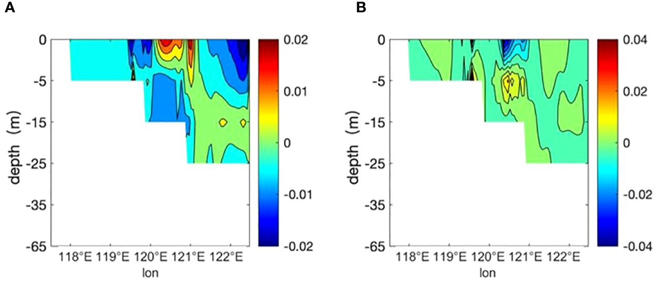
Figure 7 The vertical profile of current velocity differences (unit: m/s) between (WAVE-ALL) - (WAVE-NONE) along the 38.333°N section at 0000UTC on (A) 9^th and (B) 10^th August 2005.

4.3 Turbulent Langmuir number and vertical mixing coefficient

Turbulent Langmuir number (L_a) is an indicator representing the relative influence of wind driven shear and Langmuir turbulence (McWilliams et al., 1997). By using the parameterization proposed by Harcourt and D’Asaro (2008), the nondimensional number $L_a=\sqrt{{(\left|{\rho }_{a }{C}_d\right|\overrightarrow{u_{10}}\overrightarrow{|u_{10}}/\rho |)}^{\raisebox{1ex}{$1$}\!\left/ \!\raisebox{-1ex}{$2$}\right.}{/|\langle U_s\rangle }_{SL}-U_s(z_{ref})|}$, spatial distribution of the Langmuir turbulence is calculated. In the calculation, ρ is the sea water density and ρ_a is the air density, u₁₀ is the 10-m wind speed, C_d is the wind drag coefficient and following the form proposed by Zijlema et al. (2012), 〈U_s〉_SL is the Stokes drift averaged over the surface layer, U_s(z_ref) is the reference Stokes drift, and z_ref represents the mixed layer depth.

The daily-mean L_a values in the Bohai Sea during the whole typhoon event are given in Figure 8. L_a represents the ratio of viscous to inertial forces in the water column, i.e., in negative correlation with sea surface Stokes drift. At pre-typhoon stage, although some high L_a values appeared near the central line in Bohai Strait, most of the Bohai Sea had L_a less than 0.3 (Figure 8A). This is lower than the typical range of 0.35~0.5 reported by Belcher et al. (2012) for the Northern Hemisphere in summertime, indicating the important role of Langmuir turbulence in the Bohai Sea. During the typhoon, strong atmospheric forcing caused a decrease in L_a throughout the Bohai Sea, with the value falling below 0.14 on 9^th Aug (Figure 8C), and below 0.16 on 10^th Aug 2005 (Figure 8D).

Figure 8

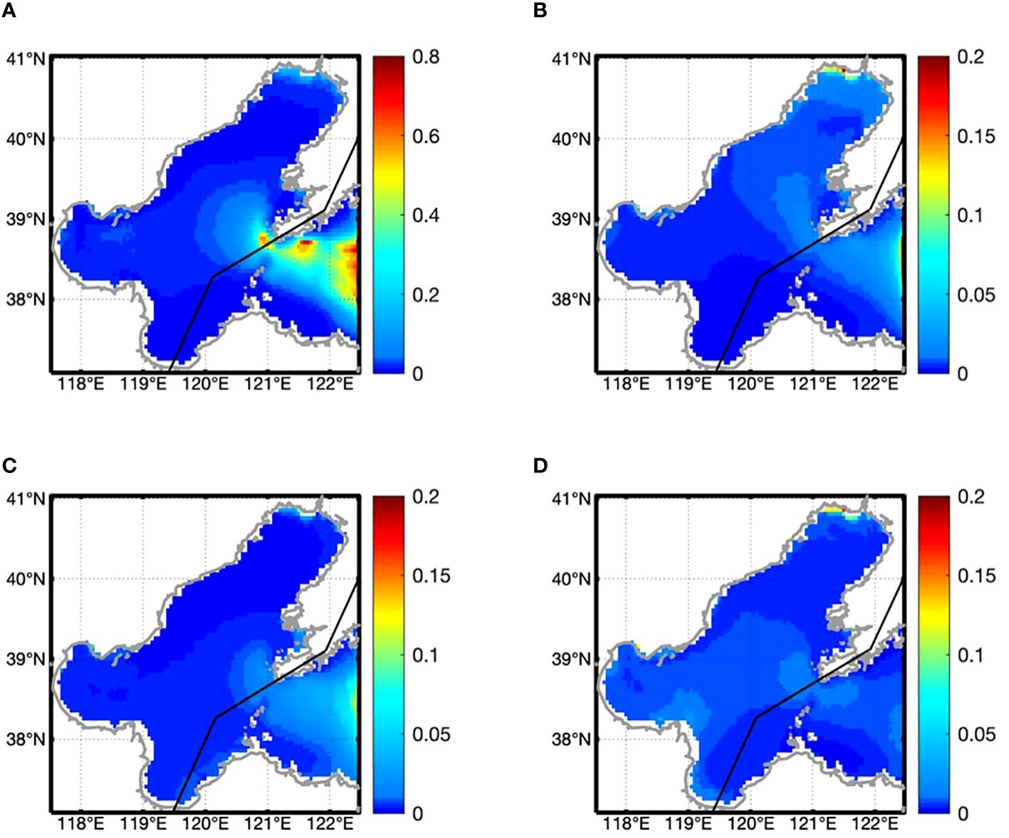
Figure 8 Horizontal distribution of daily mean Langmuir number on (A) 7^th, (B) 8^th, (C) 9^th, and (D) 10^th August 2005. Black line represents the track of Typhoon Matsa.

Wind can directly affect the turbulent mixing of the upper ocean. The distribution of vertical mixing coefficient was positively correlated with the wind field. This study compares the K_M (without LT) and K_MS (with LT) that was calculated by Equation 12 following H15 parameterization for Langmuir circulation.

Under normal weather conditions (represented by 7^th Aug), the vertical mixing coefficient K_MS that includes the SP effect, was greater than the original vertical mixing coefficient K_M at the surface, 5m, and 15m layers. However, the SP did not alter the horizontal structure of the vertical mixing coefficient, thus the vertical profile of K_MS was basically identical to K_M, especially at depths greater than 35m (Figure 9A). This indicates that although Stokes drift decayed exponentially within a few meters below the sea surface, the LT it generated continued to transmit downward and enhanced the turbulent mixing of the entire upper ocean. Under typhoon condition, K_MS was obviously larger than K_M at the upper 25m on 8^th Aug and extended to upper 55m on 9^th Aug (Figures 9B, C). One day after Typhoon Matsa’s passage, K_MS slightly decreased but was still larger than K_M at almost all depths (Figure 9D).

Figure 9

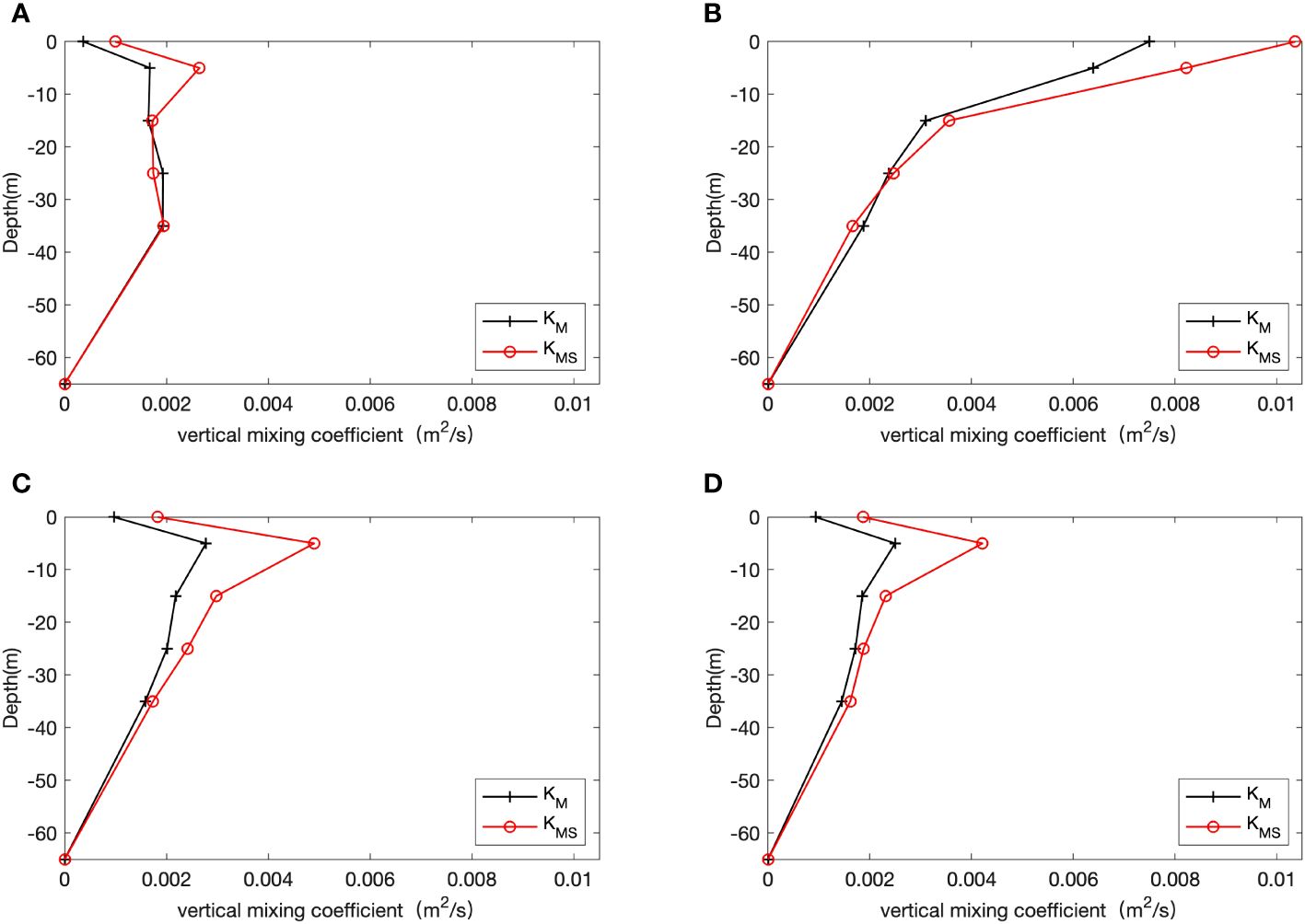
Figure 9 The profile of horizontally averaged vertical mixing coefficients K_M and K_MS (m²/s) simulated at 0000UTC on (A) 7^th, (B) 8^th, (C) 9^th, and (D) 10^th August 2005 in Bohai Sea, where the black line with + represents the profile without wave effect (WAVE-NONE), while the red line with circle shows the situation with CSF, CLVF, and LT (WAVE-ALL).

Through examination of the horizontal distribution of the sea surface mixing coefficient in the Bohai Sea, it is found that the vertical mixing coefficient increased significantly when Typhoon Matsa swept the sea surface with a maximum increase of O(10 m²/s) on 8^th August near the north boundary of Laizhou Bay (~38.2°N). The higher the wind speed, the greater the vertical mixing coefficient. K_MS was larger than K_M with a maximum difference of 0.02 m²/s, suggesting that the wind speed has a greater impact on K_MS when SP is taken into account. On 9^th August, the regions with enlarged mixing coefficient were in the Laizhou Bay and the southern Bohai Strait, both of which experienced strong winds. In the typhoon center and the regions with large difference between Stokes drift direction and wind direction, the vertical mixing coefficient was very small. This agrees with the previous studies (Van Roekel et al., 2012; Zhang et al., 2018) which found that wind wave misalignment can obviously suppress Stokes drift and turbulent mixing caused by shear effect. After the wind speed dropped to be less than 8m/s on 10^th Aug, the mixing coefficient in the Lazhou Bay and Bohai Strati remained at a higher level than that of the pre-typhoon stage. The presence of SP significantly influenced the K_MS, with a maximum difference of 2.8×10^-3m²/s between K_MS and K_M.

4.4 The mixed layer depth (MLD)

The MLD is another important feature for the vertical temperature distribution in typhoon simulations. In this study, MLD is computed based on a constant temperature difference criterion, specifically the 0.5°C temperature difference between the ocean surface and the bottom of ML (Monterey and Levitus, 1997). We first interpolated the simulated sea water temperature layer by layer in horizontal direction, and then calculated the depth of ML by using the above criterion. Figure 10 shows the MLD simulated by the cases of WAVE-NONE, WAVE-CSVF, WAVE-LT, and WAVE-ALL along the 38.333°N section at pre-, during-, and after- Typhoon stages, respectively. Under normal and typhoon weathers, the MLD was basically equivalent to the depth of water in shallow offshore regions, where the whole depth of sea water was well mixed with similar temperature at the sea surface and bottom layer. When the longitude exceeds 119°E, the thickness of the ML decreased rapidly and remained stable within 1m on 7^th Aug 2005 (Figure 10A). This is due to the strong vertical stratification in the summer Bohai Sea, with a large temperature difference between the sea surface and subsurface. Comparing the results of four experiments at the pre-typhoon stage, we found little variation in MLD, which could be ignored from the perspective of the whole Bohai Sea.

Figure 10

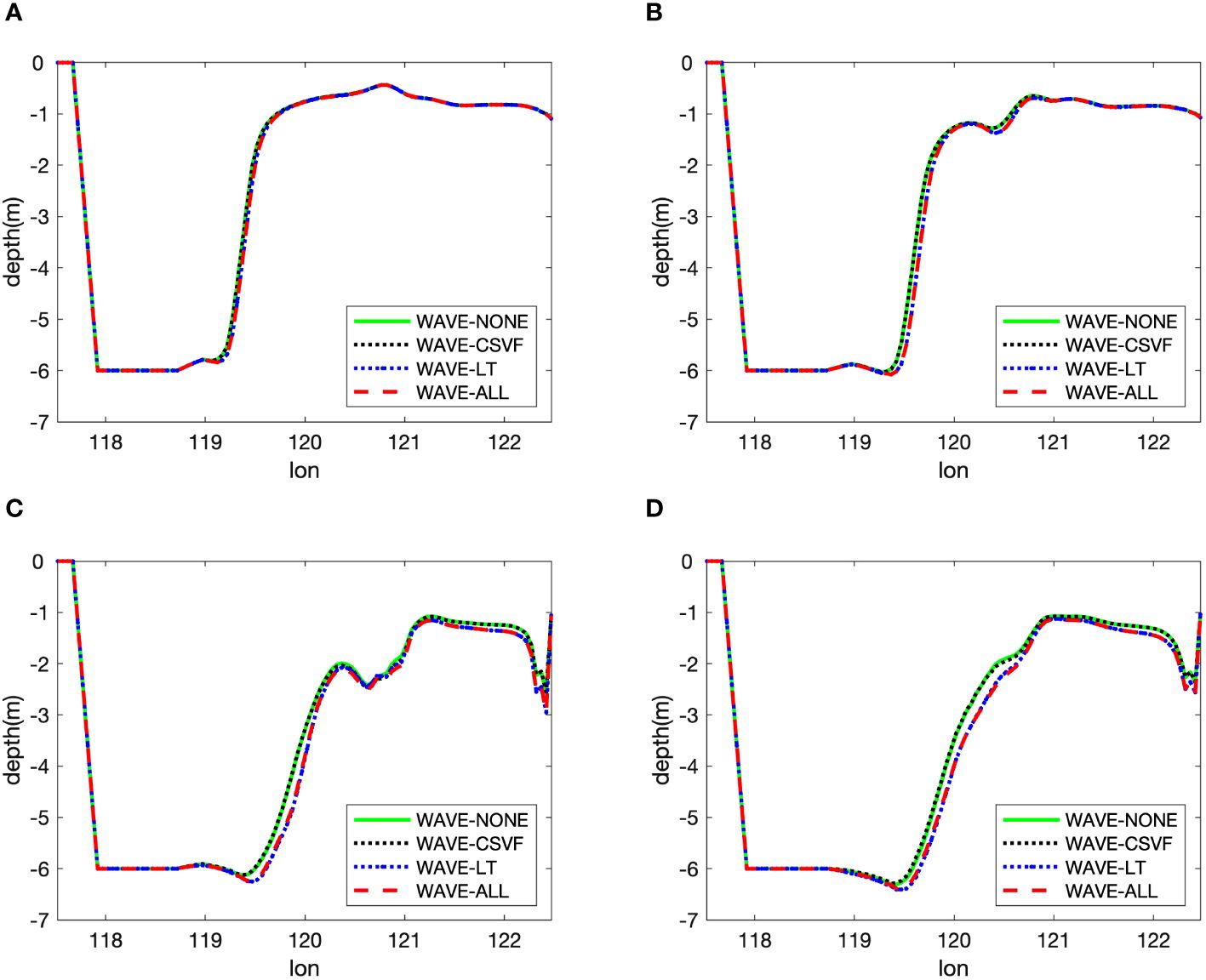
Figure 10 Mixed layer depth (M) along the section 38.333°N in Bohai Sea at 0000UTC on (A) 7^th, (B) 8^th, (C) 9^th, and (D) 10^th August 2005, in which the green solid lines represent coordinate run without consideration of wave, black dots are the simulation with CLVF and CSF, blue dots show the simulation with LT, and the dashed red line are the result of all wave effects.

When Typhoon Matsa entered the Bohai Sea on 8^th Aug, the MLD in the deep sea area began to deepen, especially for [119.5°E-120.7°E] (Figure 10B). The MLD is sensitive to different mixing schemes, with MLD generated by WAVE-ALL and WAVE-LT thicker than those simulated by WAVE-NONE and WAVE-CSVF, indicating that the incorporation of additional SP terms does affect the deepening of the ML. Under the continuous action of typhoon, the MLD in the Bohai Sea was further deepened on 9^th Aug, and the MLD in deep water areas (east of 119°, >20m depth) was all larger than 1m. Only at 120°50′E close to the center of typhoon, the MLD decreased rapidly to about 1.1m (Figure 10C), which is consistent with the results of Reichl et al. (2016b). The largest MLD difference between WAVE-ALL and WAVE-NONE was 0.65m. Compared with temperature section in Figure 5, it can be found that the seawater within the ML was fully mixed and exhibited a uniform vertical temperature distribution. From the results of WAVE-NONE and WAVE-ALL, we can see the continued influence of SP on strengthening of the upper mixing.

Without strong atmospheric forcing at the after-typhoon stage, the MLD gradually returned to smaller value on 10^th Aug. The MLD obtained by WAVE-ALL simulation was deeper than that of WAVE-NONE, with a larger difference of 0.5m around [120°E-120.4°E], and about 0.1~0.2m in other areas. Because of the lag of ocean response to atmospheric force, these changes of MLD induced by SP were of the same magnitude with that on 9^th Aug when typhoon passed by.

5 Conclusion and discussion

This paper studies the influence of the SP on the ocean dynamics and thermal processes of the Bohai Sea during Typhoon Matsa based on fully coupled wave-current model simulations. The 0000UTC of each day from 7^th to 10^th August, 2005 are selected to represent the pre-, during-, and after-typhoon stages, respectively. The main findings include:

(1) Before typhoon arrived in the Bohai Sea, on 7^th August 2005, the Stokes drift caused slight decrease of the SST and an increase in temperature at deeper layers, but the temperature stratification structure generally remained unchanging. The SP terms had little effect on the MLD and sea surface current speed in the Bohai Sea. By analyzing the vertical mixing coefficient K_M and K_MS, it can be found that the mixing coefficient is positively correlated with the wind speed, and the SP strengthens the vertical mixing intensity.

(2) On 8^th August 2005 when Typhoon Matsa was sweeping over the Bohai Sea, the Stokes drift intensified the turbulent mixing in the upper ocean, resulting in a significant decrease in SST and current speed, and a thicker ML. However, due to the short action time of typhoon in the Bohai Sea, the vertical temperature structure was not changed dramatically, and the kinetic energy transmitted from the atmosphere to the sea was mainly limited to the surface layer. The current starts to be stratified in the vertical direction with relatively large speed difference between the surface and the bottom. From the distribution of vertical mixing coefficient, it can be seen that wind speed has a higher impact on K_MS when taking the SP into account.

(3) On 9^th August 2005, one day after typhoon influencing the Bohai Sea, the continuous effect of SP brought deeper colder water to the surface, leading to the significant surface water cooling and the gradually weakened temperature stratification. The vertical temperature structure was almost changed, and the MLD decreased rapidly to about 1.1m. The presence of SP makes the speed decrease more in the vertical direction, while the vertical structure of current tends to be more uniform. The magnitude of K_MS is mainly controlled by the wind speed and the angle between wind direction and Stokes drift direction, and the misaligned wind and wave fields can obviously suppress the turbulent mixing caused by SP.

(4) After the passage of Typhoon on 10^th August 2005, the SST in the Bohai Strait and the central sea area decreased in the SP involved parameterization. The magnitude and range of the temperature decrease were similar to those on 9^th August. This suggests that the SP not only affects the SST on the synoptic time scale, but also has a longer time scale influence, which is correlated with the total heat budget on the monthly and seasonal scales. Comparing the vertical temperature simulated by WAVE-ALL and WAVE-NONE, it can be found that with SP the temperature difference of -0.01°C largely occurred in ML, while from the bottom of ML downward to the seafloor only a small positive value scattered. Actually, from the simulation of successive days, it is suggested that the warming trend in the ML is slow, and the depth of the ML changes slowly, indicating the response lag of seawater temperature to the SP. The current gradually returned to the normal wind condition, with the SP terms promoting the coordinated change of upper- and lower-layer currents, thus making the current velocity distribution more uniform in the vertical direction. Although the wind speed in most areas of the Bohai Sea dropped to<8m/s, the vertical mixing coefficient maintained a large value in some areas.

The above findings are consistent with the previous studies that the improvement of surface gravity waves parameterizations for mixing is essential to depict the upper ocean dynamic and thermodynamic structure. In the typhoon scenario, the intensified wave-induced mixing led to the elevated vertical mixing coefficient, deepened MLD, and sea surface cooling as expected. High wave regions tend also to be regions of high Stokes drift, however, in some areas it is not the case, since stokes drift is also correlated with other characteristics of surface gravity waves, such as wave speed. Our statistical analysis reveals marginal improvements in results with the two-way coupling over one-way coupling of POMgcs and SWAN, as it also integrates the feedback of currents on waves, leading to localized adjustments in simulation outcomes without inducing significant changes. For instance, in our pre-typhoon experiment, the average difference between (WAVE-ALL) and (WAVE-NONE) current speed is approximately -0.0013 m/s. This finding aligns closely with Cao et al.’s (2019) one-way coupling simulation, indicating that velocities derived from (WAVE-NONE) tend to be larger than those from (WAVE-ALL). In the present study, we use limited buoy observation data to validate and illustrate the simulation’s efficacy in representing H_s, further reinforcing the credibility of our two-way coupling model. However, due to article length constraints and limited field observations, we refrain from presenting a detailed comparative analysis between two-way and one-way coupling simulations in this paper. Our focus lies on utilizing modeling tools to delve into Stokes drift and Langmuir turbulence effects. Nevertheless, it’s crucial to underscore that two-way coupling offers a more comprehensive physical mechanism, theoretically enhancing the fidelity of numerical simulations in shallow marginal seas.

It is also worth noting that the present study focuses on the impact of three SP terms on upper ocean dynamics under typhoon scenario based on a two-way coupled wave-current model, rather than providing an exhaustive analysis of specific regional characteristics. This methodological framework can be adapted and applied to various other coastal sea areas, enabling researchers to explore and understand the dynamics of Stokes drift in diverse marine environments. In the future, the numerical study of the role of SP in normal weather conditions and typhoon scenario in a fully coupled system of atmospheric-wave-current model would be desirable. As mentioned in Section 1, this study does not discuss the effect of wave-breaking, which has a considerable effect on the near-surface distributions of current, temperature, and salinity. Also, the integration of wave-breaking together with SP in the coupled ocean model remains a direction to be explored, as under high-wind conditions, the wave-breaking injects TKE to near-surface depths and the sea spay it induced can impact the exchange processes of momentum and heat through air-sea interface thus affecting ocean circulation modeling.

The impact of SST on hurricane intensity forecasts is a good example that emphasizes its importance in the air-sea interaction. A decrease of SST due to entrainment of the cooler waters from the thermocline in the ML under hurricane wind forcing produces a significant change in storm intensity.

Data availability statement

The original contributions presented in the study are included in the article/supplementary material. Further inquiries can be directed to the corresponding authors.

Author contributions

TY: Conceptualization, Funding acquisition, Validation, Writing – original draft, Writing – review & editing. ZD: Conceptualization, Formal Analysis, Funding acquisition, Investigation, Methodology, Resources, Validation, Writing – review & editing, Writing – original draft. CZ: Formal Analysis, Validation, Visualization, Writing – review & editing. AA: Formal Analysis, Validation, Writing – review & editing.

Funding

The author(s) declare that financial support was received for the research, authorship, and/or publication of this article. This research was supported by the National Key Research and Development Program under contract No. 2022YFC3105002; the National Natural Science Foundation under contract No. 42176020; and the Chinese Academy of Engineering Advisory Project under contract No. 2022-XBZD-11.

Conflict of interest

The authors declare that the research was conducted in the absence of any commercial or financial relationships that could be construed as a potential conflict of interest.

Publisher’s note

All claims expressed in this article are solely those of the authors and do not necessarily represent those of their affiliated organizations, or those of the publisher, the editors and the reviewers. Any product that may be evaluated in this article, or claim that may be made by its manufacturer, is not guaranteed or endorsed by the publisher.

Footnotes

1. ^ Oceanographic station observations are available at NMDIS, http://www.nmdis.org.cn.

References

Belcher S., Grant A., Hanley K. (2012). A global perspective on Langmuir turbulence in the ocean surface boundary layer. Geophys. Res. Lett. 39, L18605. doi: 10.1029/2012GL052932

CrossRef Full Text | Google Scholar

Booij N., Ris R. C., Holthuijsen L. H. (1999). A third-generation wave model for coastal regions - 1. Model description and validation. J. Geophysical Research-Oceans 104, 7649–7666. doi: 10.1029/98JC02622

CrossRef Full Text | Google Scholar

Cao Y., Deng Z., Wang C. (2019). Impacts of surface gravity waves on summer ocean dynamics in Bohai Sea. Estuarine Coast. Shelf Science. 230, 106443. doi: 10.1016/j.ecss.2019.106443

CrossRef Full Text | Google Scholar

Craik A. D. D., Leibovich S. (1976). A rational model for Langmuir circulation. J. Fluid Mechanics 73, 401–426. doi: 10.1017/S0022112076001420

CrossRef Full Text | Google Scholar

Deng Z., Li’an X., Guijun H., Xuefeng Z., Kejian W. (2012). The effect of Coriolis-Stokes forcing on upper ocean circulation in a two-way coupled wave-current model. Chin. J. Oceanology Limnology 30, 321–335. doi: 10.1007/s00343-012-1069-z

CrossRef Full Text | Google Scholar

Deng Z., Lian X., Ting Y., Suixiang S., Jiye J., Kejian W. (2013). Numerical study of the effects of wave-induced forcing on dynamics in ocean mixed layer. Adv. Meteorology 2013 (10), 365818. doi: 10.1155/2013/365818

CrossRef Full Text | Google Scholar

Ezer T., Mellor G. L. (2004). A generalized coordinate ocean model and a comparison of the bottom boundary layer dynamics in terrain-following and in z-level grids. Ocean Modell. 6, 379–403. doi: 10.1016/S1463-5003(03)00026-X

CrossRef Full Text | Google Scholar

Ginis I. (2002). “Tropical cyclone–ocean interactions,” in Advances in Fluid Mechanics Series, vol. 1 . Ed. Perrie W. (WIT Press), 83–114. Available at: https://www.researchgate.net/publication/266479137.

Google Scholar

Harcourt R. R. (2015). An improved second-moment closure model of langmuir turbulence. J. Phys. Oceanography 45, 84–103. doi: 10.1175/JPO-D-14-0046.1

CrossRef Full Text | Google Scholar

Harcourt R. R., D’Asaro E. A. (2008). Large-eddy simulation of Langmuir turbulence in pure wind seas. J. Phys. Oceanogr. 38, 1542–1562. doi: 10.1175/2007JPO3842.1

CrossRef Full Text | Google Scholar

Huang N. E. (1979). On surface drift currents in the ocean. J. Fluid Mech. 91, 191–208. doi: 10.1017/S0022112079000112

CrossRef Full Text | Google Scholar

Kantha L. H., Clayson C. A. (2004). On the effect of surface gravity waves on mixing in the oceanic mixed layer. Ocean Modell. 6, 101–124. doi: 10.1016/S1463-5003(02)00062-8

CrossRef Full Text | Google Scholar

Lane E. M., Restrepo J. M., McWilliams J. C. (2007). Wave current interaction: A comparison of radiation-stress and vortex-force representations. J. Phys. Oceanography 37, 1122. doi: 10.1175/JPO3043.1

CrossRef Full Text | Google Scholar

Langmuir I. (1938). Surface motion of water induced by wind. Science Am. Assoc. Advancement Sci. 87, 119–123. doi: 10.1126/science.87.2250.119

CrossRef Full Text | Google Scholar

Li S., Li M., Gerbi G. P., Song J.-B. (2013). Roles of breaking waves and Langmuir circulation in the surface boundary layer of a coastal ocean. J. Geophys. Res. 118, 5173–5187. doi: 10.1002/jgrc.20387

CrossRef Full Text | Google Scholar

McWilliams J. C., Restrepo J. M. (1999). The wave-driven ocean circulation. J. Phys. Oceanography 29, 2523–2540. doi: 10.1175/15200485(1999)029<2523:TWDOC>2.0.CO;2

CrossRef Full Text | Google Scholar

McWilliams J., Sullivan P., Moeng C. (1997). Langmuir turbulence in the ocean. J. Fluid Mechanics 334, 1–30. doi: 10.1017/S0022112096004375

CrossRef Full Text | Google Scholar

Mellor G. L., Blumberg A. (2004). Wave breaking and ocean surface thermal response. J. Phys. Oceanogr. 34, 693–698. doi: 10.1175/2517.1

CrossRef Full Text | Google Scholar

Mellor G. L., Yamada T. (1982). Development of a turbulence closure models for geophysical fluid problems. Rev. Geophys. 20, 851–875. doi: 10.1029/RG020i004p00851

CrossRef Full Text | Google Scholar

Moghimi S., Klingbeil K., Gräwe U., Burchard H. (2013). A direct comparison of a depth-dependent Radiation stress formulation and a Vortex force formulation within a three-dimensional coastal ocean model. Ocean Model. 70, 132–144. doi: 10.1016/j.ocemod.2012.10.002

CrossRef Full Text | Google Scholar

Monterey G., Levitus S. (1997). Seasonal variability of mixed layer depth for the World Ocean (Washington, D.C: NOAA Atlas, NESDIS 14). 100 pp.

Google Scholar

Noh Y., Min H. S., Raasch S. (2004). Large eddy simulation of the ocean mixed layer: The effects of wave breaking and Langmuir circulation. J. Phys. Oceanogr. 34, 720–735. doi: 10.1175/1520-0485(2004)034<0720:LESOTO>2.0.CO;2

CrossRef Full Text | Google Scholar

Polton J. A., Lewis D. M., Belcher S. E. (2005). The role of wave-induced Coriolis-Stokes forcing on the wind-driven mixed layer. J. Phys. Oceanography Amer Meteorological Soc. 35, 444–457. doi: 10.1175/JPO2701.1

CrossRef Full Text | Google Scholar

Price J. F. (1981). Upper ocean response to a hurricane. J. Phys. Oceanogr. 11, 153–175. doi: 10.1175/1520-0485(1981)011<0153:UORTAH>2.0.CO;2

CrossRef Full Text | Google Scholar

Reichl B. G., Ginis I., Hara T., Thomas B., Kukulka T., Wang D., et al. (2016a). Impact of sea-state-dependent langmuir turbulence on the ocean response to a tropical cyclone. Monthly Weather Rev. 144, 4569–4590. doi: 10.1175/MWR-D-16-0074.1

CrossRef Full Text | Google Scholar

Reichl B. G., Wang D., Hara T., Ginis I., Kukulka T. (2016b). Langmuir turbulence parameterization in tropical cyclone conditions. J. Phys. Oceanogr 46, 863–886. doi: 10.1175/JPO-D-15-0106.1

CrossRef Full Text | Google Scholar

Song D. (2012). Effect of activity characteristics of Typhoon Matsa on aviation meteorological observation and support. Meteorological Hydrographical Mar. Instruments 1, 99–104. doi: 10.19441/j.cnki.issn1006-009x.2012.01.026

CrossRef Full Text | Google Scholar

Sullivan P. P., Romero L., McWilliams J. C., Melville W. K. (2012). Transient evolution of langmuir turbulence in ocean boundary layers driven by hurricane winds and waves. J. Phys. Oceanography 42, 1959–1980. doi: 10.1175/JPO-D-12-025.1

CrossRef Full Text | Google Scholar

Van Roekel L. P., Fox-Kemper B., Sullivan P. P., Hamlington P. E., Haney S. R. (2012). The form and orientation of Langmuir cells for misaligned winds and waves. J. Geophys. Res. 117, C05001. doi: 10.1029/2011JC007516

CrossRef Full Text | Google Scholar

Wang M., Deng Z. (2022). On the role of wave breaking in ocean dynamics under typhoon Matsa in the Bohai Sea, China. Acta Oceanol. Sin. 41, 1–18. doi: 10.1007/s13131-022-1995-3

CrossRef Full Text | Google Scholar

Webb A., Fox-Kemper B. (2011). Wave spectral moments and Stokes drift estimation. Ocean Model. 40, 273–288. doi: 10.1016/j.ocemod.2011.08.007

CrossRef Full Text | Google Scholar

Wu L., Rutgersson A., Sahlee E. (2015). Upper-ocean mixing due to surface gravity waves. J. Geophys. Res. 120, 8210–8228. doi: 10.1002/2015JC011329

CrossRef Full Text | Google Scholar

Zhang X., Chu P. C., Li W., Liu C., Zhang L., Shao C., et al. (2018). Impact of langmuir turbulence on the thermal response of the ocean surface mixed layer to supertyphoon haitang, (2005). J. Phys. Oceanography 48, 1651–1674. doi: 10.1175/JPO-D-17-0132.1

CrossRef Full Text | Google Scholar

Zhao Y., Deng Z., Yu T., Wang H. (2019). Numerical study on tidal mixing in the bohai sea. Mar. Geodesy 42 (1), 46–63. doi: 10.1080/01490419.2018.15390

CrossRef Full Text | Google Scholar

Zijlema M., van Vledder G. P., Holthuijsen L. H. (2012). Bottom friction and wind drag for wave models. Coast. Eng. 65, 19–26. doi: 10.1016/j.coastaleng.2012.03.002

CrossRef Full Text | Google Scholar