Patterns of the relationship between the Secchi disk depth and the optical characteristics of water in the Neva Estuary (Baltic Sea): the influence of environmental variables

The Secchi disc depth (D_sd) measurement is widely used to monitor eutrophication and the quality of the aquatic environment. This study aimed to investigate the relationship between D_sd and various factors, including the coefficient of attenuation of photosynthetically active radiation [Kd (PAR)], the depth of the euphotic zone (D_eu), PAR at the Secchi disk depth (E_sd) and the absorption coefficient of PAR (F) in the Neva Estuary, one of largest estuaries of the Baltic Sea. Environmental variables impacting these indices were identified using data collected from midsummer 2012 to 2020. The D_sd values in the estuary ranged from 0.3 to 4.0 m, with an average value of 1.8 m, while the D_eu/D_sd ratio ranged from 1.5 to 6.0 with an average value of 2.8. These values were significantly lower than those observed in the open waters of the Baltic Sea. The highest D_eu/D_sd ratio was observed in turbid waters characterized by high Kd(PAR) and low D_sd. Contrary to expectations, D_sd did not exhibit a significant relationship with the concentration of chlorophyll a, raising doubts about the utility of historical D_sd data for reconstructing phytoplankton development in the estuary. Principal component analysis did not identify the primary environmental variables strongly affecting the optical characteristics of water. However, recursive partitioning of the dataset using analysis of variance (CART approach) revealed that the concentration of suspended mineral matter (SMM) was the primary predictor of D_eu/D_sd, Kd(PAR), and F. This SMM was associated with the frequent resuspension of bottom sediments during windy weather and construction activities in the estuary. Concentrations of suspended organic matter and the depth of the water area were found to be less significant as environmental variables. Furthermore, the CART approach demonstrated that different combinations of environmental variables in estuarine waters could result in similar optical indicator values. To reliably interpret the data and determine the optical characteristics of water in estuaries from D_sd, more complex models incorporating machine learning and neural connections are required. Additionally, reference determinations of E_sd in various regions with specific sets of environmental variables would be valuable for comparative analyses and better understanding of estuarine systems.

1 Introduction

Measurement of water transparency is widely accepted and cost-effective method for assessing the quality of aquatic environments in the fields of hydrobiology, limnology and marine ecology (Effler et al., 2017; Kahru et al., 2022; Guo et al., 2022a). This method holds significance due to the crucial role of light necessary for autotrophic organisms to carry out photosynthesis and create primary production by plankton and benthos (Kirk, 2011; Hall et al., 2015; Golubkov and Golubkov, 2022). Furthermore, changes in water transparency have profound effects on trophic interactions within aquatic ecosystems, influencing the dynamics of species relationships (Lunt and Smee, 2014; Reustle and Smee, 2020). By measuring water transparency and the concentration of algal or photosynthetic pigments, it is possible to estimate the primary production of a reservoir and conduct comparative analyses across diverse aquatic environments.

The simplest method for assessing water transparency involves visually determining the depth at which the white Secchi disk becomes invisible to the observer (D_sd). This method, originally proposed in the mid-19th century by Secchi (1864), is included in various reference indicators for characterizing the environmental quality of natural waters (Aas et al., 2014) and is widely employed to detect and monitor eutrophication (Fleming-Lehtinen and Laamanen, 2012; Jacobs et al., 2020; Lim and Jeong, 2022; Roy and Das, 2022; Guo et al., 2022b). It has also been included in the widely used metric Trophic State Index (TSI), which can be calculated from both chlorophyll a concentration and Secchi disk depth (Carlson, 1977). The Secchi disk use for determining water transparency is facilitated by the fact that the visible light spectrum and the spectrum of photosynthetically active radiation (PAR) (400-700 nm) largely overlap (Kirk, 2011; Neumann et al., 2015). Therefore, D_sd is included in the list of indicators of the degree of eutrophication of the Baltic Sea (HELCOM, 2018).

Water transparency is influenced by the physical properties of light dispersion, scattering by water molecules, the presence of dissolved and suspended substances that scatter and absorb light, and the light absorption by autotrophic organisms (Kirk, 2011; Lee et al., 2018; Bowers et al., 2020). As a result, the D_sd depends on multiple factors, including the presence of colored organic matter, mineral and organic suspended particles, algal concentration, as well as the angle of sunlight incidence at different latitudes and times of the day (Lee et al., 2015; Bowers et al., 2020; Martin et al., 2021; Guo et al., 2022a).

Preisendorfer (1986) formulated the “10 laws of the Secchi disk”, which encompass the conditions affecting the depth at which the disk disappears from the researcher`s view. However, interpreting Secchi disk measurements can still be challenging and yield contradictory results across different water areas (Harvey et al., 2019). For example, D_sd ceased to be a useful indicator of chlorophyll a concentration in a eutrophic reservoir when it exceeded 100 mg/m³, but was a good predictor of chlorophyll concentration below this threshold (Golubkov and Golubkov, 2024). To address this issue, various algorithms are being developed to derive D_sd from satellite data, aiming to interpret empirical data from diverse conditions in large-scale areas (Idris et al., 2022; Msusa et al., 2022; Roy and Das, 2022; Guo et al., 2022a). Nonetheless, field studies directly conducted on water bodies are still necessary to obtain empirical data from a variety of locations for further refinement of algorithms (Zhang et al., 2022).

Calculation methods based on the physical principles of light dispersion and the optical properties of water suggest that D_sd should correspond to approximately 10% of the PAR reaching the water surface (Preisendorfer, 1986; Kirk, 2011). The degree of PAR attenuation with depth is estimated using the diffuse attenuation coefficient [Kd(PAR)]. The depth at which only 1% of the incident PAR remains is known as the euphotic zone depth (D_eu), representing the zone where active photosynthesis can occur. Having determined the Kd(PAR) value, it is easy to calculate the amount of PAR at any depth, as well as the depth of the euphotic zone (Kirk, 2011). This coefficient is also widely used in remote sensing of water areas, since its value can be determined from satellite measurements of radiation at a wavelength of 490 nm [Кd(490)] in the upper meter layer of water (Pierson et al., 2008).

According to Poole and Atkins (1929) Kd(PAR) can be calculated from D_sd using the formula:

$\begin{array}{ll}\text{Kd}(\text{PAR})=\frac{\text{F}}{{\text{D}}_{\text{sd}}}& (1)\end{array}$

where Kd(PAR) is the PAR diffuse attenuation coefficient, F is the PAR absorption coefficient, and D_sd is the depth at which Secchi disk disappears from the observer’s field of view.

Poole and Atkins (1929) initially suggested a value of F=1.7, but Holmes (1970) demonstrated that F=1.4 is more suitable for turbid estuaries. Preisendorfer (1986) calculated that the depth at which 10% of the surface PAR remains (D_10%) and D_sd are the same at F=2.29. The range of published values of F in marine waters typically falls within 1.3–2 (Lee et al., 2018). In estuaries and coastal lagoons with turbid water, the F value is approximately 3 (Bowers et al., 2020). In comparison, colored lakes with high concentrations of colored dissolved organic matter (СDOM) have an average F value of 2.7, clear lakes 1.99, and turbid lakes have 1.05 (Koenings and Edmundson, 1991). In the Baltic Sea, F ranges from 1.7 to 2.3 depending on the region (HELCOM, 2002). Additionally, some studies suggest that F increases as salinity decreases, indicating a relationship between F and continental runoff of СDOM (Kratzer et al., 2003).

According to published data, the depth of the euphotic zone can range from 1 to 10 times the Secchi disk depth (Koenings and Edmundson, 1991; Kirk, 2011; Luhtala and Tolvanen, 2013). The D_eu/D_sd ratio is approximately 1.7 in colored lakes with high CDOM concentrations, 2.4 in clear lakes, and 4.8 in turbid ones (Koenings and Edmundson, 1991). Generally, D_eu/D_sd ratio of 2.4 is considered the average for all world waters (Lee et al., 2018). However, recent studies indicate that for clear sea waters with depths exceeding 10 meters, a D_eu/D_sd ratio of 3.5 should be used (Lee et al., 2018), which roughly aligns with the ratio observed in turbid lake waters (Koenings and Edmundson, 1991). This example highlights the inconsistencies in available data and conclusions, as noted by Harvey et al. (2019).

In the context of climate change and the productivity of aquatic ecosystems, understanding past photosynthetic conditions is crucial for improving forecasting accuracy (Boyce and Worm, 2015). Given the extensive historical data on Secchi disk depth accumulated over the past two centuries, there is potential to reconstruct eutrophication levels and changes in phytoplankton productivity using historical D_sd data (Fleming-Lehtinen and Laamanen, 2012; Lee et al., 2018). For instance, in the Neva Estuary, the first measurements of water transparency using the Secchi disk were conducted as early as 1911 (Zalessky and Wulf, 1913). One may also agree with Angradi et al. (2018) that Secchi disk depth units (meters) are easier to understand by non-scientists and managers who routinely monitor and make decisions about the aesthetic value of an aquatic area, its public health and economic importance, benefits associated with the development of tourism. However, reconstructing the eutrophication process in aquatic ecosystems based on D_sd data requires a more detailed knowledge and models to characterize the relationship of D_sd with the optical properties of water, determined by the presence of impurities and suspended substances, including phytoplankton algae. Previous studies have demonstrated that even slight impurities in the water, unrelated to algae, can result in inaccurate assessments of water eutrophication and chlorophyll a concentrations derived from Secchi disk depth measurements (Lind, 1986; Harvey et al., 2019).

The aim of this study was to establish the relationships between D_eu, PAR, Kd(PAR) and D_sd values, and to determine the most appropriate F coefficient for estuarine waters. We also examined changes in D_sd, D_eu/D_sd and F across different parts of the estuary and identified the environmental factors that exert the greatest influence on these variables. The resulting data and relationships were employed to discuss the feasibility of reconstructing the optical characteristics of water using historical D_sd data in the Neva Estuary.

2 Materials and methods

2.1 Study site

The Neva Estuary (Figure 1) is located in the northeastern part of the Baltic Sea. It serves as the outlet for the Neva River, which originated from Lake Ladoga and flows into the Gulf of Finland. The Neva River has an average discharge of 2,490 m³ s⁻¹ (78.6 km³ yr⁻¹), and its catchment area spans over 280,000 km² (Golubkov and Golubkov, 2020). Geographically, the estuary is located at the northern boundary of the temperate zone and at the southern boundary of the subpolar zone (Meteoblue, 2023). Climate type in the region is classified as Dfc — Snowy climate, fully humid, with cool summers according to Köppen-Geiger climate classification (Kottek et al., 2006).

Figure 1

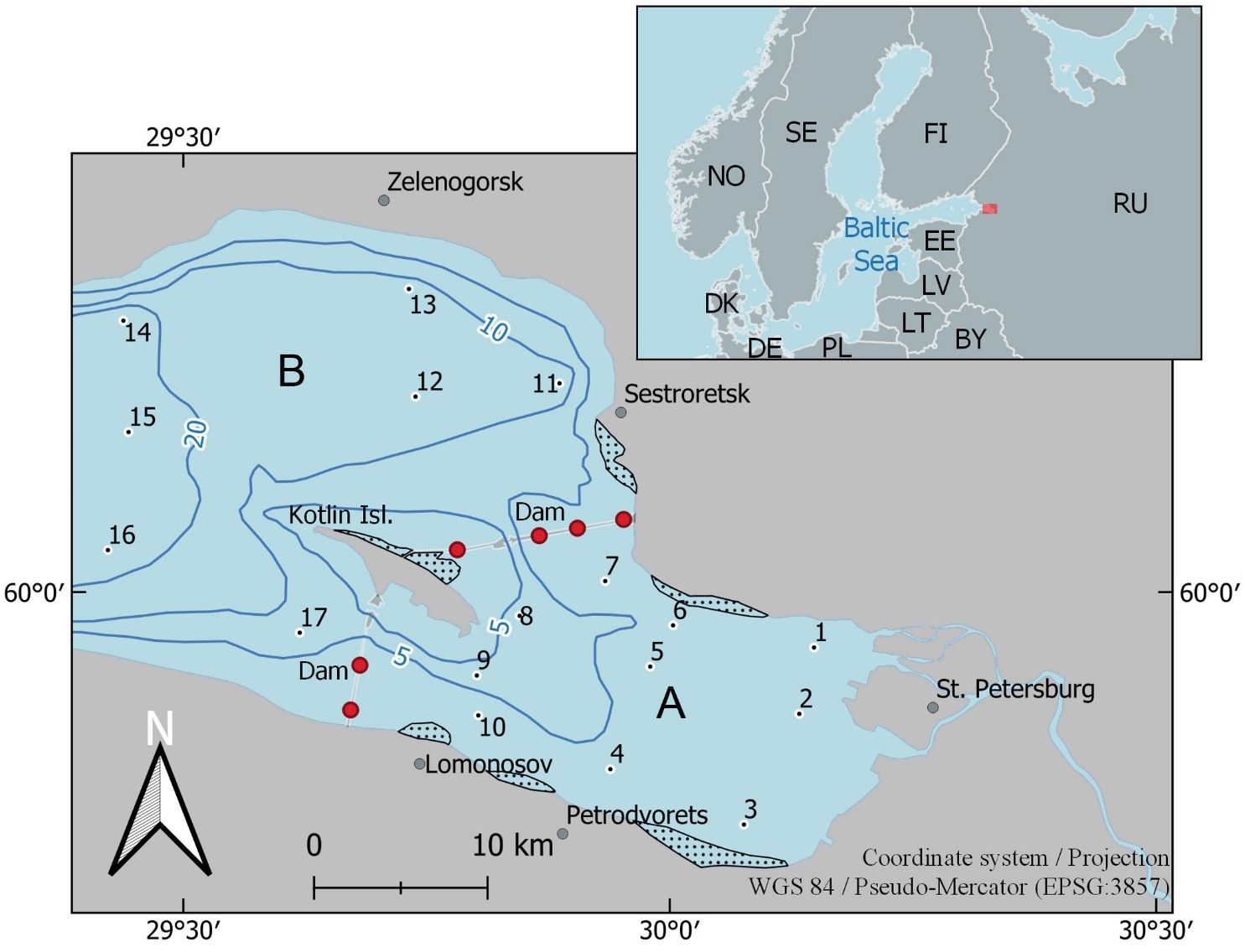
Figure 1 The upper (A) and middle (B) parts of the Neva Estuary with indication of sampling stations in midsummer 2012–2020. Blue lines: isobaths of 5, 10, and 20 m. Areas with dots indicate dense reeds. Dam — the St. Petersburg Flood Protection Facility. Red circles - waters gates in the Dam. Red rectangle in the top block of the map – the location of the Neva Estuary. Two-letter country codes are given according to ISO 3166-1 alpha-2 (International Organization for Standardization (ISO), 2023).

The Neva Estuary is a shallow and non-tidal system, exhibiting a gradual transition from freshwater in the upper part to slightly saline water in the lower part (Golubkov and Golubkov, 2020). Due to its proximity to the 5-million-strong city St. Petersburg, the estuary is subject to significant anthropogenic impacts (Golubkov et al., 2019). To mitigate the risk of flooding, the Flood Protective Facility, consisting of 11 dams, was constructed in the late 1980s, effectively separating the upper part (UP) of the estuary from its middle part (MP) (Figure 1). The UP of the estuary lacks temperature stratification, and the presence of low water transparency and strong currents hinders the development of benthic aquatic vegetation. The MP of the estuary, located between Kotlin Island and the arbitrary boundary of 29°10` E, experiences temperature stratification during summer season. For a comprehensive understanding of ecological characteristics of the Neva Estuary and a detailed description of both its parts, refer to Golubkov and Golubkov (2021).

2.2 Data and methods

In this study, we used data from long-term scientific monitoring of the Neva Estuary ecosystem. The data used for analysis collected in the upper and middle parts of the estuary (Figure 1) during late July-early August 2012–2020. Salinity (S) and temperature (T) were conducted using a CTD90M probe from Sea&Sun Tech (Germany). The concentration of colored dissolved organic matter (CDOM) and chlorophyll a (CHL), as well as turbidity (Turb), were determined using Cyclop-7 sensors connected to a submersible C-6 multi-sensor platform (TurnersDesigns, United States). Prior to measurements, the Cyclop-7 sensors were checked and calibrated using TurnersDesigns solid standard. In the case of CDOM, the Cyclop-7 sensor was additionally calibrated based on the corrections proposed by Downing et al. (2012). Test material of humic substances (HS) derived from typical soils in the Neva Estuary watershed was obtained from the Department of Soil Science and Soil Ecology of St. Petersburg State University. HS solutions were prepared by dissolving 1 g of test material in 1 L of organic-free deionized water, after which it was diluted to several solutions with HS concentration of 0.0005, 0.001, 0.002, 0.003, 0.004, 0.005, 0.007, 0.01 mass percent. Fluorimeter measurements were carried out following the method described by Downing et al. (2012), and the carbon concentration in these solutions was measured using high-temperature catalytic oxidation with Shimadzu TOC-L_CPN/CSN instrument (Shimadzu Scientific Instrument, Japan) based on the method by Bird et al. (2003).

The PAR values were determined using a LiCOR-193SA scalar quantum sensor connected with a tripod to a CTD90M probe and controlled using Sea&Sun Tech software. The LiCOR-193SA sensor was calibrated every 2 years (according to recommendations of manufacture) using spectrophotometer and reference silicon photodiodes traceable to the National Institute of Standards and Technology (NIST).

All probes were programmed to take readings at 1-second intervals. To minimize errors related to waves, the readings were averaged over standard intervals in 10-centimeter increments. The PAR value on the water surface (PAR₀) was taken as 100%, and the decrease in PAR with depth was expressed as a percentage of PAR₀.

The depth at which the PAR value reached 10% of the PAR₀ value was designated as the depth of 10% PAR₀ (D_10%). The depth at which the PAR value reached 1% of PAR₀ was accepted as the depth of the euphotic zone (D_eu). The number of photons reaching this depth (PAR_Deu) was also measured. The Kd(PAR) was calculated from measurements of the amount of incident radiation near the water surface and of the euphotic zone (Kirk, 2011):

$\begin{array}{ll}\text{Kd}(\text{PAR})=-\frac{1}{\text{z}}\text{ln}\frac{{\text{PAR}}_{\mathrm{Due}}}{{\text{PAR}}_0}& \text{Equation 2}\end{array}$

where PAR₀ and PAR_Deu are the PAR just below the surface and at D_eu, respectively.

Data on Kd(PAR) and D_eu were published and discussed earlier (Golubkov and Golubkov, 2023).

The Secchi disk depth (D_sd) was measured using a 30 cm matt white disk from the shaded side of the boat. Since the depth of the Secchi disk and the vertical profile of PAR were measured simultaneously, we were able to determine the proportion of PAR from the water surface reached D_sd (E_sd). The coefficient F was calculated by the transformed Equation 1:

$\begin{array}{ll}\text{F}=\text{Kd}(\text{PAR})\times {\text{D}}_{\text{sd}}& (3)\end{array}$

The concentrations of total suspended matter (SM) and suspended organic matter (SOM) were also determined, as these variables affect the optical properties of the water column. The concentration of SM in water was obtained using a standard gravimetric method (Grasshoff et al., 1999). The SOM concentration was determined using the dichromate oxidation method of a suspension pre-deposited on preheated (1 h, 105°C) and weighed GF/F filters (Grasshoff et al., 1999). Suspended mineral matter (SMM) concentrations were determined by subtracting SOM values from SM values. Water samples for determining SOM and SM were collected using a 2-liter bathometer from the surface, half a meter above the bottom and from three equidistant horizons between them in the UP of the estuary. In the MP of the estuary, samples for SOM and SM were taken from a horizon above the thermocline, which was determined using CTD90M probe. The samples were obtained from the surface, a depth of 0.5 m above the thermocline, and three equidistant horizons. This allowed us to obtain composite samples of 10 l, from which 0.5 l of water was taken for laboratory determination of SOM and SM.

2.3 Statistical analysis and data modeling

The D_sd, D_10%, subtraction value between D_sd and D_10%, and the ratio between D_eu and D_sd were averaged for each station over 2012–2020 and visualized with SURFER 8.0 using the kriging data extrapolation model. A total of 153 data points were used for this visualization, including 18 stations over 9 years.

Untransformed data was used for statistical analysis. Data from stations where the PAR penetration depth was limited by the bottom were excluded from regression analysis, this resulted in a matrix of 89 data points (Supplementary Tables 1S, 2S). Regression analysis was performed in Microsoft Excel. We used the same data set for this analysis as in Golubkov and Golubkov (2023).

Part of the SOM data was missing in 2020; in this regard, we analyzed in principal component analysis, recursive splitting and building of regression trees only data for 2012–2019. Some stations also did not have all indicators. As a result, for principal component analysis, recursive splitting and building of regression trees, we got a final matrix of 67 data lines for each indicator (Supplementary Tables 1S, 3S).

Principal component analysis (PCA), as well as classification and regression tree analysis (CART) were performed using R software (version 4.2.2) (R Core Team, 2023). PCA analysis was applied to elucidate the relationship between the optical characteristics of water and environmental variables, which was performed using the “prcomp” command of the “Stat” package (R Core Team, 2023), and the results were visualized using the “fviz_pca_biplot” command of the package “factoextra” (Kassambara and Mundt, 2020). The script and the full output of principal component analysis are shown in Supplementary Table 4S.

Regression trees were constructed using recursive partitioning of data based on analysis of variance (Breiman, 1984). CART is a prediction algorithm used in machine learning to predict outcomes based on predictor variables. The decision tree construction algorithm was performed from top to bottom by choosing a variable at each step that best splits the set of elements, which is the most commonly used method (Rokach and Maimon, 2005). It explains how the values of the target variable can be predicted based on other values. The goal of CART is to develop a sequence of partitioning rules to split response variable observations (i.e., Secchi disk depths) into relatively small, homogeneous groups of observations using related explanatory variable values. This is a decision tree where each fork is split into a predictor variable and each node at the end has a prediction for the target variable.

In this work, the decrease in the variance of the dependent variable was chosen as a measure of the best solution, for which the analysis of variance was used. This process, which is repeated recursively on each resulting subset, is called recursive partitioning. The recursion is terminated when a subset in a node has the same target variable value, or when the split adds no value to the predictions. This top-down induction of decision trees (TDIDT) process is the most commonly used strategy for learning decision trees from data (Quinlan, 1986).

The tree models were built using the “rpart” command of the “rpart” package (Therneau et al., 2022) using the “anova” partitioning method, i.e. search for a solution with the smallest variance of the dependent variable at the node. The “rpart.plot” command from the “rpart.plot” package (Milborrow, 2022) was used to visualize the regression trees. The script and the full output of CART are shown in Table 5S.

3 Results

3.1 Secchi disk depth

The Secchi disk depth changed seven times in the midsummer, averaging 1.4 m (Table 1). The lowest D_sd values were observed in the coastal area of the UP of the estuary, while the highest values were found at the confluence of the Neva River into the UP of the estuary and in the seaward western region of the MP of the estuary (Figure 2A). The amount of PAR at the Secchi disk depth (E_sd) averaged about 15% of the PAR at the water surface, but the range of E_sd values was from 2 to 45%.

Table 1

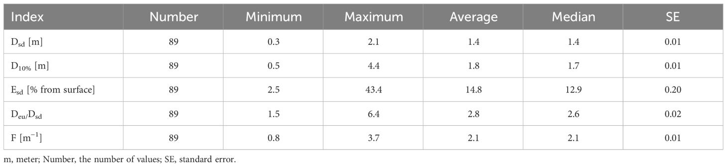
Table 1 The Secchi disk depth (D_sd), the depth at which 10% of the PAR incident the water surface remains (D_10%), the proportion of PAR at the Secchi disk depth (E_sd) of the PAR on the water surface, the ratio of the depth of the euphotic zone to the Secchi disk depth (D_eu/D_sd) and the value of the absorption coefficient of PAR (F).

Figure 2

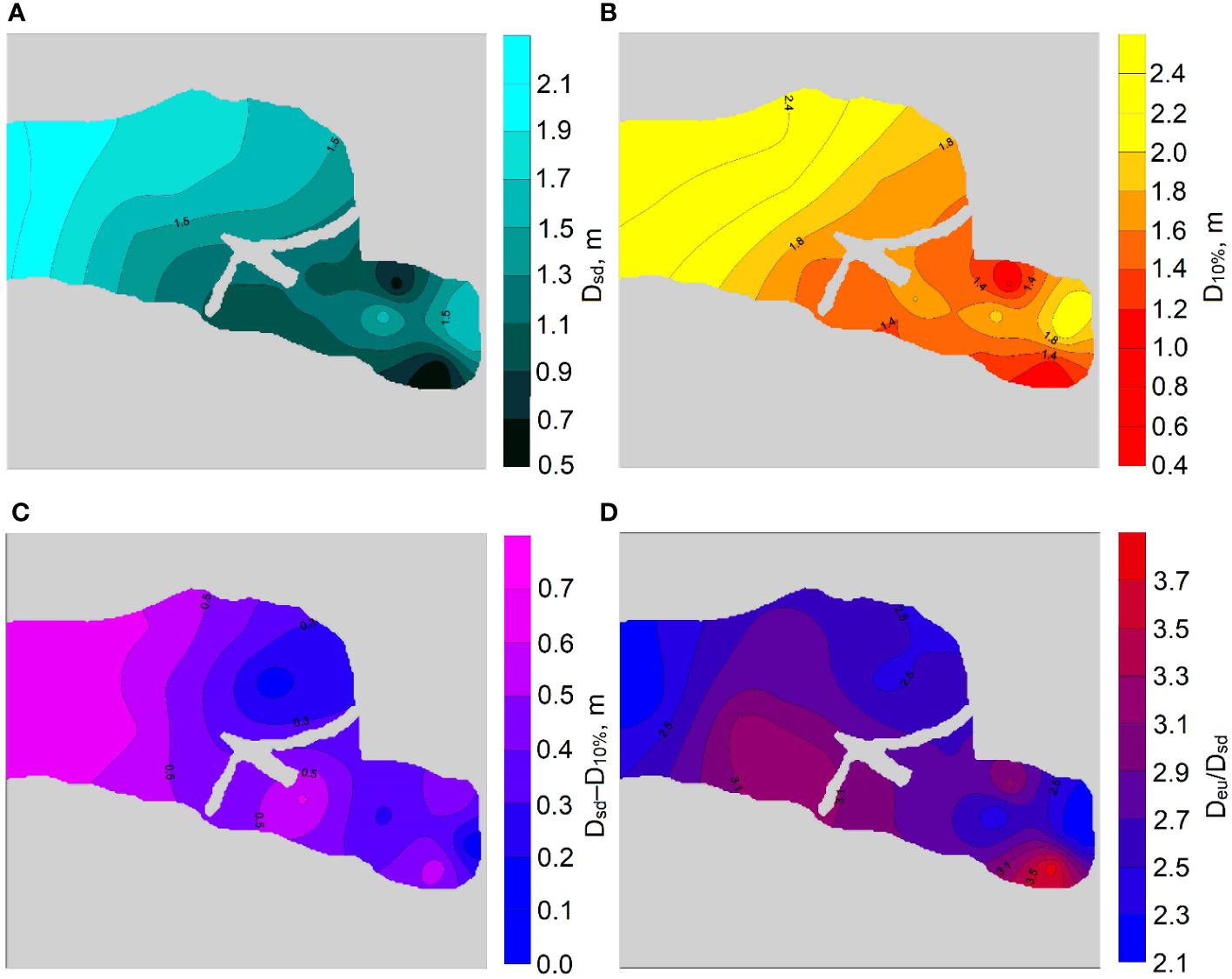
Figure 2 Average values of the Secchi disk depth (D_sd) (A) and the depth at which 10% of the surface PAR remains (D_10%) (B), as well as the difference between D_10% and D_sd (C), and the ratio of the depth of the euphotic zone to the Secchi disk depth (D_eu/D_sd) (D) in midsummer 2012–2020.

The spatial distribution of D_sd and D_10% practically coincide (Figures 2A, B), and regression analysis confirmed a significant relationship between these indicators (Figure 3A). However, D_sd was generally less than D_10% (Table 1, Figures 2C, 3A). The largest differences were observed in the seaward part of the studied water area and in the northwestern UP of the estuary, where D_sd was more than 0.5 m less than D_10% (Figure 2C).

Figure 3

Figure 3 Relationship between the Secchi disk depth (D_sd) and the depth at which 10% of the surface PAR remains (D_10%) (A), and the percentage of the surface PAR at the Secchi disk depth (E_sd) (B). The black line is the trend line of the empirical data, the orange line is the theoretical dependence, where it is assumed that D_10% = D_sd. subscript “T” specifies theoretical data, subscript “E” indicates empirical ones. R² – coefficient of determination.

Although D_sd and D_10% are related, their relationship in the Neva Estuary deviates from the theoretical linear trend (Figure 3A). Instead, a logarithmic dependence of D_sd on D_10% demonstrated the highest coefficient of determination. The theoretical and empirical trend lines closely matched for D_10% values ranging from 1 to approximately 2.5 m, but noticeable divergence occurred for D_10% values below 1 and above 3 m (Figure 3A). In the Neva Estuary, the median E_sd value was 12.9% (Table 1), which is proximity to the theoretical E_sd = 10%. However, E_sd in the Neva Estuary was not constant. We obtained a statistically significant linear relationship between D_sd and E_sd (Figure 3B). This relationship revealed that at low D_sd values, E_sd could reach up to 40% (Figure 3B). Conversely, at the highest D_sd values, E_sd in some cases was less than 5% (Figure 3B).

3.2 Relationship between the Secchi disk depth and the depth of the euphotic zone

The depth of the Secchi disk in the Neva Estuary was, on average, 2.8 times less than the depth of the euphotic zone, while the minimum and maximum values differed four times (Table 1). The diffuse PAR attenuation coefficient was related by a power function to D_sd (Figure 4A). D_sd decreased most strongly at Kd(PAR) values up to 2 m⁻¹, at which D_sd was approximately 0.5 m, and a further increase in Kd(PAR) led to a slight decrease in D_sd (Figure 4A). Although D_sd was significantly linearly related to D_eu, the scatter of D_eu values increased with increasing Secchi disk depth (Figure 4B). For example, with D_sd about 2 m, D_eu could be both 3.5 and 8 m. There was also a significant linear relationship between D_eu/D_sd and E_sd (Figure 4C). At stations where 30-40% of the PAR reached the Secchi disk depth, the D_eu was three to six times greater than the D_sd (Figure 4C).

Figure 4

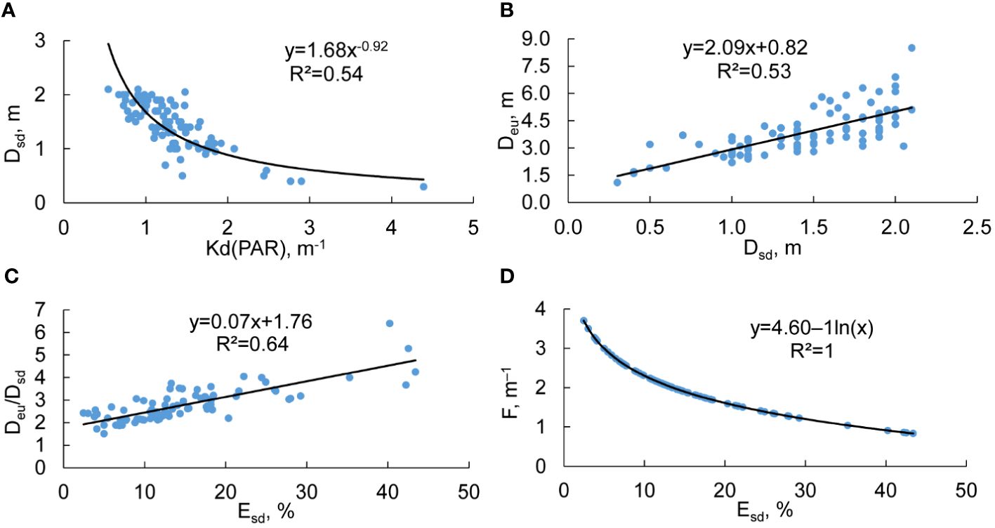
Figure 4 Relationship between the Secchi disk depth (D_sd) and the diffuse PAR attenuation coefficient [Kd(PAR)] in the euphotic layer (A) and the depth of this layer (D_eu) (B); the dependence of D_eu/D_sd ratio (C) and absorbtion coefficient of PAR (F) (D) on the percentage of PAR at the Secchi disk depth (E_sd). R² – coefficient of determination.

The coefficient F showed an inverse proportional relationship with E_sd (Figure 4D). High E_sd values of around 40% corresponded to a F value of approximately 1 m⁻¹, while E_sd values close to 5% resulted in a F value about 4 m⁻¹ (Figure 4D). The spatial distribution of the D_eu/D_sd ratio revealed that, on average, the highest values of the ratio were observed in the southeastern parts of the UP and the MP of the estuary (Figure 2D). This indicates that there was no consistent increasing or decreasing the D_eu/D_sd ratio with distance from the river mouth or from the coast towards the central part of the estuary (Figure 2D). The D_eu/D_sd ratio was related to the F coefficient by a power function (Figure 5). The relationship showed that the D_eu/D_sd ratio reached its maximum when the F coefficient values were at their minimum, which occurred in areas with high Kd(PAR) and low D_sd. Conversely, when Kd(PAR) values were low and D_sd values were high, the D_eu/D_sd ratio was low (Figure 5). In other words, in more transparent waters of the Neva Estuary, the difference between the depth of the euphotic zone and the Secchi disk depth decreased.

Figure 5

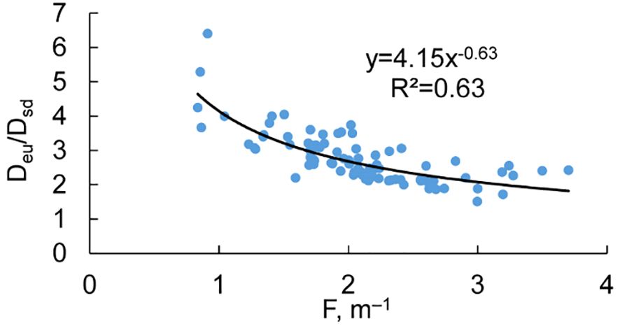
Figure 5 Relationship between the ratio of the depth of the euphotic zone to the Secchi disk depth (D_eu/D_sd) and the absorption coefficient of PAR (F, m⁻¹) in the Neva Estuary in midsummer 2012-2020. R² – coefficient of determination.

3.3 Relationships of environmental variables with the values of the D_eu/D_sd ratio and the coefficient F

The minimum, maximum, mean and median values of the environmental variables used in the statistical analysis are shown in Table 2.

Table 2

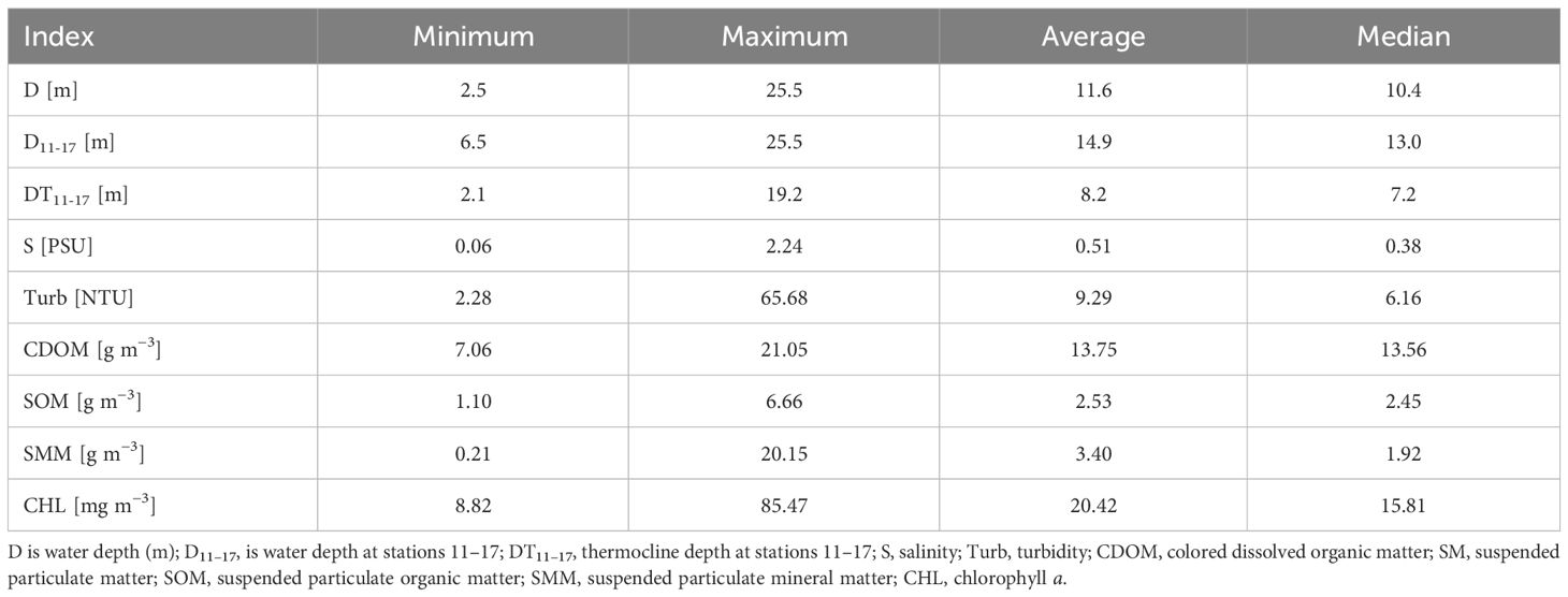
Table 2 Morphometric, physio-chemical, and biological indicators at sampling stations in the Neva Estuary in late July – early August 2012–2020.

Principal component analysis demonstrated that the D_eu/D_sd ratio could exceed the median value of 2.6 for any combination of the studied factors (Figure 6). According to PСA, vectors of turbidity change, SMM concentration, and percent PAR at the Secchi disc depth were positively related to each other and negatively related to CDOM concentration and the values of F coefficient. At the same time, Turb, SMM, and E_sd did not depend on the water area depth (D) and the salinity of the waters, which in this case could be taken as a measure of the distance from the mouth of the Neva River. This suggests that very different values of these indicators can be observed in both the seaward and deeper part of the estuary and in the shallow part near the mouth of the Neva River (Figure 6).

Figure 6

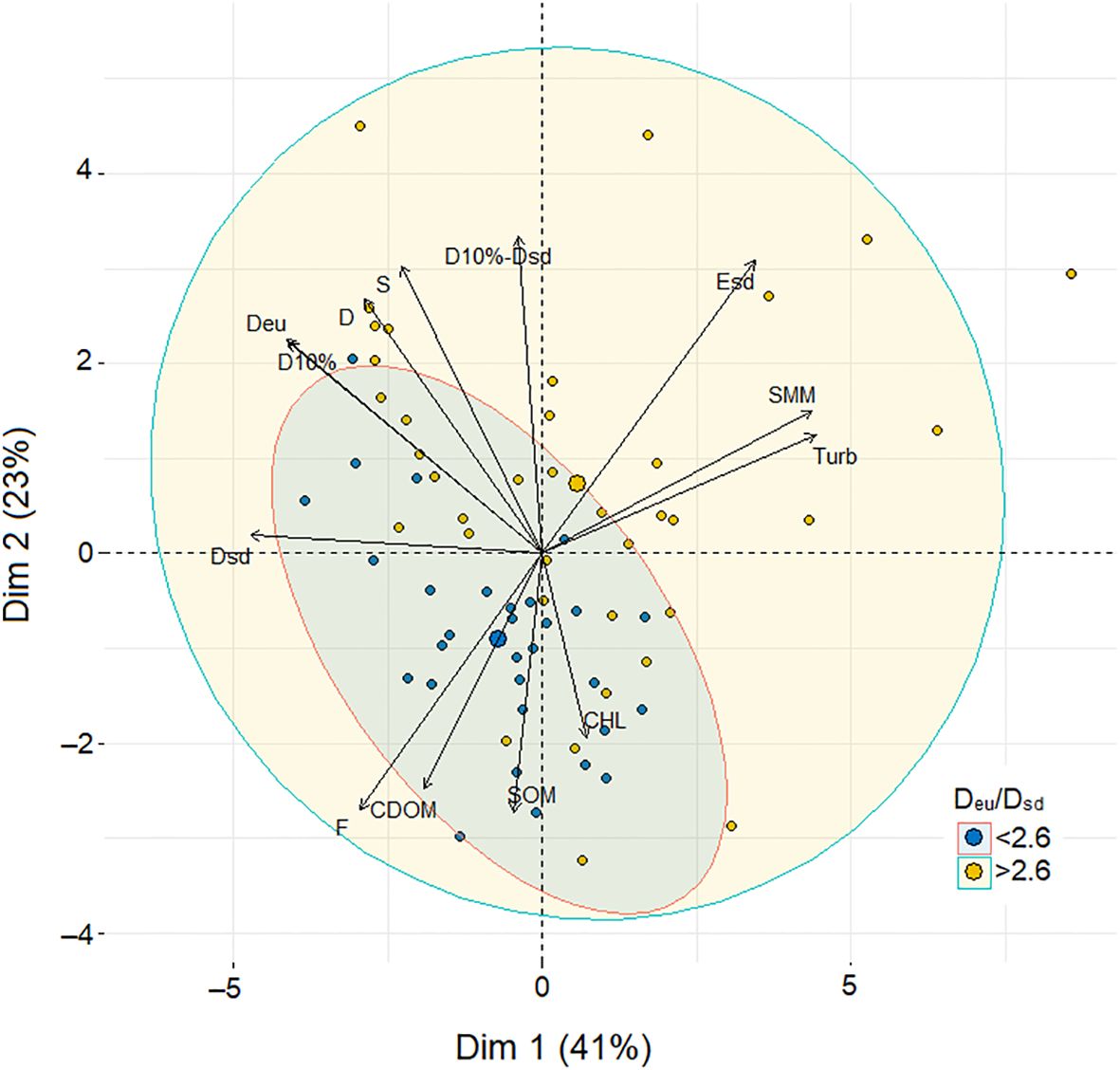
Figure 6 Results of principal component analysis of relationships between water transparency indices and environmental variables. All observation sites are ranked according to the D_eu/D_sd ratio. Yellow dots are observation sites where D_eu/D_sd was less than the median of the entire dataset (<2.6). Blue dots are observation sites where D_eu/D_sd was greater than the median of the entire dataset (>2.6). The contours show the individuals (data points) distribution for each data set in which the D_eu/D_sd ratio was greater than or less than 2.6. The large blue and yellow dots are the centers of the dispersion ellipses for each data set. The arrows show the vectors of changes in the indicators of the optical characteristics of water and environmental variables.

The distribution of D_eu/D_sd values showed more localized changes within the boundaries of D_eu/D_sd<2.6, which was contained within the distribution ellipse of D_eu/D_sd >2.6 (Figure 6). This means that the D_eu/D_sd ratio can be high and low for the same environment variables. It is noteworthy that the vectors of depth and salinity changes in the estuary were elongated along the ellipse D_eu/D_sd < 2.6, which indicates that the D_eu/D_sd ratio can be low both in the seaward and saline part of the estuary and in its shallow freshwater part (Figure 6).

Recursive partitioning based on analysis of variance provided more interpretable results. It revealed that the concentration of mineral suspended matter was the main factor contributing to the variance in D_sd (Figure 7A). When the SMM concentration exceeded 3.9 g m⁻³, the average D_sd was about 0.9 m, whereas it was 1.6 m when the concentration was below 3.9 g m⁻³ (Figure 7A). CDOM concentration and estuary depth were the next significant predictors of D_sd variance. When the SMM concentration was below 3.9 g m⁻³, D became the second most influential factor, while CDOM played this role when the SMM concentration exceeded 3.9 g m⁻³. Additionally, for depths greater than 11 m and SMM concentration below 3.9 g m⁻³, the dispersion of D_sd was significantly determined by chlorophyll a concentration (Figure 7A).

Figure 7

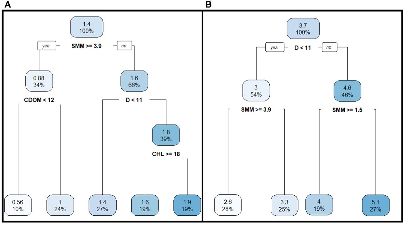
Figure 7 An inverted regression trees for Secchi disk depth (A) and depth of euphotic zone (B) obtained as a result of recursive partitioning of the data set based on the results of the analysis of variance. The numbers inside the block are the average value of the indicator (in meter) shown along with the percentage of cases of the total number of observations. At low values of the indicator, the color of the block is pale; the more saturated the color, the higher the values. The legend below the block is the abbreviated name of the main environmental factor in its units that determines the variance of the array. The numbers show the average values of the main environmental factors influencing D_sd and D_eu; the signs< > are symbols more and less. Yes and No are indicators of compliance or non-compliance with the necessary condition (the value of the influencing factor). The factors that determine the dispersion are arranged in a hierarchical pyramid. The factor at the top of the pyramid is the determining factor for the entire data set and a necessary condition when considering the factors below that determine the variance in certain parts of the entire data set.

In contrast to D_sd, the variance in D_eu values was primarily explained by two predictors: estuary depth and SMM concentration (Figure 7B). Estuary depth was the main environmental factor influencing the dispersion of D_eu. For stations with depths exceeding 11 m and SMM concentration below 1.5 g m⁻³, the average D_eu was around 5 m. In the shallow parts of the estuary, where the depth was less than 11 m and SMM concentration exceeded 3.9 g m⁻³, the average D_eu value was about 2.6 m (Figure 7B). Therefore, although D_sd and D_eu were linearly related (Figure 4B), the set of environmental factors influencing their variance was slightly different (Figure 8), which likely explains the high variability observed in D_eu values at the same D_sd during linear regression (Figure 4B).

Figure 8

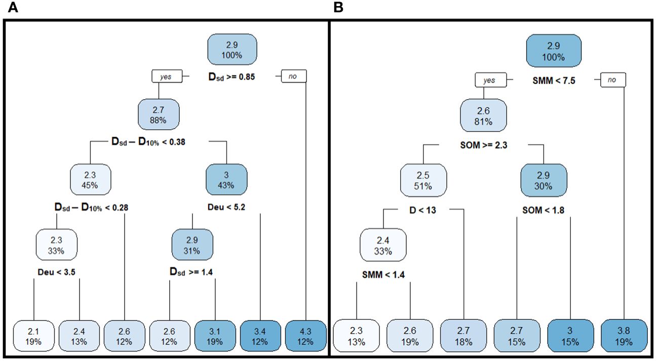
Figure 8 An inverted regression trees for the values of the D_eu/D_sd ratio depending on the optical characteristics of water (A) and environmental factors (B) obtained as a result of recursive partitioning of the data array based on the results of the analysis of variance. The designations are the same as in Figure 7.

The D_eu/D_sd ratio was mainly determined by changes in D_sd rather than D_eu (Figure 8A). The regression tree constructed for the D_eu/D_sd ratio, using environmental factors as predictors, showed that SMM concentration was the primary predictor determining the value of this ratio (Figure 8B). When SMM concentration exceeded 7.5 g m⁻³ and D_sd was below 0.85 m, the D_eu/D_sd ratio was around 4 (Figures 8A, B). A more complex relationship was observed for lower SMM concentrations and higher D_sd values where different combinations of mineral and organic suspended matter concentrations, estuary depth and differences between D_sd and D_10% or D_eu led to similar D_eu/D_sd values (Figure 8).

For example, the average D_eu/D_sd ratio was about 2.7 when:

1. the SMM was below 7.5 g m⁻³, the SOM concentration was greater than or equal to 2.3 g m⁻³, and the depth was above 13 m;

2. the SMM was below 7.5 g m⁻³ and SOM concentration was less than 1.8 g m⁻³, with estuary depth not affecting the variance of D_eu/D_sd ratio (Figure 8B).

The lowest D_eu/D_sd values around 2.0 were observed at concentrations of SMM< 1.4 g m⁻³ and SOM > 2.3 g m⁻³, while the D< 13 m, D_sd > 0.85 m, D_eu< 3.5 m, and D_sd differed from the theoretical D_10% less than 0.28 m (Figures 8A, B). These findings indicate that the calculation of D_eu from D_sd values in estuaries using simple linear regressions is hardly justified, as real data can deviate significantly from theoretical predictions.

The dispersion of the F coefficient, which relates with the optical characteristics of water, was explained by the amount of PAR remaining at the Secchi disk depth. When E_sd was less than or equal to 10% of surface PAR, the averaged F was 2.8 m⁻¹, while it was 1.2 m⁻¹ when E_sd exceeded 20% (Figure 9A).

Figure 9

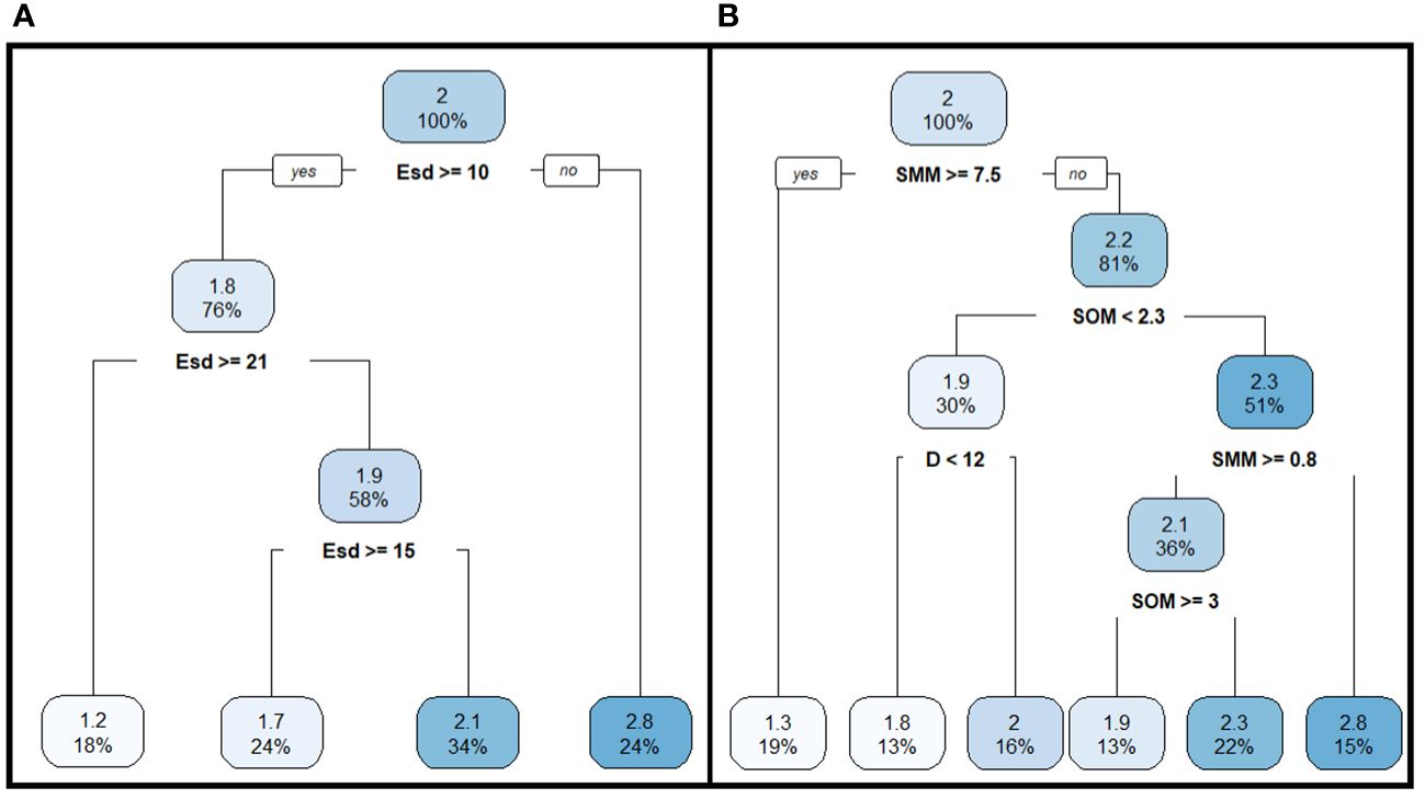
Figure 9 An inverted regression trees for the coefficient F (m⁻¹) depending on the optical characteristic of water (A) and environmental factors (B) obtained by recursive partitioning of the data array based on the results of the analysis of variance. The designations are the same as in Figure 7.

The main predictor associated with low F coefficient and a high D_eu/D_sd ratio was an SMM concentration greater than 7.5 g m⁻³ (Figures 8B, 9B). Conversely, a high F coefficient was observed when the SMM concentration was less than 0.8 g m⁻³, but the SOM concentration was greater than 2.4 g m⁻³; indicating that the organic fraction constituted about 75% of the total suspended matter. It was challenging to predict precise F values based on the studied environmental factors, as different combinations of the same factors led to overlapping F values (Figure 9B). For instance, the mean F value was 1.8 m⁻¹ when the SMM concentration was below 7.5 g m⁻³, SOM concentration was below 2.3 g m⁻³, and depth was less than 12 m. In the deeper parts of the estuary with depths greater than 12 m, this coefficient averaged 2.0 m⁻¹. Similarly, the average F value was 1.9 m⁻¹ when the SMM concentration was less than 7.5 g m^–3, but above 0.8 g m⁻³, and the SOM concentration ranged above 3.0 g m⁻³. Under these conditions, the depth did not significantly influence the variance of the F coefficient. In general, the value of the F coefficient in different parts of the Neva Estuary was determined by a combination of E_sd, SMM, SOM values and, in some cases, the depth of the water area (Figure 9).

Using the CART approach, it was found that the concentration of SMM was the main predictor of E_sd in different parts the estuary. When the SMM concentration exceeded 7.5 g m⁻³, an average of 28% PAR from the surface remained at the Secchi disk depth, significantly higher than the theoretical value of 10% PAR. At SMM concentrations below 7.5 g m⁻³, the variance of the E_sd indicator was determined by various combinations of three variables: depth, SMM concentration, and SOM concentration. The lowest percentage of PAR from the surface at the Secchi disk depth was observed at SOM concentrations greater than 2.3 g m⁻³ and SMM concentrations less than 0.8 g m⁻³ (Figure 10A). Under these conditions, E_sd averaged 7.3%. This suggests that the Secchi disk disappeared from view at a later depth than predicted by the theoretical relationship, where 10% of the PAR value on the water surface should remain at the Secchi disk depth. This case corresponds to the regression points of the D_sd–D_10% relationship located above the orange line in Figure 3A when D_sd>D_10%. Overall, the difference between D_10% and D_sd was mainly determined by water salinity and SMM concentration. At water salinity above 0.73 ‰ and SMM concentrations above 1.8 g m⁻³, the depth at which 10% of the surface PAR remained was 0.94 m greater than the Secchi disk depth (Figure 10B). The smallest difference between these indicators was observed at salinity from 0.34 to 0.73 ‰, while the largest difference occurred in more saline waters (Figure 10B).

Figure 10

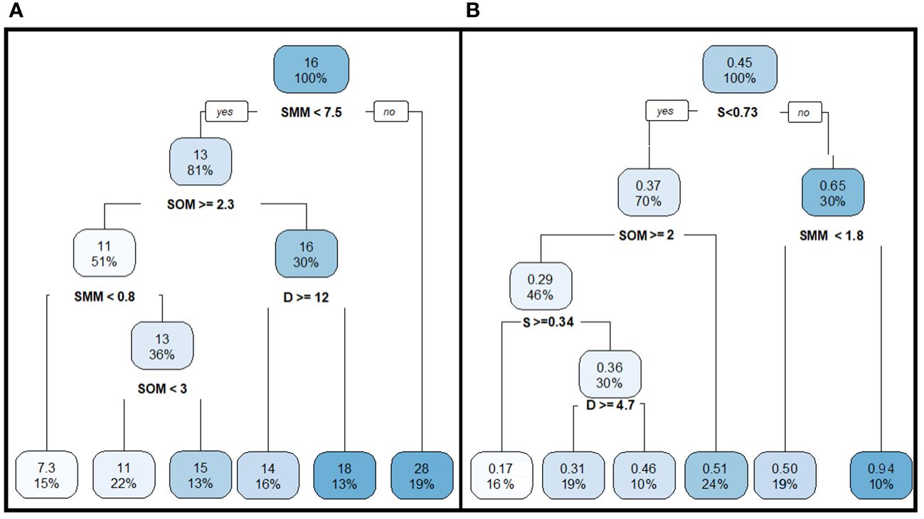
Figure 10 An inverted regression trees for E_sd (%) (A) and the difference between D_10% and D_sd (m) (B) depending on environmental factors, obtained as a result of recursive partitioning of the data array based on analysis of variance. The designations are the same as in Figure 7.

Based on the data, the Secchi disk depth did not show a statistically significant relationship with chlorophyll a concentration in the upper and middle parts of the Neva Estuary (Figure 11A). Therefore, it is difficult to reconstruct historical phytoplankton development solely based on D_sd in the Neva Estuary, as D_sd depends more on water turbidity than phytoplankton biomass (Figure 11B).

Figure 11

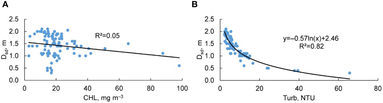
Figure 11 Relationship of Secchi disk depth (D_sd) with chlorophyll a concentration (CHL) (A) and total water turbidity (Turb) (B). R² – coefficient of determination.

4 Discussion

Published data on the Secchi disk depth in the Baltic Sea reveal variations across different regions. The Gulf of Riga shows a lower limit of D_sd at 0.5 m, while the Sea of Bothnia reaches up to 15.3 m (Fleming-Lehtinen and Laamanen, 2012). Harvey et al. (2019) reported similar findings, with minimum D_sd values of 0.5 m near the Swedish coast of the Bothnian Sea and a maximum value of 12.8 m in the Baltic Proper during midsummer. Neumann et al. (2015) found that in the open waters of the Baltic Sea, D_sd ranged from 2.5 to 22 m along the transect from the Bay of Bothnia to the entrance to the North Sea. In the shallow fjords of the Danish Straits, which connect the Baltic and North Seas, D_sd has fluctuated between 2 and 6 m over the past 30 years (Pedersen et al., 2014). Comparing our data with these published findings, it is evident that the upper and middle parts of the Neva Estuary are characterized lower D_sd values (Table 1) compared to the open waters of the Baltic Sea. However, in the Estonian coastal waters of the Gulf of Finland, D_sd periodically reached as low as 0.2 m, likely due to dredging activities in the area (Liblik and Lips, 2011). Similarly, in the Neva Estuary, hydrotechnical work was also periodically carried out, and the minimum values of D_sd (Table 1) were timed to coincide with these works, when a lot of suspended particles entered the water column, and negatively affected the productivity and species richness of phytoplankton in the estuary (Golubkov and Golubkov, 2022; Golubkov et al., 2023).

The theoretical understanding is that the Secchi disk disappears from view at a depth where 10% of the surface PAR remains (Preisendorfer, 1986; Kirk, 2011). This has been confirmed by studies in the Atlantic coastal waters at depths greater than 10 m (Lee et al., 2018). However, according to numerous empirical data, the Secchi disk becomes invisible to the human eye at depths where 5 to 40% of the surface PAR reaches, with an average of about 18% (Koenings and Edmundson, 1991). In the Neva Estuary, E_sd fluctuated even more widely, from 2.5 to 43.5%, with an average value of about 15% (Table 1), which exceeds the theoretical calculated 10% value. The largest difference between D_10% and D_sd was observed in the zones of hydrotechnical works, where suspended particles concentration was exceptionally high (Figure 2C, Golubkov and Golubkov, 2022; Golubkov et al., 2023). In these areas with SMM concentrations above 1.8 g m⁻³, the Secchi disk became invisible almost a meter before reaching the D_10% (Figure 10B).

Contrary to these observations, Bowers et al. (2020) reported that at suspended matter concentrations greater than 20 g m⁻³, the classical theory (Holmes, 1970; Preisendorfer, 1986) underestimates the depth of the Secchi disk because it suggests that diffuse sunlight falling on the disk is reflected back to the observer’s eye along the most direct route, as a beam. However, actually, in turbid waters, some of the light reflected by the disk returns to the eye as diffuse light and increases its brightness to the human eye. As a result, the Secchi disk is visible at greater depths (by a factor of up to 4) than predicted by this theory (Bowers et al., 2020). Our data indicate that under certain conditions, this effect may also occur in the Neva Estuary, in the case when the Secchi disk disappeared later than the D_10%, when an average of 7.3% of the PAR remained at the D_sd from its value on the water surface (Figure 10A). In such cases, D_eu/D_sd ratio was 2.3 (Figure 8B), that is very closer to classical average 2.4 for all world waters (Lee et al., 2018). This was observed at relatively low SMM concentrations but close to average SOM concentrations (Figure 10A, Table 2). However, in most cases, the Secchi disk disappeared much earlier than reaching the D_10% (Table 1, Figures 2C, 10). This phenomenon is likely due to the high content of CDOM in the waters of the Neva Estuary (Table 2, Golubkov and Golubkov, 2023) compared to open ocean waters (Kratzer and Moore, 2018). According to Bowers et al. (2020), photons reflected from the Secchi disk can be absorbed strongly by the CDOM on their way back to the water surface. Under such conditions, the eye of the researcher does not distinguish the disk well and, as a result, D_10% greatly exceeds D_sd.

In the Chesapeake Bay (USA), the Secchi disk depth increased as the water salinity increased (Testa et al., 2019). A similar spatial distribution of D_sd and D_10% was also observed in the Neva Estuary (Figures 2A, B). However, the difference between these indicators sometimes approached one meter (Figure 10A), and there was no consistent confinement of this difference to specific parts of the part of the estuary (Figure 2C). Although, in general, this difference increased with distance from the mouth of the Neva River, increasing salinity and depth (Figures 2C, 6, 10B), a large difference between these indicators was also observed in some parts of the upper part of the estuary (Figure 2C). In the Neva Estuary, salinity did not affect D_sd (Figure 7A), but was a significant predictor of the difference between D_10% and D_sd. When the water salinity was above 0.73 ‰ this difference was greater, and when it was less, the difference was smaller (Figure 10A). However, this is explained not so much by the salinity of the water or the remoteness from the river mouth, but rather by the construction of port infrastructure that increase the SMM concentration in the middle part of the estuary, where the salinity was higher than in its upper part (Golubkov and Golubkov, 2022; Golubkov et al., 2023). This demonstrates that anthropogenic factors can also influence the difference between D_10% and D_sd.

Similar to other regions in the Baltic Sea (Neumann et al., 2015), our data show that prediction and reconstruction of Kd(PAR) and D_eu in the Neva Estuary based on D_sd data is possible. This is supported by the statistically significant power-law relationship between Kd(PAR) and D_sd (Figure 4A), as well as the linear relationship between D_sd and D_eu (Figure 4B). The significant correlation coefficients indicate that changes in Kd(PAR), D_eu, and D_sd occurred concurrently in the estuary, and these indicators changed synchronously by approximately 50%. This finding aligns with the long-standing use of D_sd to determine the penetration depth of PAR (Fleming-Lehtinen and Laamanen, 2012; Aas et al., 2014). However, the 50% uncertainty of the obtained regressions (Figures 4A, B) imposes certain restrictions on their use when accurate and relatively small-scale estimates are needed. Modeling the relationship between the Secchi disk depth and Kd(PAR) in various oceanic regions has shown inconsistent results, indicating that the relationship between these indicators is not straightforward and can be influenced by multiple factors (Castillo-Ramírez et al., 2021). Caution should be exercised when using D_sd to calculate Kd(PAR) due to the difficulty in obtaining stable and interpretable results. For large-scale comparisons, the spread of values, as observed in Fleming-Lehtinen and Laamanen (2012) for different zones of the Baltic Sea, may not be critical. Nevertheless, when examining a specific depth range, such as up to 20 meters, the scatter of points can be substantial, and a reliable relationship may not be clearly visible, as seen in the study by Nishijima et al. (2016) in the Seto Inland Sea, Japan.

In the open waters of the Baltic Sea and the Neva Estuary, the Secchi disk depth was related by a power law to Kd(PAR) with close coefficient values (Figure 4A, Neumann et al., 2015). The coefficient of proportionality in the equation for the Baltic waters was 1.61, against 1.68 in the Neva Estuary, and the exponent was −0.94 and −0.92, respectively. However, the range of Kd(PAR) and D_sd values for which these equations were obtained differed significantly. According to Neumann et al., 2015, in the open waters of the Baltic Sea from the Bothnian Bay to the entrance of the North Sea, Kd(PAR) varied from about 0.04 to 0.94 m⁻¹, and D_sd from 3 to 24 m. In the Neva Estuary Kd(PAR) ranged from 0.54 to 9.21 m⁻¹ (Golubkov and Golubkov, 2023) and D_sd from 0.3 to 2 m (Table 1). The similarity of the coefficients of these equations to each other means that both dependencies are valid for both coastal and open waters of the Baltic Sea. The power equations of dependences Kd(PAR) - D_sd with completely different coefficients were obtained for lakes located in the catchment area of the Baltic Sea (Paavel et al., 2008; Ficek and Zapadka, 2010).

Although the equations obtained for the Baltic well describe the average dependences of Kd(PAR) on D_sd, the spread of the measured values of D_sd used to calculate the equations can reach 3-4 times (Figure 4A, Neumann et al., 2015). This variation arises because D_sd can be influenced by different environmental factors, and the same D_sd values in different regions of the Baltic Sea may not always correspond to the same environmental conditions (Harvey et al., 2019). Our results confirm this opinion. Principal component analysis, in which the entire data set was analyzed as a single vector, did not allow us to separate the data by the D_eu/D_sd ratio in the Neva Estuary depending on environmental variables (Figure 6). Modeling by building regression trees based on recursive partitioning of the data arrays made it possible to identify combinations of factors that affect the D_eu/D_sd ratio, but showed that combinations of different factors can lead to the same values of this ratio (Figure 8).

The same result was obtained for the PAR absorption coefficient F, used in the Equation 1 for calculating Kd(PAR) from D_sd measurements (Figure 10). Recursive partitioning of the data array showed that, on average, F was 2.8 for E_sd<10%, 2.1 for E_sd from 10 to 14%, 1.7 for E_sd between 15 to 20% and 1.2 for E_sd≥21% of the PAR on the water surface (Figure 9A). These results roughly align with theoretical calculations that associate 7.6% of the PAR on the surface with an F value of 2.57 and the D_eu/D_sd ratio of 1.79 (Preisendorfer, 1986) and are consistent with the finding of Poole and Atkins (1929), who reported an average F value of 1.7 for an average E_sd of 15%. In our study, the D_eu/D_sd ratio calculated according equation in Figure 5 was 2.2 if the F value was 2.8 m⁻¹ and the E_sd value was less than 10% of the surface PAR (Figures 6, 9A). This was observed when the SMM concentration was less than 0.8 g m⁻³, the SOM concentration was greater than 2.3 g m⁻³, and the depth of estuary was less than 13 m (Figures 8B, 9A, 10A). No other environmental variables emerged as predictors of these indicators in the Neva Estuary.

Our average F value of 2.1 m⁻¹ for the Neva Estuary (Table 1) coincides with the middle of its range from 1.7 to 2.3 m⁻¹ reported for the Baltic Sea (HELCOM, 2002). However, the range of fluctuations in the F value in the Neva Estuary is wider than according to the HELCOM data for other areas of the Baltic Sea. The lowest F value of 0.8 m⁻¹ is significantly lower (Table 1) than the proposed F value for turbid water estuaries (1.4 m⁻¹) (Holmes, 1970) and the average F value of 1.4 m⁻¹ obtained from statistical analysis of data from 1419 Chinese lakes (Zhang et al., 2020). On the other hand, the upper limit of the F range in the Neva Estuary is 3.7 m⁻¹ (Table 1), which is close to the maximum F values observed in lakes with colored water (Koenings and Edmundson, 1991). This shows that in estuaries the range of fluctuations in the optical characteristics of water and the depth of penetration of light into the water column are higher than in open sea waters and lakes, which is apparently a common feature of estuaries as water bodies with a complex dynamic water structure (Emelyanov, 2005; Bianchi, 2007).

It is believed that F increases with decreasing salinity in the Baltic Sea, and based on this opinion, it is concluded that the value of the coefficient F is a function of continental CDOM runoff (Kratzer et al., 2003; Pierson et al., 2008). In the Neva Estuary, changes in the F coefficient were positively related with CDOM concentration (Figure 6), but the values could differ or overlap depending on the combination of mineral and organic suspended matter concentrations (Figure 9B), whose changes can be caused by both natural and anthropogenic factors (Golubkov and Golubkov, 2021, 2022). Therefore, the Secchi disk depth in the Neva Estuary was a function of many indicators affecting the water turbidity, but not just one, such as chlorophyll a concentration, which did not show a statistically significant relationship with D_sd (Figure 11A). This was quite expected, since in the rather shallow Neva Estuary, where bottom sediments are easily stirred up in the water column in windy weather, suspended mineral matter was the main predictor of both the Secchi disk depth (Figure 7) and the depth of the euphotic zone (Figure 7, Golubkov and Golubkov, 2023).

The values of the F coefficient and the D_eu/D_sd ratio in the Neva Estuary were closely related (Figure 5). The D_eu/D_sd ratio decreases at high F values (Figure 5) and SMM concentrations above 7.5 g m⁻³ (Figure 8B, 9B). At the same time, in the middle of the range of their values, F and D_eu/D_sd showed a more complex dependence on environmental factors and optical characteristics of water, since different combinations of environmental variables led to the same or intersecting values of F and D_eu/D_sd (Figure 8, 9). In this regard, it cannot be stated without alternative that with an increase, for example, in the concentration of SMM, the coefficient F will consistently decrease, and the D_eu/D_sd ratio will increase. The reason for this may be that estuaries are zones where continental waters mix with marine waters, and as a result, countercurrents are formed and changes in biogeochemical cycles are observed. They include changes in the behavior of both suspended and dissolved substances, sorption and desorption processes, flocculation and sedimentation (Emelyanov, 2005; Bianchi, 2007). All this leads to various combinations of numerous environmental factors.

The D_eu/D_sd ratio and the F coefficient correlate with the PAR remaining at the depth of the disappearance of the white Secchi disk from the observer’s view (Figures 4C, D). In addition, although the Secchi disk depth and the euphotic zone depth are linearly related, there is a significant scatter of points from the trend line (Figure 4B). This suggests that the D_eu/D_sd ratio and F values are also depend on how the human eye perceives the contrast of the Secchi disk. Regression trees conducted separately for D_sd and D_eu indicate that the predictor sets for these indicators do not exactly match (Figure 7). Although for both indicators, the concentration of mineral suspended matter and the depth of the estuary were significant predictors (Figure 7, Golubkov and Golubkov, 2023), for Secchi disk depth, as in Testa et al., 2019, CDOM concentration and chlorophyll a concentration were also significant (Figure 7A). In other words, various admixtures in the water have a greater impact on the visibility of the white disk and, to a lesser extent, on the actual depth of the euphotic zone as measured by PAR sensors. The disk disappears from the field of view when the contrast drops to a critical value, after which the eye of the researcher can no longer distinguish the disk from the background. CDOM and suspensions in water change the contrast and affect the perception of the disc by the human eye (Bowers et al., 2020). For example, studies conducted in a small eutrophic reservoir located on the northern coast of the Neva Estuary showed that at turbidity below 20 NTU, the Secchi disk clearly distinguished differences in water transparency, but when Turb exceeded 40 NTU, D_sd remained virtually unchanged with further increases in chlorophyll a (Golubkov and Golubkov, 2024).

Lee et al. (2018) suggest using a D_eu/D_sd ratio of 3.5 versus the classic 2.4. Our data show that this ratio is reasonable for calculations in the Neva Estuary, but only at high SMM concentrations (Figure 8B). This is the difference between our data and the data of Lee et al. (2018), where the D_eu/D_sd ratio was mainly influenced by the concentration of chlorophyll a. However, in lakes, the high D_eu/D_sd value of 3.5 is characteristic of turbid glacial lakes with high amounts of suspended mineral particles (Koenings and Edmundson, 1991). This also suggests that the same D_eu/D_sd ratios can be caused by different environmental factors, and it is not so easy to choose which ratio to take in estuaries for the transition from D_sd to D_eu (Figure 8), for example, to calculate the plankton primary production. A study of the lakes of Alaska showed that using the Secchi disk, one can reliably determine the depth of light penetration in large clear lakes with low color and suspended matter concentration (LaPerriere and Edmundson, 2000). However, in lakes with the most complex optical characteristics of water, the scatter of values in the dependence of D_sd on Kd(PAR) increases significantly. Similarly, predicting the depth of seagrass distribution in the turbid Roskilde Fjord Estuary using the Secchi disk or Kd(PAR) gave a difference in the D_10% of 0.5 to 1.5 m (Pedersen et al., 2014).

The Secchi disk depth is included in the list of key indicators for assessing eutrophication and nutrient pollution in the Baltic Sea, since chlorophyll a concentration is generally inversely proportional to the value of D_sd (Fleming-Lehtinen and Laamanen, 2012; HELCOM, 2018). However, in Fleming-Lehtinen and Laamanen (2012), at D_sd values less than 5 m, the scatter in the chlorophyll a concentration is very large. For example, at D_sd about 3 m, chlorophyll a concentration varied by an order of magnitude from 3 to 30 mg m⁻³. Our data were obtained in the D_sd range from 0.3 to 2 m (Table 1) in which this dependence does not seem to work. In the UP and MP of the Neva Estuary, we did not obtain a reliable relationship between chlorophyll a and Secchi disk depth (Figure 11A).

In summary, given the complexity and variability of the factors that influence the relationship between the Secchi disk depth and the optical characteristics of water, this indicator should be used with caution for ecological studies and assessments of the degree of water eutrophication. Studies conducted in the Neva Estuary showed that to ensure the reliability of using the Secchi disk to determine the optical characteristics of water, more detailed knowledge is needed about the effect of the amount and combination of various impurities and forms of suspended matter on the Secchi disk depth. Obviously, in order to reliably interpret the data and determine from D_sd, for example, the depth of the euphotic zone, instead of linear regressions, it is necessary to apply more complex models, using machine learning and neural connections, which are now beginning to be actively developed, e.g., Khanna et al. (2022), Zhang et al. (2022), Lin et al. (2022). In order to establish region-specific relationships between D_sd, Kd(PAR) and D_eu/D_sd ratio, it would be beneficial to conduct benchmark determinations of PAR at the Secchi disk disappearance depth in different regions with specific combinations of environmental variables. This would contribute to improve the accuracy of eutrophication assessments and the reconstruction of historical phytoplankton productivity based on D_sd data.

Data availability statement

The original contributions presented in the study are included in the article/Supplementary Material. Further inquiries can be directed to the corresponding author.

Author contributions

MG: Conceptualization, Data curation, Formal Analysis, Investigation, Methodology, Resources, Software, Supervision, Validation, Visualization, Writing – original draft. SG: Conceptualization, Data curation, Formal Analysis, Investigation, Methodology, Resources, Software, Supervision, Validation, Visualization, Writing – original draft.

Funding

The author(s) declare financial support was received for the research, authorship, and/or publication of this article. The study was supported by Zoological Institute RAS (project 122031100274-7).

Acknowledgments

We would like to thank the three reviewers for their constructive comments that significantly improved the early version of the manuscript.

Conflict of interest

The authors declare that the research was conducted in the absence of any commercial or financial relationships that could be construed as a potential conflict of interest.

Publisher’s note

All claims expressed in this article are solely those of the authors and do not necessarily represent those of their affiliated organizations, or those of the publisher, the editors and the reviewers. Any product that may be evaluated in this article, or claim that may be made by its manufacturer, is not guaranteed or endorsed by the publisher.

Supplementary material

The Supplementary Material for this article can be found online at: https://www.frontiersin.org/articles/10.3389/fmars.2024.1265382/full#supplementary-material

References

Aas E., Høkedal J., Sørensen K. (2014). Secchi depth in the Oslofjord–Skagerrak area: Theory, experiments and relationships to other quantities. Ocean. Sci. 10, 177–199. doi: 10.5194/os-10-177-2014

CrossRef Full Text | Google Scholar

Angradi T. R., Ringold P. L., Hall K. (2018). Water clarity measures as indicators of recreational benefits provided by U.S. lakes: Swimming and aesthetics. Ecol. Indic. 93, 1005–1019. doi: 10.1016/j.ecolind.2018.06.001

PubMed Abstract | CrossRef Full Text | Google Scholar

Bianchi T. S. (2007). Biogeochemistry of estuaries (Oxford: Oxford University Press).

Google Scholar

Bird S. M., Fram M. S., Crepeau K. L. (2003). Method of analysis by the U.S. Geological Survey California District Sacramento Laboratory—Determination of dissolved organic carbon in water by high temperature catalytic oxidation, method validation, and quality-control practices. In Open–file report 03-366; U.S. Geological Survey: Sacramento, USA, 2003. Available at: http://pubs.usgs.gov/of/2003/ofr03366/text.html (Accessed March 10, 2024).

Google Scholar

Bowers D. G., Roberts E. M., Hoguane A. M., Fall K. A., Massey G. M., Friedrichs C. T. (2020). Secchi disk measurements in turbid water. J. Geophys. Res.: Oceans. 125, e2020JC016172. doi: 10.1029/2020JC016172

CrossRef Full Text | Google Scholar

Boyce D. G., Worm B. (2015). Patterns and ecological implications of historical marine phytoplankton change. Mar. Ecol. Prog. Ser. 534, 251–272. doi: 10.3354/meps11411

CrossRef Full Text | Google Scholar

Breiman L. (1984). Classification and Regression Trees. 1 st Edition (New York: Routledge). doi: 10.1201/9781315139470

CrossRef Full Text | Google Scholar

Carlson R. E. (1977). A trophic state index for lakes. Limnol. Oceanogr. 22, 361–369. doi: 10.4319/lo.1977.22.2.0361

CrossRef Full Text | Google Scholar

Castillo-Ramírez A., Santamaría-del-Ángel E., González-Silvera A., Frouin R., Sebastiá-Frasquet M.-T., Tan J., et al. (2021). A new algorithm to estimate diffuse attenuation coefficient from Secchi disk depth. J. Mar. Sci. Eng. 8, 558. doi: 10.3390/jmse8080558

CrossRef Full Text | Google Scholar

Downing B. D., Pellerin B. A., Bergamaschi B. A., Saraceno J. F., Kraus T. E. C. (2012). Seeing the light: The effects of particles, dissolved materials, and temperature on in situ measurements of DOM fluorescence in rivers and streams. Limnol. Oceanogr. Methods 10, 767–775. doi: 10.4319/lom.2012.10.767

CrossRef Full Text | Google Scholar

Effler S. W., Strait C., O’Donnell D. M., Effler A. J. P., Peng F., Prestigiacomo A. R., et al. (2017). A mechanistic model for Secchi disk depth, driven by light scattering constituents. Water Air. Soil pollut. 228, 153. doi: 10.1007/s11270-017-3323-7

CrossRef Full Text | Google Scholar

Emelyanov E. M. (2005). The Barrier zones in the oceans (Berlin: Springer-Verlag). doi: 10.1007/b137218

CrossRef Full Text | Google Scholar

Ficek D., Zapadka T. (2010). Variability of bio-optical parameters in Lake Jasień Północny and Lake Jasień Południowy. Limnological. Rev. 10, 67–76. doi: 10.2478/v10194-011-0008-2

CrossRef Full Text | Google Scholar

Fleming-Lehtinen V., Laamanen M. (2012). Long-term changes in Secchi depth and the role of phytoplankton in explaining light attenuation in the Baltic Sea. Estuarine. Coast. Shelf. Sci. 102–103, 1–10. doi: 10.1016/j.ecss.2012.02.015

CrossRef Full Text | Google Scholar

Golubkov M., Golubkov S. (2020). Eutrophication in the Neva Estuary (Baltic Sea): response to temperature and precipitation patterns. Mar. Freshw. Res. 71, 583–595. doi: 10.1071/MF18422

CrossRef Full Text | Google Scholar

Golubkov M., Golubkov S. (2021). Relationships between northern hemisphere teleconnection patterns and phytoplankton productivity in the Neva Estuary (Northeastern Baltic Sea). Front. Mar. Sci. 8. doi: 10.3389/fmars.2021.735790

CrossRef Full Text | Google Scholar

Golubkov M., Golubkov S. (2022). Impact of the construction of new port facilities on primary production of plankton in the Neva estuary (Baltic Sea). Front. Mar. Sci. 9. doi: 10.3389/fmars.2022.851043

PubMed Abstract | CrossRef Full Text | Google Scholar

Golubkov M., Golubkov S. (2023). Photosynthetically active radiation, attenuation coefficient, depth of the euphotic zone, and water turbidity in the Neva estuary: relationship with environmental factors. Estuaries. Coasts. 46, 630–644. doi: 10.1007/s12237-022-01164-9

CrossRef Full Text | Google Scholar

Golubkov M. S., Golubkov S. M. (2024). Secchi disk depth or turbidity, which is better for assessing environmental quality in eutrophic waters? A case study in a shallow hypereutrophic reservoir. Water 16, 18. doi: 10.3390/w16010018

CrossRef Full Text | Google Scholar

Golubkov S. M., Golubkov M. S., Tiunov. A. V. (2019). Anthropogenic carbon as a basal resource in the benthic food webs in the Neva Estuary (Baltic Sea). Mar. pollut. Bull. 146, 190–200. doi: 10.1016/j.marpolbul.2019.06.037

PubMed Abstract | CrossRef Full Text | Google Scholar

Golubkov M. S., Nikulina V. N., Golubkov S. M. (2023). Impact of the construction of new port facilities on the biomass and species composition of phytoplankton in the Neva estuary (Baltic Sea). J. Mar. Sci. Eng. 11, 32. doi: 10.3390/jmse11010032

CrossRef Full Text | Google Scholar

Grasshoff K., Ehrhardt M., Kremling K. (1999). Methods of Seawater Analysis, 3rd, completely revised and extended edition (New York: Wiley-VCH).

Google Scholar

Guo J., Lu J., Zhang Y., Zhou C., Zhang S., Wang D., et al. (2022b). Variability of chlorophyll-a and Secchi disk depth, (1997–2019) in the Bohai Sea based on monthly cloud-free satellite data reconstructions. Remote Sens. 14, 639. doi: 10.3390/rs14030639

CrossRef Full Text | Google Scholar

Guo J., Nie Y., Sun B., Lv X. (2022a). Remote sensing of transparency in the China seas from the ESA-OC-CCI data. Estuarine. Coast. Shelf. Sci. 264, (107693). doi: 10.1016/j.ecss.2021.107693

CrossRef Full Text | Google Scholar

Hall J. R. O., Yackulic C. B., Kennedy T. A., Yard M. D., Rosi-Marshall E. J., Voichick N., et al. (2015). Turbidity, light, temperature, and hydropeaking control primary productivity in the Colorado River, Grand Canyon. Limnol. Oceanogr. 60, 512–526. doi: 10.1002/lno.10031

CrossRef Full Text | Google Scholar

Harvey E. T., Walve J., Andersson A., Karlson B., Kratzer. S. (2019). The effect of optical properties on Secchi depth and implications for eutrophication management. Front. Mar. Sci. 5. doi: 10.3389/fmars.2018.00496

CrossRef Full Text | Google Scholar

HELCOM (2002) Manual for the Marine Monitoring in the COMBINE program of HELCOM, ANNEX C-5 Phytoplankton Primary Production. Available online at: http://sea.helcom.fi/Monas/CombineManual2/PartC/anxc5.html.

Google Scholar

HELCOM (2018). “State of the Baltic Sea – Second Helcom holistic assessment 2011-2016,” in Baltic Sea Environment proceedings 155. Available at: https://helcom.fi/wp-content/uploads/2019/08/Water-clarity-HELCOM-core-indicator-2018.pdf.

Google Scholar

Holmes R. W. (1970). The Secchi disk in turbid coastal zones. Limnol. Oceanogr. 15, 688–694. doi: 10.4319/lo.1970.15.5.0688

CrossRef Full Text | Google Scholar

Idris M., Siang H. L., Amin R., Sidik M. J. (2022). Two-decade dynamics of MODIS-derived Secchi depth in Peninsula Malaysia waters. J. Mar. Syst. 236, 103799. doi: 10.1016/j.jmarsys.2022.103799

CrossRef Full Text | Google Scholar

International Organization for Standardization (ISO) (2023) Country Codes –ISO 3166. Available online at: https://www.iso.org/iso-3166-country-codes.html (Accessed July 18, 2023).

Google Scholar

Jacobs P., Kromkamp J. C., van Leeuwen S. M., Philippart C. J. M. (2020). Planktonic primary production in the western Dutch Wadden Sea. Mar. Ecol. Prog. Ser. 639, 53–71. doi: 10.3354/meps13267

CrossRef Full Text | Google Scholar

Kahru M., Bittig H., Elmgren R., Fleming V., Lee Z., Rehder G. (2022). Baltic Sea transparency from ships and satellites: centennial trends. Mar. Ecol. Prog. Ser. 697, 1–13. doi: 10.3354/meps14151

CrossRef Full Text | Google Scholar

Kassambara A., Mundt F. (2020) factoextra: Extract and Visualize the Results of Multivariate Data Analyses. Available online at: https://cran.r-project.org/web/packages/factoextra/index.html (Accessed July 18, 2023).

Google Scholar

Khanna H., Fan Y. W., Chan S. N. (2022). Automated Secchi disk depth measurement based on artificial intelligence object recognition. Mar. pollut. Bull. 185, 114378. doi: 10.1016/j.marpolbul.2022.114378

PubMed Abstract | CrossRef Full Text | Google Scholar

Kirk J. T. (2011). Light and Photosynthesis in Aquatic Ecosystems. 3rd Edition (Cambridge: Cambridge University Press).

Google Scholar

Koenings J. P., Edmundson J. A. (1991). Secchi disk and photometer estimates of light regimes in Alaskan lakes: Effects of yellow color and turbidity. Limnol. Oceanogr. 36, 91–105. doi: 10.4319/lo.1991.36.1.0091

CrossRef Full Text | Google Scholar

Kottek M., Grieser J., Beck C., Rudolf B., Rubel F. (2006). World Map of the Köppen-Geiger climate classification updated. Meteorol. Z. 15, 259–263. doi: 10.1127/0941-2948/2006/0130

CrossRef Full Text | Google Scholar

Kratzer S., Håkansson B., Sahlin C. (2003). Assessing Secchi and photic zone depth in the Baltic Sea from satellite data. Ambio 32, 577–585. doi: 10.1579/0044-7447-32.8.577

PubMed Abstract | CrossRef Full Text | Google Scholar

Kratzer S., Moore G. (2018). Inherent optical properties of the Baltic Sea in comparison to other seas and oceans. Remote Sens. 10, 418. doi: 10.3390/rs10030418

CrossRef Full Text | Google Scholar

LaPerriere J. D., Edmundson J. A. (2000). Limnology of two lake systems of Katmai National Park and Preserve, Alaska: Part II. Light penetration and Secchi depth. Hydrobiologia 418, 209–216. doi: 10.1023/A:1003990600537

CrossRef Full Text | Google Scholar

Lee Z., Shang S., Du K., Wei J. (2018). Resolving the long-standing puzzles about the observed Secchi depth relationships. Limnol. Oceanogr. 63, 2321–2336. doi: 10.1002/lno.10940

CrossRef Full Text | Google Scholar

Lee Z., Shang S., Hu C., Du K., Weidemann A., Hou W., et al. (2015). Secchi disk depth: A new theory and mechanistic model for underwater visibility. Rem. Sens. Enviro. 169, 139–149. doi: 10.1016/j.rse.2015.08.002

CrossRef Full Text | Google Scholar

Liblik T., Lips U. (2011). Spreading of suspended matter in a shallow sea area influenced by dredging activities and variable atmospheric forcing: Results of in-situ measurements. J. Coast. Res. 64, 561–566.

Google Scholar

Lim A. S., Jeong H. J. (2022). Primary production by phytoplankton in the territorial seas of the Republic of Korea. Algae 37, 265–279. doi: 10.4490/algae.2022.37.11.28

CrossRef Full Text | Google Scholar

Lin F., Gan L., Jin Q., You A., Hua L. (2022). Water quality measurement and modelling based on deep learning techniques: case study for the parameter of Secchi disk. Sensors 22, 5399. doi: 10.3390/s22145399

PubMed Abstract | CrossRef Full Text | Google Scholar

Lind O. T. (1986). The effect of non-algal turbidity on the relationship of Secchi depth to chlorophyll a. Hydrobiologia 140, 27–35. doi: 10.1007/BF00006726

CrossRef Full Text | Google Scholar

Luhtala H., Tolvanen H. (2013). Optimizing the use of Secchi depth as a proxy for euphotic depth in coastal waters: An empirical study from the Baltic Sea. ISPRS. Int. J. Geo-Inf. 2, 1153–1168. doi: 10.3390/ijgi2041153

CrossRef Full Text | Google Scholar

Lunt J., Smee D. L. (2014). Turbidity influences trophic interactions in estuaries. Limnol. Oceanogr. 59, 2002–2012. doi: 10.4319/lo.2014.59.6.2002

CrossRef Full Text | Google Scholar

Martin P., Sanwlani N., Lee T. W. Q., Wong J. M. C., Chang K. Y. W., Wong E. W. S., et al. (2021). Dissolved organic matter from tropical peatlands reduces shelf sea light availability in the Singapore Strait, Southeast Asia. Mar. Ecol. Prog. Ser. 672, 89–109. doi: 10.3354/meps13776

CrossRef Full Text | Google Scholar

Meteoblue (2023) Climate Zones. Available online at: https://content.meteoblue.com/en/meteoscool/general-climate-zones (Accessed July 18, 2023).

Google Scholar

Milborrow S. (2022) rpart.plot: Plot ‘rpart’ Models: An Enhanced Version of ‘plot.rpart’. Available online at: https://CRAN.R-project.org/package=rpart.plot (Accessed July 18, 2023).

Google Scholar

Msusa A. D., Jiang D., Matsushita B. (2022). A semianalytical algorithm for estimating water transparency in different optical water types from MERIS data. Remote Sens. 14, 868. doi: 10.3390/rs14040868

CrossRef Full Text | Google Scholar

Neumann T., Siegel H., Gerth M. (2015). A new radiation model for Baltic Sea ecosystem modelling. J. Mar. Syst. 152, 83–91. doi: 10.1016/j.jmarsys.2015.08.001

CrossRef Full Text | Google Scholar

Nishijima W., Umehara A., Sekito S., Okuda T., Nakai S. (2016). Spatial and temporal distributions of Secchi depths and chlorophyll a concentrations in the Suo Nada of the Seto Inland Sea, Japan, exposed to anthropogenic nutrient loading. Sci. Total. Environ. 571, 543–550. doi: 10.1016/j.scitotenv.2016.07.020

PubMed Abstract | CrossRef Full Text | Google Scholar

Paavel B., Arst H., Reinart A. (2008). Variability of bio-optical parameters in two North-European large lakes. Hydrobiologia 599, 201–211. doi: 10.1007/s10750-007-9200-4

CrossRef Full Text | Google Scholar

Pedersen T. M., Sand-Jensen K., Markager S., Nielsen S. L. (2014). Optical changes in a eutrophic estuary during reduced nutrient loadings. Estuaries. Coasts. 37, 880–892. doi: 10.1007/s12237-013-9732-y

CrossRef Full Text | Google Scholar

Pierson D. C., Kratzer S., Strömbeck N., Håkansson B. (2008). Relationship between the attenuation of downwelling irradiance at 490 nm with the attenuation of PAR (400 nm–700 nm) in the Baltic Sea. Remote Sens. Environ. 112, 668–680. doi: 10.1016/j.rse.2007.06.009

CrossRef Full Text | Google Scholar

Poole H. H., Atkins W. R. G. (1929). Photo-electric measurements of submarine illumination throughout the year. J. Mar. Biol. Assoc. UK. 16, 297–324. doi: 10.1017/S0025315400029829

CrossRef Full Text | Google Scholar

Preisendorfer R. W. (1986). Secchi disk science: Visual optics of natural waters. Limnol. Oceanogr. 31, 909–926. doi: 10.4319/lo.1986.31.5.0909

CrossRef Full Text | Google Scholar

Quinlan J. R. (1986). Induction of decision trees. Mach. Learn. 1, 81–106. doi: 10.1007/BF00116251

CrossRef Full Text | Google Scholar

R Core Team (2023) R: a language and environment for statistical computing (R Foundation for Statistical Computing). Available online at: https://www.r-project.org (Accessed July 18, 2023).

Google Scholar

Reustle J. W., Smee D. L. (2020). Cloudy with a chance of mesopredator release: Turbidity alleviates top-down control on intermediate predators through sensory disruption. Limnol. Oceanogr. 65, 2278–2290. doi: 10.1002/lno.11452

CrossRef Full Text | Google Scholar

Rokach L., Maimon O. (2005). Top-down induction of decision trees classifiers-a survey. IEEE Trans. Systems. Man. Cybernetics. Part C. 35, 476–487. doi: 10.1109/TSMCC.2004.843247

CrossRef Full Text | Google Scholar

Roy S., Das B. S. (2022). Estimation of euphotic zone depth in shallow inland water using inherent optical properties and multispectral remote sensing imagery. J. Hydrol. 612, 128293. doi: 10.1016/j.jhydrol.2022.128293

CrossRef Full Text | Google Scholar

Secchi P. A. (1864). Relazione delle esperienze fatte a bordo della pontificia pirocorvetta Imacolata Concezione per determinare la trasparenza del mare; Memoria del P. A. Secchi. Il Nuovo Cimento, (1855– 1868) 20, 205–238. doi: 10.1007/BF02726911

CrossRef Full Text | Google Scholar

Testa J. M., Lyubchich V., Zhang Q. (2019). Patterns and trends in Secchi disk depth over three decades in the Chesapeake Bay estuarine complex. Estuaries. Coasts. 42, 927–943. doi: 10.1007/s12237-019-00547-9

CrossRef Full Text | Google Scholar

Therneau T., Atkins B., Ripley B. (2022) rpart: Recursive Partitioning and Regression Trees. Available online at: https://cran.r-project.org/web/packages/rpart/index.html (Accessed July 18, 2023).

Google Scholar

Zalessky I. A., Wulf G. F. (1913). “Rezul’taty Fiziko-Khimicheskikh Issledovaniy Nevskoy Guby (Results of Physicochemical Studies of the Neva Bay),” in Materialy Po Issledovaniyu Vody Nevskoy Guby V Sanitarnom Otnoshenii (Materials on the Study of Water in the Neva Bay in a Sanitary Sense). Ed. Khlopin G. V.(St. Petersburg), 8–14.

Google Scholar

Zhang Y., Qin B., Shi K., Zhang Y., Deng J., Wild M., et al. (2020). Radiation dimming and decreasing water clarity fuel underwater darkening in lakes. Sci. Bull. 65, 1675–1684. doi: 10.1016/j.scib.2020.06.016

CrossRef Full Text | Google Scholar

Zhang Y., Shi K., Sun X., Zhang Y., Li N., Wang W., et al. (2022). Improving remote sensing estimation of Secchi disk depth for global lakes and reservoirs using machine learning methods. GISci. Remote Sens. 59, 1367–1383. doi: 10.1080/15481603.2022.2116102

CrossRef Full Text | Google Scholar