phenoC++: An open-source tool for retrieving vegetation phenology from satellite remote sensing data

Satellite-retrieved vegetation phenology has great potential for application in characterizing seasonal and annual land surface dynamics. However, obtaining regional-scale vegetation phenology from satellite remote sensing data often requires extensive data processing and computation, which makes the accurate and rapid retrieval of regional-scale phenology a challenge. To retrieve vegetation phenology from satellite remote sensing data, we developed an open-source tool called phenoC++, which uses parallel technology in C++. phenoC++ includes six common algorithms: amplitude threshold (AT), first-order derivative (FOD), second-order derivative (SOD), third-order derivative (TOD), relative change rate (RCR), and curvature change rate (CCR). We implemented the proposed phenoC++ and evaluated its performance on a site scale with PhenoCam-observed phenology metrics. The result shows that SOS derived from MODIS images by phenoC++ with six methods (i.e., AT, FOD, SOD, RCR, TOD, and CCR) obtained r-values of 0.75, 0.76, 0.75, 0.76, 0.64, and 0.67, and RMSE values of 21.36, 20.41, 22.38, 19.11, 33.56, and 32.14, respectively. Satellite-retrieved EOS by phenoC++ with six methods obtained r-values of 0.58, 0.59, 0.57, 0.56, 0.36, and 0.40, and RMSE values of 52.43, 46.68, 55.13, 49.46, 71.13, and 69.34, respectively. Using PhenoCam-observed phenology as a baseline, SOS retrieved by phenoC++ was superior to MCD12Q2, while EOS retrieved by phenoC++ was slightly inferior to that of MCD12Q2. Moreover, compared with MCD12Q2 on a regional scale, phenoC++-retrieved vegetation phenology yields more effective pixels. The innovative features of phenoC++ are 1) integrating six algorithms for retrieving SOS and EOS; 2) quickly processing data on a large scale with simple input startup parameters; 3) outputting phenology metrics in GeoTIFF format image, which is more convenient to use with other geospatial data. phenoC++ could aid in investigating and addressing large-scale phenology problems of the ecological environment.

1 Introduction

Vegetation phenology is a first-order control of ecosystem productivity that reflects and affects the physiological, physical, and chemical processes of vegetation ecosystems. It also plays a key role in energy exchange and affects the carbon balance of the earth system (Foley et al., 1996; Ganguly et al., 2010; Elmore et al., 2012; Zhang et al., 2020; Gao et al., 2021). It is an essential component of the earth’s ecology (DeFries et al., 1995; Foley et al., 1996). In the context of global warming, characterizing seasonal and annual land surface dynamics is critical for monitoring climate change scenarios (Peng et al., 2017; Caparros-Santiago et al., 2021; Kollert et al., 2021).

Satellite remote sensing data with rich historical records and suitable spatial-temporal resolutions are frequently employed to monitor the variation of vegetation phenology (Ganguly et al., 2010; Peng et al., 2017; Ao et al., 2020; Peng et al., 2021). Satellite-retrieved phenology has great application potential in characterizing both seasonal and annual land surface dynamics (De Beurs and Henebry, 2008; Zhang et al., 2018), such as monitoring climate–vegetation interaction and extreme events, modeling carbon cycles, crop-type discrimination, crop-yield estimation, and land cover mapping (Walker et al., 2012; Elmore et al., 2017; Bolton et al., 2020; Peng et al., 2021). Most studies based on satellite remote sensing data (such as AVHRR, MODIS, and SPOT VGT) have developed related algorithms for retrieving regional- or global-scale phenological products, such as amplitude threshold (AT) (ORNL Distributed Active Archive Center, Fischer, 1994; Zhou et al., 2016), first-order derivative (FOD) (Yu et al., 2003), second-order derivative (SOD) (Sakamoto et al., 2005), third-order derivative (TOD) (Tan et al., 2011), relative change rate (RCR) (Piao et al., 2006), and curvature change rate (CCR) (Zhang et al., 2003). Previous researchers integrated one or more phenological retrieval algorithms into software toolkits such as TIMESAT (Jönsson and Eklundh, 2004), phenofit (Kong et al., 2022), and the phenor R package (Hufkens et al., 2018). These are of great significance and aid in vegetation phenology. However, these software tools frequently require complex parameters to be entered, are slow to process data at runtime, lack open-source code, or lack ground-based observations to evaluate their performance results.

In the past, few ground-based observational datasets of vegetation phenology were publicly available online, preventing researchers from accessing ground validation data to evaluate the performance of retrieving algorithms (Zhou et al., 2016). Recently, some vegetation phenology datasets obtained from ground-based observations have been directly downloaded from the internet, including United States of America National Phenology Network (USA-NPN) data resources, the Pan-European Phenological database (PEP725) (Templ et al., 2018), and the PhenoCam Dataset (Seyednasrollah et al., 2019). The PhenoCam Dataset mainly applies red–green–blue (RGB) digital cameras to record the timing of the specific phenophases of plants, which differs from the USA-NPN and PEP725, which are collated by human observation. The use of digital cameras to observe changes in the phenological states of vegetation may reduce the uncertainty caused by non-uniformity compared to traditional human observations (Menzel, 2002; Richardson et al., 2018) and may be more appropriate for evaluating the performance of satellite-based vegetation phenology.

Our study developed an open-source tool called phenoC++ for retrieving vegetation phenology. The innovation of this tool is threefold. First, it integrates six algorithms for retrieving data at the start of season (SOS) and end of season (EOS). Second, phenoC++ quickly processes data, and the input startup parameters are simple. Third, it outputs phenology metrics in GeoTIFF format images, which are more convenient to use with other geospatial data. Furthermore, in this study, we implement this open-source tool to retrieve vegetation phenology and evaluate its performance on both site and regional scales using PhenoCam-observed phenophases and existing MODIS phenology products.

2 Data and methods

2.1 The algorithms of phenoC++ for retrieving vegetation phenology

The open-source tool phenoC++ includes six methods that correspond to different algorithms for retrieving vegetation phenology from satellite remote sensing data (see Table 1. These six methods have been widely used to retrieve SOS and EOS from remote sensing time-series data such as EVI2, NDVI, and LAI. In this study, we employed the EVI2 time series data from MOD09Q1 as input data for phenoC++ and obtained the EVI2 time series data from MOD09Q1 using the following equation:

$EVI2=2.5\frac{P_N-P_R}{P_N+2.4P_R+1},(1)$

where EVI2 denotes a two-band enhanced vegetation index, $P_N$ denotes the near-infrared band reflectance, and $P_R$ denotes the red band reflectance.

TABLE 1

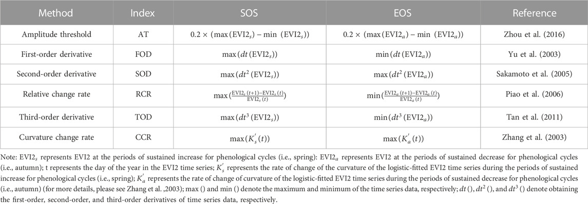
TABLE 1. Description of the six algorithms for extracting the start-of-season (SOS) and end-of-season (EOS) from the EVI2 time series.

We used the Savitzky–Golay (S-G) method (Savitzky and Golay, 1964) to remove the outliers of the EVI2 time series and interpolated the eight-day EVI2 time series to one-day intervals. We divided the EVI2 time series of a growing season into a growth period and a dormancy period and used Eq. 2 to fit them.

$y\left(t\right)=\frac{c}{1+e^{a+bt}}+d,(2)$

where t denotes the day of the year, $\mathrm{y}\left(\mathrm{t}\right)$ denotes the EVI2 value on date t, and a, b, c, and d are fitting parameters. We used this data series when fitting the EVI2 of vegetation dormancy with Eq. 2.

2.2 Test region

We selected the conterminous United States as the test region; it has a rich distribution of vegetation types, such as a large number of deciduous broadleaf forests distributed in its east and west, and vast grassland, shrub, and some deciduous broadleaf forests distributed in its center. In addition, many digital camera observation stations for tracking vegetation phenology have been established in the conterminous United States, and data from these stations can be used to evaluate the performance of vegetation phenology extracted from satellite remote sensing data using phenoC++.

2.3 MODIS data

The MODIS/Terra surface reflectance eight-day 250-m product (MOD09Q1, Version 6) (Vermote et al., 2015) was used to retrieve the vegetation phenology in the developed open-source tool. MOD09Q1 includes two surface reflectance bands (red band, 620–670 nm; near-infrared band, 841–876 nm) with eight-day temporal resolution and an approximately 250-m spatial resolution. The MODIS/Terra and Aqua Land Cover Dynamics Yearly L3 Global 500 m SIN Grid (MCD12Q2, Version 6), which provides vegetation phenology over global land surfaces (Friedl et al., 2019), was used as reference data for evaluating the performance of the developed open-source tool. Both MOD09Q1 and MCD12Q2 are available from https://search.earthdata.nasa.gov/. We used the greenup layer (i.e., SOS) and the dormancy layer (i.e., EOS) of MCD12Q2 for analysis. In the MCD12Q2 product, SOS and the EOS would be obtained when EVI2 crosses 15% of the segment EVI2 amplitude for the first or last time, respectively.

2.4 PhenoCam data

We used PhenoCam Dataset v2.0 (Seyednasrollah et al., 2019) as validation data for evaluating the performance of vegetation phenophases extracted from the MOD09Q1 EVI2 time series by phenoC++. The PhenoCam sites were established in 2008 and use networked digital cameras to track vegetation phenology. There are 500 sites, particularly located in North America. The PhenoCam Dataset v2.0 (Seyednasrollah et al., 2019) can be obtained from https://phenocam.sr.unh.edu/webcam/. We used the phenology records of 28 deciduous broadleaf forest (DBF) sites, 43 shrubland (SHR) sites, and 38 grassland (GRA) sites from 2009 to 2018 for satellite-retrieved phenology validation (as shown in Figure 1). In the PhenoCam Dataset, three threshold values (i.e., 10%, 25%, and 50%) of the green chromatic coordinate index mean (G_cc-mean) were employed to retrieve vegetation phenophases. Among them, the threshold value of 50% of the vegetation index time series is rarely used to retrieve vegetation phenophases from remote sensing data, while the SOS and EOS retrieved by threshold values of 10% and 25% of the vegetation index time series are similar (Ruan et al., 2021). Therefore, SOS and EOS of the PhenoCam Dataset v2.0, which were retrieved from the threshold values of 25% of G_cc-mean amplitude, were selected for validation.

FIGURE 1

FIGURE 1. Test region and locations of selected PhenoCam sites, including deciduous broadleaf forest (DBF), shrubland (SHR), and grassland (GRA).

3 Results

3.1 Performance of phenoC++ on a site scale

After obtaining the EVI2 time series from MOD09Q1, we used phenoC++ with the six methods to retrieve the vegetation phenology from 2009 to 2018 and evaluated the retrieved vegetation phenology using PhenoCam-observed phenology. Pearson correlation coefficient and root-mean-square error (RMSE) were used to evaluate the performance of vegetation phenology retrieved by the open-source tool. Figure 2 shows the scatterplots for the regression result between the PhenoCam-observed SOS and the satellite-retrieved SOS using multiple methods. In Figure 2, most points are around 1: 1, demonstrating that SOS derived from two independent datasets is consistent. Compared with PhenoCam-observed SOS, the SOS derived from MOD09Q1 EVI2 by phenoC++ with six methods obtained r-values of 0.75, 0.76, 0.75, 0.76, 0.64, and 0.67, and RMSE values of 21.36, 20.41, 22.38, 19.11, 33.56, and 32.14, respectively. The TOD method produced the worst SOS, while the other methods performed similarly to each other.

FIGURE 2

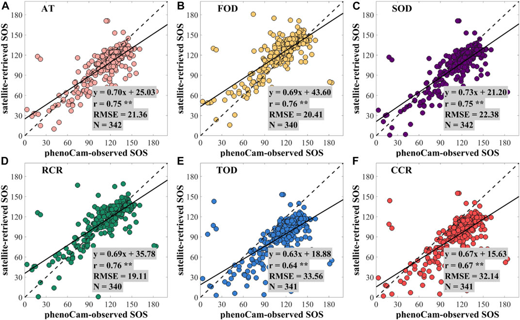
FIGURE 2. Scatterplots for the regression analysis between the PhenoCam-observed SOS and the satellite-retrieved SOS using the methods of (A) amplitude threshold (AT), (B) first-order derivative (FOD), (C) second-order derivative (SOD), (D) relative change rate (RCR), (E) third-order derivative (TOD), and (F) curvature change rate (CCR). ** denotes a p-value of two-tailed Student's t-tests of <0.01. N denotes the number of PhenoCam observation sites.

Figure 3 shows the scatterplots for the regression analysis between the PhenoCam-observed EOS and the satellite-retrieved EOS using phenoC++ with six methods. Most points in Figure 3 are also around 1: 1, but they are more discrete than the SOS scatter points, as shown in Figure 2. Compared with PhenoCam-observed EOS, the EOS derived from MOD09Q1 EVI2 by phenoC++ with six methods obtained r-values of 0.58, 0.59, 0.57, 0.56, 0.36, and 0.40, and RMSE values of 52.43, 46.68, 55.13, 49.46, 71.13, and 69.34, respectively. The CCR method obtained the worst EOS, and the other methods had similar performance to each other. Figures 2 and 3 show that, compared with PhenoCam-observed phenology, the accuracy of satellite-retrieved SOS is slightly higher than that of satellite-retrieved EOS, which is consistent with previous results reported by Li et al. (2019). This may be caused by the different sensitivities of G_cc and EVI2 for detecting vegetation growth changes. During vegetation growth, G_cc and EVI2 both rapidly increase. EVI2 decreases slightly during vegetation dormancy, but G_cc rapidly decreases if leaf color changes.

FIGURE 3

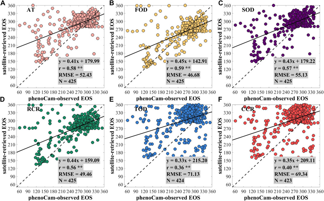
FIGURE 3. Scatterplots for the regression analysis between the PhenoCam-observed EOS and the satellite-retrieved EOS using the methods of (A) amplitude threshold (AT), (B) first-order derivative (FOD), (C) second-order derivative (SOD), (D) relative change rate (RCR), (E) third-order derivative (TOD), and (F) curvature change rate (CCR). ** denotes a p-value of two-tailed Student's t-tests of <0.01. N denotes the number of PhenoCam observation sites.

Figure 4 illustrates the regression analysis of SOS/EOS obtained from MCD12Q2 and the PhenoCam Dataset. We used it to indirectly evaluate the performance of phenoC++. The regression analysis indicated that the SOS of MCD12Q2 achieved an r-value of 0.45 and an RMSE value of 25.22, and the EOS of MCD12Q2 achieved an r-value of 0.64 and an RMSE value of 50.67. Comparison with the PhenoCam Dataset found that the SOS of MCD12Q2 is unfavorable with the SOS retrieved by the phenoC++. The least desirable method of phenoC++ (TOD) obtained an r-value of 0.64, and its performance shows that it is better than the MCD12Q2 SOS, with an r-value of 0.45. For EOS, that of MCD12Q2 (r = 0.64; RMSE = 50.67) is better than the EOS obtained by phenoC++. Nevertheless, the SOS/EOS for retrieval by phenoC++ (N ≈ 420) obtained more effective pixels in the PhenoCam observation sites than MCD12Q2 (N = 288). Through the regression analyses between the phenoC++-retrieved phenology/MCD12Q2 with PhenoCam-observed phenology, we found an RMSE range of about 20–55 days. This is similar to the results of Xin, et al. [42], who used satellite-retrieved phenology for comparison with US National Phenology Network data (RMSE ∼25–55 days), and Li, et al. [43], who used 30 m fine-resolution satellite-retrieved phenology to compare PhenoCam-observed phenology (RMSE about 25 days; r of SOS is 0.66 and r of EOS is 0.43). The main reason for the large RMSE could be that the observation scale between the satellite and PhenoCam is inconsistent, and the observation of spectral difference between the satellite sensor and PhenoCam-camera.

FIGURE 4

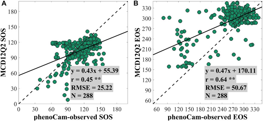
FIGURE 4. Scatterplots for the regression analysis between the PhenoCam-observed SOS/EOS and the SOS/EOS of MCD12Q2 at (A) the start of season (SOS) and (B) the end of season (EOS). ** denotes a p-value of two-tailed Student's t-tests of <0.01. N denotes the number of PhenoCam observation sites.

Figure 5 shows the profile of phenophases obtained from MOD09Q1 by phenoC++ with six methods and MCD12Q2. The average SOS estimated by the six methods and the AT and SOD methods were similar to the MCD12Q2 SOS. Compared with the MCD12Q2 SOS, the FOD and RCR methods were overestimated, while the TOD and CCR methods were underestimated. Meanwhile, the average EOS estimated by the six methods and the AT and SOD methods were similar to the MCD12Q2 EOS. Compared with the MCD12Q2 EOS, the TOD and CCR methods were overestimated, while the FOD and RCR methods were underestimated. Overall, the phenophases (SOS and EOS) estimated by phenoC++ were in line with those of MCD12Q2 with reliable performance.

FIGURE 5

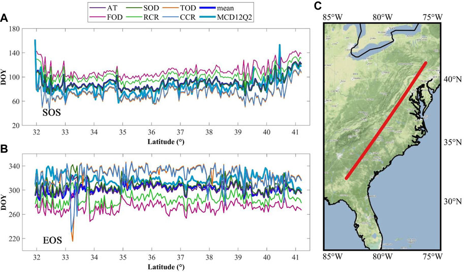
FIGURE 5. Profile of the start of season (SOS) and the end of season (EOS) in 2017 derived from two different data sources. (A) Profile of SOS; (B) profile of EOS; (C) location of the profile. The average value of phenophases was calculated every 0.05° along the profile. MCD12Q2 denotes the phenophases obtained from the MCD12Q2 product; AT, FOD, SOD, RCR, TOD, and CCR denote the phenophases estimated from the MOD09Q1 EVI2 time series using corresponding methods, and “mean” denotes the average value of the phenophases estimated from the fused EVI2 time series by six methods.

3.2 The performance of phenoC++ on a regional scale

Figure 6 shows the spatial distribution for SOS over the conterminous United States, including the MCD12Q2 SOS and the SOS obtained from the MOD09Q1 EVI2 time series by phenoC++ with six methods. The SOS values obtained from MOD09Q1 EVI2 (Figures 6B–G) are close to MCD12Q2 SOS (Figure 6A) on a regional scale, while the former SOS is generally slightly earlier than the latter SOS in the southwest of the USA and slightly more delayed than the latter SOS in the northeast. Compared with Figure 6A, the SOS retrieved by phenoC++ shows high-value (red) pixels in North Dakota, South Dakota, Minnesota, Iowa, Illinois, Indiana, Ohio, and Pennsylvania, especially in the results from the FOD and RCR methods. From Figures 6A–G, the SOS in the southwest of the USA (less than 80 days) is earlier than in the northeast of the USA (more than 80 days, mostly more than 140 days). This shows that the vegetation season begins earlier in the southwest of the USA than that in the northeast. In addition, the MCD12Q2 SOS (Figure 6A) shows more data gaps in the southwest of the USA, which is not shown in the SOS retrieved by phenoC++. This phenomenon could be caused by the MOCD12Q2 algorithm’s inability to effectively retrieve phenological dates from remote sensing data in places with relatively sparse vegetation.

FIGURE 6

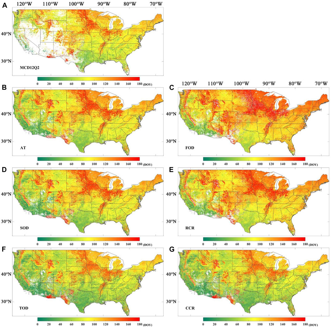
FIGURE 6. Spatial distribution for the start of season (SOS) in 2017. (A) SOS obtained from MCD12Q2; (B) SOS derived from MOD09Q1 EVI2 time series by amplitude threshold (AT); (C) SOS derived from MOD09Q1 EVI2 time series by first-order derivative (FOD); (D) SOS derived from MOD09Q1 EVI2 time series by second-order derivative (SOD); (E) SOS derived from MOD09Q1 EVI2 time series by relative change rate (RCR); (F) SOS derived from MOD09Q1 EVI2 time series by third-order derivative (TOD); (G) SOS derived from MOD09Q1 EVI2 time series by curvature change rate (CCR).

Figure 7 shows the spatial distribution of the EOS over the conterminous United States, including the MCD12Q2 EOS and the EOS obtained from the MOD09Q1 EVI2 time series with phenoC++ with six methods. The EOS values obtained from MOD09Q1 EVI2 (Figures 7B–G) are close to MCD12Q2 EOS (Figure 7A) on the regional scale, especially in Figures 7B and 7D. The EOS obtained from MOD09Q1 EVI2 with the FOD (Figure 7C) and RCR (Figure 7E) methods are slightly earlier than the EOS of MCD12Q2, and the EOS obtained from MOD09Q1 EVI2 with the TOD (Figure 7F) and CCR (Figure 7G) methods are generally slightly delayed than the EOS of MCD12Q2. From Figures 7A–G, the EOS in the northwest of the USA (about 240 days) is earlier than that in the southeast (more than 300 days, mostly more than 320 days). This suggests that the vegetation season ends later in the southeast of the USA than that in the northwest. In addition, like Figure 6A, Figure 7A also has data gaps in the southwest of the USA.

FIGURE 7

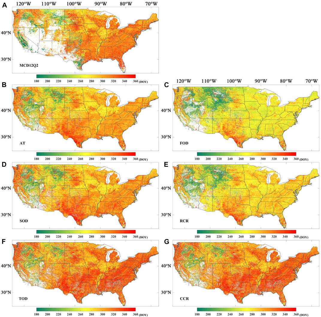
FIGURE 7. Spatial distribution for the end of season (EOS) in 2017. (A) EOS obtained from MCD12Q2; (B) EOS derived from MOD09Q1 EVI2 time series by amplitude threshold (AT); (C) EOS derived from MOD09Q1 EVI2 time series by first-order derivative (FOD); (D) EOS derived from MOD09Q1 EVI2 time series by second-order derivative (SOD); (E) EOS derived from MOD09Q1 EVI2 time series by relative change rate (RCR); (F) EOS derived from MOD09Q1 EVI2 time series by third-order derivative (TOD); (G) EOS derived from MOD09Q1 EVI2 time series by curvature change rate (CCR).

4 Discussion

Previous research has provided phenology-retrieval tools, such as in the R package (Hufkens et al., 2018; Kong et al., 2022) and the MATLAB platform (Jönsson and Eklundh, 2004). However, their stability and speed in large-scale vegetation phenology retrieval are not as effective as programs written in C++. This study provides a C++ compiled running program (phenoC++), which is compiled under the Linux system. If users need to run it under Windows, they must install the C++ and GDAL environments before compiling it. phenoC++ only retrieves two commonly used and critical phenology metrics (i.e., SOS and EOS). If users need to retrieve other phenology metrics or add more algorithms, the source code of phenoC++ can be modified.

We compared the performance of TIMESAT software for retrieving the phenology metrics to that of phenoC++. Areas of 802 × 642 pixels and 5164 × 4193 pixels (about the area of Texas) from MOD09Q1 were used to test the performance of TIMESAT software and phenoC++. The test computer was configured as follows. The computer system was Ubuntu 16.04, and the CPU model was Intel(R) Xeon(R) Platinum 8269CY CPU @ 2.50 GHz (52 threads) with 512 GB of computer memory. After data preprocessing, TIMESAT ran for approximately 2.5 min in the 802 × 642-pixel region, occupying 0.2 GB of memory, while in the 5164 × 4193-pixel test, the running time was approximately 25 min and the memory occupied 0.4 GB. After data preprocessing, the phenoC++ test in the 802 × 642-pixel region took approximately 0.63 min and used 0.2 GB of memory, while the test for 5164 × 4193 pixels took approximately 24.5 min and used 4.8 GB of memory. This shows that the running speeds of the TIMESAT and phenoC++ are similar and that phenoC++ occupies more memory when the same number of CPU threads are used. This is because TIMESAT uses multiple steps to retrieve vegetation phenology, whereas phenoC++ is integrated, which is more user-friendly. Compared with TIMESAT, phenoC++ also has the following advantages. 1) phenoC++ outputs six algorithms’ results for SOS or EOS, while TIMESAT only outputs threshold method results for SOS and EOS. 2) phenoC++ outputs phenology metrics in GeoTIFF format images with geographical coordinates, which are more convenient for use with other geospatial data, while TIMESAT outputs binary files. 3) The code of phenoC++ is open source, while TIMESAT is not. In addition, we also tested phenoC++ for retrieving vegetation phenology from MOD09Q1 EVI2 with 250-m spatial resolution over the USA (22,731 × 9774 pixels). The run time of phenoC++ was approximately 4.5 h, and the memory occupied was approximately 57.9 GB. Therefore, phenoC++ is an efficient and easy-to-use software tool.

5 Conclusion

Vegetation phenology is a first-order control on ecosystem productivity, so its accurate and rapid retrieval from satellite remote sensing data is key to understanding the feedback between the climate and the biosphere. We developed phenoC++, a tool that uses parallel C++ technology to retrieve start-of-season (SOS) and end-of-season (EOS) vegetation data from satellite time series data. Compared to traditional tools, the innovative features of phenoC++ include 1) integrating six algorithms for retrieving SOS and EOS; 2) rapid large-scale data processing with simple input startup parameters; 3) outputting phenology metrics as GeoTIFF format images, which are more convenient to use with other geospatial data.

We implemented phenoC++ to quickly and easily obtain the spatial distribution of SOS and EOS at 250-m spatial resolution over the conterminous United States using MODIS time-series data. We then evaluated phenoC++ performance for retrieving SOS and EOS on a site scale using PhenoCam Dataset v2.0. The results show that SOS derived from MODIS images by phenoC++ with six methods obtained r-values of 0.75, 0.76, 0.75, 0.76, 0.64, and 0.67, and RMSE values of 21.36, 20.41, 22.38, 19.11, 33.56, and 32.14, respectively. The satellite-retrieved EOS by phenoC++ with six methods obtained r-values of 0.58, 0.59, 0.57, 0.56, 0.36, and 0.40, respectively, and RMSE values of 52.43, 46.68, 55.13, 49.46, 71.13, and 69.34, respectively. Using PhenoCam-observed phenology as a baseline, SOS retrieved by phenoC++ outperforms MCD12Q2 SOS, while EOS retrieved by phenoC++ is slightly inferior to that of MCD12Q2 EOS. Moreover, compared to MCD12Q2, phenoC++-retrieved vegetation phenology yielded more effective pixels on a regional scale.

phenoC++ can rapidly produce robust vegetation phenology on a large scale. The SOS and EOS spatial distribution information on vegetation is more easily accessible through phenoC++, which will help solve large-scale ecological phenology problems.

Data availability statement

The original contributions presented in the study are included in the article/supplementary materials, further inquiries can be directed to the corresponding author.

Author contributions

YR and BR conceived and designed phenoC++ with contributions from QX and XZ. YR developed the application programming by parallel C++; BR analyzed the data and interpreted the results. YR drafted the manuscript. All authors commented on and approved the final manuscript.

Funding

The Project Supported by the Open Fund of Key Laboratory of Urban Land Resources Monitoring and Simulation, Ministry of Natural Resources, Guangzhou Science and Technology project (grant no. 2023A04J1541), and the National Natural Science Foundation of China (grant no. 42071441).

Acknowledgments

The authors thank the editor and reviewers for their constructive comments.

Conflict of interest

The authors declare that the research was conducted in the absence of any commercial or financial relationships that could be construed as a potential conflict of interest.

Publisher’s note

All claims expressed in this article are solely those of the authors and do not necessarily represent those of their affiliated organizations, or those of the publisher, the editors, and the reviewers. Any product that may be evaluated in this article, or claim that may be made by its manufacturer, is not guaranteed or endorsed by the publisher.

References

Ao, Z., Sun, Y., and Xin, Q. (2020). Constructing 10-m NDVI time series from landsat 8 and sentinel 2 images using convolutional neural networks. IEEE Geoscience Remote Sens. Lett. 18, 1461–1465. doi:10.1109/lgrs.2020.3003322

CrossRef Full Text | Google Scholar

Bolton, D. K., Gray, J. M., Melaas, E. K., Moon, M., Eklundh, L., and Friedl, M. A. (2020). Continental-scale land surface phenology from harmonized Landsat 8 and Sentinel-2 imagery. Remote Sens. Environ. 240, 111685. doi:10.1016/j.rse.2020.111685

CrossRef Full Text | Google Scholar

Caparros-Santiago, J. A., Rodriguez-Galiano, V., and Dash, J. (2021). Land surface phenology as indicator of global terrestrial ecosystem dynamics: A systematic review. Isprs J. Photogrammetry Remote Sens. 171, 330–347. doi:10.1016/j.isprsjprs.2020.11.019

CrossRef Full Text | Google Scholar

De Beurs, K. M., and Henebry, G. M. (2008). Northern annular mode effects on the land surface phenologies of northern eurasia. J. Clim. 21 (17), 4257–4279. doi:10.1175/2008jcli2074.1

CrossRef Full Text | Google Scholar

Defries, R. S., Field, C. B., Fung, I., Justice, C. O., Los, S., Matson, P. A., et al. (1995). Mapping the land surface for global atmosphere-biosphere models: Toward continuous distributions of vegetation's functional properties. J. Geophys. Res. Atmos. 100 (D10), 20867–20882. doi:10.1029/95jd01536

CrossRef Full Text | Google Scholar

Elmore, A. J., Guinn, S. M., Minsley, B. J., and Richardson, A. D. (2012). Landscape controls on the timing of spring, autumn, and growing season length in mid-Atlantic forests. Glob. Change Biol. 18 (2), 656–674. doi:10.1111/j.1365-2486.2011.02521.x

CrossRef Full Text | Google Scholar

Elmore, A. J., Nelson, D., Guinn, S. M., and Paulman, R. (2017). Landsat-based phenology and tree ring characterization. East. U. S. For., 1984–2013.

Google Scholar

Foley, J. A., Prentice, I. C., Ramankutty, N., Levis, S., Pollard, D., Sitch, S., et al. (1996). An integrated biosphere model of land surface processes, terrestrial carbon balance, and vegetation dynamics. Glob. Biogeochem. Cycles 10 (4), 603–628. doi:10.1029/96gb02692

CrossRef Full Text | Google Scholar

Friedl, M., Gray, J., and Sulla-Menashe, D. (2019). Land surface phenology from MODIS: Characterization of the Collection 5 global land cover dynamics product. Remote Sens. Environ. 114 (8), 1805–1816. doi:10.1016/j.rse.2010.04.005

CrossRef Full Text | Google Scholar

Gao, X., Gray, J. M., and Reich, B. J. (2021). Long-term, medium spatial resolution annual land surface phenology with a Bayesian hierarchical model. Remote Sens. Environ. 261, 112484. doi:10.1016/j.rse.2021.112484

CrossRef Full Text | Google Scholar

Hufkens, K., Basler, D., Milliman, T., Melaas, E. K., and Richardson, A. D. (2018). An integrated phenology modelling framework in r. Methods Ecol. Evol. 9 (5), 1276–1285. doi:10.1111/2041-210x.12970

CrossRef Full Text | Google Scholar

Jönsson, P., and Eklundh, L. (2004). TIMESAT—A program for analyzing time-series of satellite sensor data. Comput. Geosciences 30 (8), 833–845. doi:10.1016/j.cageo.2004.05.006

CrossRef Full Text | Google Scholar

Kollert, A., Bremer, M., Löw, M., and Rutzinger, M. (2021). Exploring the potential of land surface phenology and seasonal cloud free composites of one year of Sentinel-2 imagery for tree species mapping in a mountainous region. Int. J. Appl. Earth Observation Geoinformation 94, 102208. doi:10.1016/j.jag.2020.102208

CrossRef Full Text | Google Scholar

Kong, D., Mcvicar, T. R., Xiao, M., Zhang, Y., Peña-Arancibia, J. L., Filippa, G., et al. (2022). phenofit: An R package for extracting vegetation phenology from time series remote sensing. Methods Ecol. Evol. 13 (7), 1508–1527. doi:10.1111/2041-210x.13870

CrossRef Full Text | Google Scholar

Li, X., Zhou, Y., Meng, L., Asrar, G. R., Lu, C., and Wu, Q. (2019). A dataset of 30 m annual vegetation phenology indicators (1985–2015) in urban areas of the conterminous United States. Earth Syst. Sci. Data 11 (2), 881–894. doi:10.5194/essd-11-881-2019

CrossRef Full Text | Google Scholar

Menzel, A. (2002). Phenology: Its importance to the global change community. Clim. Change 54 (4), 379–385. doi:10.1023/a:1016125215496

CrossRef Full Text | Google Scholar

ORNL Distributed Active Archive Center, Fischer A (1994). A model for the seasonal variations of vegetation indices in coarse resolution data and its inversion to extract crop parameters. Remote Sens. Environ. 48 (2), 220–230. doi:10.1016/0034-4257(94)90143-0

CrossRef Full Text | Google Scholar

Peng, D., Wang, Y., Xian, G., Huete, A. R., Huang, W., Shen, M., et al. (2021). Investigation of land surface phenology detections in shrublands using multiple scale satellite data. Remote Sens. Environ. 252, 112133. doi:10.1016/j.rse.2020.112133

CrossRef Full Text | Google Scholar

Peng, D., Zhang, X., Wu, C., Huang, W., Gonsamo, A., Huete, A. R., et al. (2017). Intercomparison and evaluation of spring phenology products using National Phenology Network and AmeriFlux observations in the contiguous United States. Agric. For. Meteorology 242, 33–46. doi:10.1016/j.agrformet.2017.04.009

CrossRef Full Text | Google Scholar

Piao, S., Fang, J., Zhou, L., Ciais, P., and Zhu, B. (2006). Variations in satellite-derived phenology in China's temperate vegetation. Glob. Change Biol. 12 (4), 672–685. doi:10.1111/j.1365-2486.2006.01123.x

CrossRef Full Text | Google Scholar

Richardson, A. D., Hufkens, K., Milliman, T., Aubrecht, D. M., Chen, M., Gray, J. M., et al. (2018). Tracking vegetation phenology across diverse North American biomes using PhenoCam imagery. Sci. Data 5 (1), 180028. doi:10.1038/sdata.2018.28

PubMed Abstract | CrossRef Full Text | Google Scholar

Ruan, Y., Zhang, X., Xin, Q., Sun, Y., Ao, Z., and Jiang, X. (2021). A method for quality management of vegetation phenophases derived from satellite remote sensing data. Int. J. Remote Sens. 42 (15), 5811–5830. doi:10.1080/01431161.2021.1931534

CrossRef Full Text | Google Scholar

Sakamoto, T., Yokozawa, M., Toritani, H., Shibayama, M., Ishitsuka, N., and Ohno, H. (2005). A crop phenology detection method using time-series MODIS data. Remote Sens. Environ. 96 (3), 366–374. doi:10.1016/j.rse.2005.03.008

CrossRef Full Text | Google Scholar

Savitzky, A., and Golay, M. J. E. (1964). Smoothing and differentiation of data by simplified least squares procedures. Anal. Chem. 36 (8), 1627–1639. doi:10.1021/ac60214a047

CrossRef Full Text | Google Scholar

Seyednasrollah, B., Young, A. M., Hufkens, K., Milliman, T., Friedl, M. A., Frolking, S., et al. (2019). PhenoCam Dataset v2.0: Vegetation Phenology from Digital Camera Imagery, 2000-2018. Oak Ridge, TN, United States: ORNL DAAC. doi:10.3334/ORNLDAAC/1674

CrossRef Full Text | Google Scholar

Tan, B., Morisette, J. T., Wolfe, R. E., Gao, F., Ederer, G. A., Nightingale, J., et al. (2011). An enhanced TIMESAT algorithm for estimating vegetation phenology metrics from MODIS data. IEEE J. Sel. Top. Appl. Earth Observations Remote Sens. 4 (2), 361–371. doi:10.1109/jstars.2010.2075916

CrossRef Full Text | Google Scholar

Templ, B., Koch, E., Bolmgren, K., Ungersböck, M., Paul, A., Scheifinger, H., et al. (2018). Pan European phenological database (PEP725): A single point of access for European data. Int. J. Biometeorology 62 (6), 1109–1113. doi:10.1007/s00484-018-1512-8

PubMed Abstract | CrossRef Full Text | Google Scholar

Vermote, E., Walker, J. J., De Beurs, K. M., Wynne, R. H., and Gao, F. (2015). MOD09Q1 MODIS/Terra Surface Reflectance 8-Day L3 Global 250m SIN Grid V006. NASA EOSDIS Land Processes DAAC, 117, 381–393.Evaluation of Landsat and MODIS data fusion products for analysis of dryland forest phenologyRemote Sens. Environ.

Google Scholar

Yu, F., Price, K. P., Ellis, J., and Shi, P. (2003). Response of seasonal vegetation development to climatic variations in eastern central Asia. Remote Sens. Environ. 87 (1), 42–54. doi:10.1016/s0034-4257(03)00144-5

CrossRef Full Text | Google Scholar

Zhang, X., Friedl, M. A., Schaaf, C. B., Strahler, A. H., Hodges, J. C. F., Gao, F., et al. (2003). Monitoring vegetation phenology using MODIS. Remote Sens. Environ. 84 (3), 471–475. doi:10.1016/s0034-4257(02)00135-9

CrossRef Full Text | Google Scholar

Zhang, X., Liu, L., Liu, Y., Jayavelu, S., Wang, J., Moon, M., et al. (2018). Generation and evaluation of the VIIRS land surface phenology product. Remote Sens. Environ. 216, 212–229. doi:10.1016/j.rse.2018.06.047

CrossRef Full Text | Google Scholar

Zhang, X., Wang, J., Henebry, G. M., and Gao, F. (2020). Development and evaluation of a new algorithm for detecting 30 m land surface phenology from VIIRS and HLS time series. Isprs J. Photogrammetry Remote Sens. 161, 37–51. doi:10.1016/j.isprsjprs.2020.01.012

CrossRef Full Text | Google Scholar

Zhou, D., Zhao, S., Zhang, L., and Liu, S. (2016). Remotely sensed assessment of urbanization effects on vegetation phenology in China's 32 major cities. Remote Sens. Environ. 176, 272–281. doi:10.1016/j.rse.2016.02.010

CrossRef Full Text | Google Scholar