Low-activity hotspot investigation method via scanning using deep learning

Small areas of elevated activity are a concern during a final status scan survey of residual radioactivity of decommissioned and contaminated sites. Due to the characteristics of scanning, the lower limit of detection is relatively high because the number of counts is low due to the short measurement time. To overcome this, an algorithm capable of finding hotspots with little information through deep learning was developed. The developed model using an artificial neural network was trained with the scan survey data acquired from a Monte Carlo-based computational simulation. A random mixing method was used to obtain sufficient training data. In order to respond properly to the experimental data, training and verification were conducted in various situations, in this case, in the presence or absence of random background counts and collimators and various source concentrations. Experimental data were obtained using a conventional detector, in this case, the 3″ × 3″ NaI(Tl). The advantages and limitations to the proposed method are as follows. Results were well predicted even in cases at less than 1 Bq/g, which is lower than the scanned minimum detectable concentration (MDC) of the detection system. It is a great advantage that it can detect contaminated areas that are lower than the existing scan’s minimum detectable concentration. However, the limitation is that it cannot be predicted, and the accuracy is low in multi-sourced scans. The source position and size are also important in residual radioactive evaluations, and scanning data images were evaluated in artificial neural network modes with suitable prediction results. The proposed methodology proved the high accuracy of hotspot prediction for low-activity sites and showed that this technology can be used as an efficient and economical hotspot scanning technology and can be extended to an automated system.

1 Introduction

Radiation measurements at decommissioned sites or in a post-accident environment are very important for radiation protection (Abu-Eid et al., 2012; Huang et al., 2013; Lee et al., 2010; Takahashi et al., 2015). After decontamination, such sites are investigated to confirm that the activity concentration is lower than the release criteria. Laboratory sample preparation is an important step, but it is an expensive and time-consuming step during measurements of elevated radioactivity levels. However, because it is not possible to accurately measure all sites in a wide area, a dynamic survey method or scanning has been used (Hong et al., 2014).

The derived concentration guideline level (DCGL) is the residual radioactivity that can be distinguished from the background level, and it is assumed that the contamination source is uniformly distributed in the contaminated area of the site. The average value of the residual radioactivity for each region of interest should not exceed the DCGL value for each nuclide. In areas with locally high residual radioactivity (hotspots), the number and locations of measurements are determined using the DCGL_EMC method of calculating the derived concentration standard. Also, DCGL_EMC is a value applied to an area with high local residual radioactivity, and it is the site release standard for hotspot areas. In addition, the actual MDC of the selected scanning technique is compared to the required scan MDC. If the actual scan MDC is smaller than the required scan MDC, the selected scanning technique is considered to have adequate sensitivity for hotspot measurements. In residual contamination level surveys of large-scale sites, the scan MDC is derived according to the appropriate measurement conditions (e.g., scan speed, detector type, etc.) to evaluate hotspots quickly and accurately, and an investigation plan is established (United States Nuclear Regulatory Commission, 2005).

Measurements of hotspots at the site are performed through a dynamic survey (scan survey) because the scan MDC value changes depending on the type of the detector, survey speed, and height of the detector. Therefore, it is necessary to establish proper measurement conditions according to the release criteria (Kurtz, 2017; Abelquist et al., 2020; Owens et al., 2018; Hong et al., 2011). Unlike a static survey, for a scan survey, the target area is measured during the continuous movement of the detector, and the measurement time within the target area is short. Therefore, the minimum detectable concentration (MDC) of the scan survey is relatively high. It is possible to increase the measurement time to meet the desired concentration, but if it exceeds a certain time limit, the advantage of the scan survey for quick measurements will be lost. The scan survey method is generally used to evaluate the distribution of contamination at sites in the final status survey (FSS) (Abelquist, 2013; Lee et al., 2020). Also, the scan MDC varies depending on the survey conditions and the type of the instrument used. In 2016–2019, a study to evaluate scan MDC outcomes for ¹³⁷Cs with high soil adsorption levels was conducted (Kim et al., 2020). This study evaluated the sensitivity, according to the dynamic irradiation conditions, by changing the scan speed and measuring the height using 2″ NaI(Tl) and 3″ NaI(Tl) crystals. Recently, various scenarios have been investigated for uranium enrichment facilities in Spain using scan measurement methods (Vico et al., 2021). These studies follow the multi-agency radiation survey and site investigation Manual (MARSSIM) assessment method, which is the methodology followed in many countries to demonstrate compliance with radiation standards. According to previous studies, it was found that the higher the scan speed and the lower the efficiency of the instrument were, the higher the contamination range became. For this reason, it is necessary to develop a method capable of investigating hotspots with a fast scan rate.

The gamma camera was a representative technology for investigation of hotspots (Gal et al., 2006; Okada et al., 2014). However, these devices have a low sensitivity of a few hundreds of μGy/h because they lose too many gamma ray signals as they utilize a pinhole collimator. Therefore, the gamma camera has been used for high levels of contamination, such as inspections of nuclear power plants, radioisotope generators, and nuclear accident sites. The Compton camera has been used for low-dose rate levels and for relatively accurate source position tracking (Suzuki et al., 2013). Compared to a gamma camera, this camera can be used at relatively low doses and can locate sources at the level of hundreds of nGy/h. Based on this, a compactly manufactured Compton camera feasible for use at sites after an accident was developed (Sato et al., 2020; Sato et al., 2018). A gamma ray detector was attached to an unmanned aerial vehicle which flew over the scanning area, whereas the conventional Compton camera used a pixelated gamma ray detector. The conventional type incurs a high cost because it needs two pixelated photon detectors. However, in a study involving the compact Compton camera, the Compton cone was calculated using data acquired when moving along the flight route. Therefore, this type did not require multiple detectors, which reduces its weight and cost. However, a problem arose when multiple sources were positioned adjacently as distance correction among the Compton cones was difficult and the process only indicated whether there was any source in the area. Device-oriented studies, such as those that automate a conventional detector by loading it into a vehicle, have also been carried out (Lee et al., 2020; Ardiny et al., 2019), but there are only a few software-based approaches.

Artificial neural networks have been widely applied in various fields in engineering to solve complex multi-variable problems (Shafiq et al., 2021a, Shafiq et al., 2021b, Shafiq et al., 2022; Colak et al., 2022), improve the accuracy of classification of image-like data (Sibille et al., 2019), and spectroscopy (Galib et al., 2021; Cui et al., 2019; Li et al., 2021). By training the neural network model, also called deep learning, meaningful results can be obtained from the data at a level that is difficult for humans to find or is statistically insignificant due to lack of information. By using deep learning, radionuclides can be identified from a full-energy peak that is unshaped due to lack of counts and from a spectrum acquired with poor energy resolution, such as that by a plastic scintillator (Daniel et al., 2020; Jeon et al., 2020).

Based on these outcomes, in this study, a low-level hotspot investigation method based on an ANN-based deep-learning algorithm and scanning data imagery is proposed. The method is based on deep learning and determines hotspots in the scanning area with activity levels lower than those of the conventional scan MDC. In the application of deep learning on gamma ray spectroscopy, although the number of counts was not sufficient in the range of interest, the presence of a certain radionuclide can be determined using the data from other channels. Taking this into consideration, if the scanned data are imaged, each pixel becomes a data channel adjacent to the others, and even if the amount of data obtained directly above the hotspot are small, the location and size of the hotspot can be predicted using the surrounding data. The present study uses scanning data imagery and undertakes training of the ANN model using computational simulation data and verification of hotspot prediction results through both simulations and experiments.

2 Materials and methods

The purpose of the deep learning-based hotspot investigation algorithm proposed in this study is supporting to identify radioactively elevated hotspots using a deep learning model trained with simulation data. This section describes how the neural network model is configured and the training data are prepared.

2.1 Hotspot investigation algorithm with an ANN

The ANN model works similarly to how neurons in the brain work (Kim et al., 2019). Neurons (nodes) between layers are connected with weights. The values in the input layer are multiplied by weights through the hidden layer, and the result is obtained at the output layer. The errors between the answers and results are reduced by updating the weights with an optimization function and a loss function. By repeating this with a proper number of cycles, the model can predict the desired target value.

Figure 1 shows a conceptual diagram of the hotspot investigation algorithm with deep learning. An ANN model is trained using image-like count rate scanning data obtained from scanning simulation. In this study, the input data have a shape of 24 × 24. Each pixel contains the count rate in a scanning interval. Candidates for neural network models include fully connected sequential neural networks, convolutional neural networks, and recurrent neural networks. Convolutional neural networks are widely used in 2D data such as images and are useful for extracting features by training the correlation between adjacent pixels. It is particularly effective for problems that are too expensive to train with a fully connected neural network when the number of pixels in the image is large. However, in this study, the number of pixels is small because the scanning range is not large at one time. There are also cases where the hotspot covers only one pixel because the area per scanning interval is large. Therefore, the convolutional neural network is excluded because it may be disadvantageous in learning sparse image data. Recurrent neural networks are used to learn sequential data such as spectra or waveforms. If the spectroscopy data from the scintillator detector are directly used to train the model, it would be very useful, but in this study, the counting rate data were used. Therefore, the recurrent neural network is also excluded. As a result, this study does not consider other models because the computational cost is not large even when using a fully connected sequential neural network.

FIGURE 1

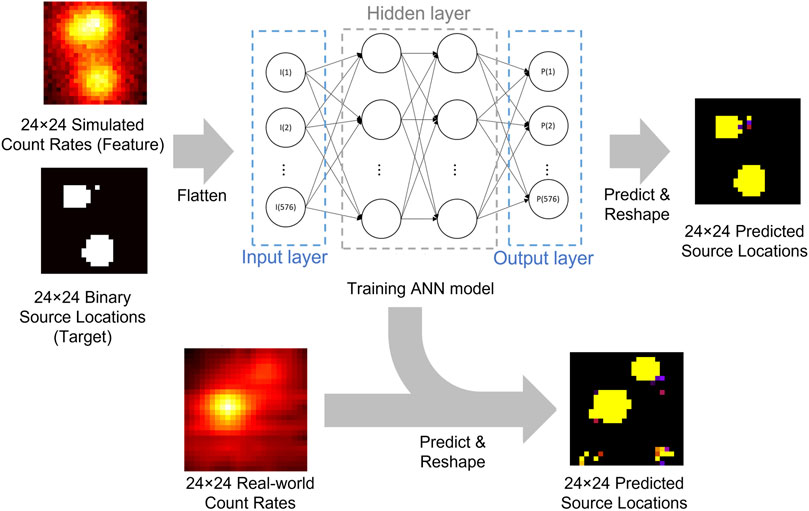
FIGURE 1. Conceptual diagram of the hotspot investigation algorithm.

The ANN is composed of a flattening layer to convert the two-dimensional data array into one-dimensional data before training, two hidden layers, and an output layer (Yegnanarayana, 2009). The first hidden layer uses the activation function of the rectified linear unit (ReLU), and the second layer uses a sigmoid function. A binary cross-entropy loss function is used to train the model to classify whether radioactive sources exist or not. Therefore, the model predicts the hotspots by using the count rates in the scanning intervals. The shape of the output from the model is same with the flattened input which corresponds to 576 × 1, and then, the output is reshaped to 24 × 24 to create image-like results. After the ANN is sufficiently trained by the dataset produced by simulation, the experimentally measured count rate data are used and predicted by the model. The performance of the model is evaluated by these real-world data. For summary, this model takes count rates in the pixels as the input, and it classifies whether each pixel has elevated radioactivity or not. Therefore, each count rate can be considered as a sample. Therefore, the model performance metrics such as accuracy, precision, and recall are estimated in an image that contains 576 samples.

2.2 Training data production

The number of samples should be sufficient to train a deep learning model. In general, a few thousand samples are required to train the learning model and validate it. However, data acquisition at this level of a source condition is too complex to carry out via an experiment. One scanning data include 24 × 24 count rates, and too much physical time is needed for the experiment. For the training of the ANN model, input (or feature) and answer (or target) datasets are required. It is important to have input data with a clear tendency with regard to the target data so as correctly to train the model data. For these reasons, we obtained the count rate data through a computational simulation and checked whether the model learns and predicts the locations of hotspots well. In this way, the model predicts hotspot locations when using an experimentally obtained count rate data.

Monte Carlo N-Particle 6 (MCNP6) was used for the particle transportation simulation (Goorley et al., 2012). The detector was composed of NaI(Tl) with a density of 3.67 g/cm³. Both the diameter and height of the detector were 7.62 cm. The target scanning area was a 100 cm² × 100 cm² concrete wall with a density of 2.3 g/cm³. The face of the detector was located at a distance of 10 cm from the wall. The detector was initially positioned at a starting point (4, 4), then moved in steps of 4 cm to emulate scanning, and finally reached the ending point (96, 96). In this way, 24 × 24 data points in total were acquired. The circular source was randomly positioned in the concrete wall area, and the source diameter was randomly sampled with a range of 0–15 cm. The source was uniformly distributed on the defined diameter with a depth of 1 cm. The radionuclide was ¹³⁷Cs, which emits mono-energy photons at 662 keV. Figure 2 shows examples of the randomly positioned circular sources and count rate data recorded by the scanning simulation. The black and white colors in each pixel represent the count rate data, and the orange circle, which represents the area of the source, is overlapped on the count rate data. The count rate data and the source position were well matched. Based on this, binary target datasets were produced in which all pixels touched by the source region were set to 1, while those without sources were set to 0.

FIGURE 2

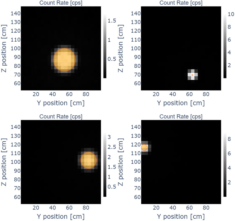
FIGURE 2. Examples of randomly positioned circular sources and their count rates obtained by the MCNP scanning simulation.

In total, 100 randomly generated single circle sources were simulated through MCNP6. The Y-position and Z-position of each source were randomly sampled from 0 to 100 cm and from 50 to 150 cm, respectively, when the X-direction was perpendicular to the wall. The scanning data with a single source were not a real-world case because there can be multiple source points in the scanning area. If a neural network model is trained with only single-source data, the accuracy for predicting multiple sources will be poor. Therefore, the input data with a single source were randomly sampled two, three, four, and five times in each case, yielding 1,000 combinations each to increase the number of samples and the responsiveness to multiple sources. By merging these combinations, 4,100 samples including single and multiple sources were prepared in this augmentation process. When preparing the datasets with n combinations, the fractions were randomly sampled to have a standard deviation of 1/5n to determine the deviation of the radioactivity with the data after combining and then normalized. Similar to the input datasets, 4,100 answer datasets were prepared but binarized, meaning that all non-zero cells were set to 1. The input and answer datasets were split into the training and test datasets with a ratio of 4:1. The model was trained by the training datasets, and the source position was predicted using the test datasets. The predicted results were compared with the test answer datasets with the same index.

2.3 Effects of the collimator and random background noise

The collimator shields the detector from extraneous photons but allows activity from a specified area of contamination to reach the detector. A short-pitch collimator can reduce scattered photons, and a long-pitch collimator can define the field-of-view of the detector. Given these characteristics, collimators are mainly used in radiographic imaging. During the process of producing the training data, two different conditions of the detector, with and without a collimator, were used in the test.

The random background count rate is inevitable during experimental measurements. The results from the Monte Carlo simulation only include count rates from defined radiation sources. In cases where an ANN model is trained with clear data without a background count rate, the predicted result will not be accurate if experimentally acquired input data, which include the background count rate, are used for prediction. Therefore, the data used for training should include random background noise to be similar to experimentally acquired data. If a detector has a collimator, a corresponding shield of the same thickness should cover it. The background count rates for the NaI(Tl) detector were experimentally estimated. The background count rates with and without a 2-cm lead collimator were estimated to be 5,082 and 24,969 cpm, respectively. Considering a scanning interval of 2 s, the average background counts for the corresponding scanning intervals were 169 ± 13 and 832 ± 29 counts. These background counts were randomly sampled and added to the count rate obtained from the tally.

To sum up, three datasets for training were produced: one without a background count rate with a collimator, one with a background count rate with a collimator, and one with a background count rate without a collimator. The first can represent the ideal case, while the latter two are closer to reality.

2.4 Experimental scanning test and application

A situation with sources placed on a wall with scanning along the wall was simulated. Figure 3 presents the arrangement of the detector and source on a wall for the experiment and the sources used in the experiment. In this case, a 100 cm² × 100 cm² grid paper was attached onto the wall, and two surface sources were attached onto the grid paper at arbitrary positions. The isotopes of the surface sources were ¹³⁷Cs and ⁶⁰Co with a surface area of 10 × 10 cm² in a square shape (Eckert & Ziegler). Their corresponding activities were 3,589 and 3,109 Bq, according to the decay rate from the reference date. From point (4, 4), moving by 4 cm, we reached point (96, 96) by measuring 10 s at each point. In this way, 24 × 24 count rate data were acquired in total. As with the data produced by the computational simulation, the data here were normalized and imaged. The imaged data were used as inputs for the model, and the source location was predicted.

FIGURE 3

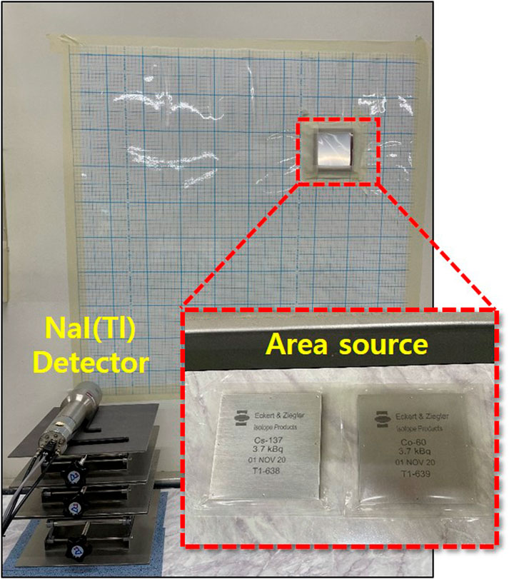
FIGURE 3. Arrangement of the detector and source on a wall for the experiment and the sources used in the experiment.

As a reference for the detection system, the scan minimum detectable concentration (scan MDC) was calculated by Eq. 1 (Abelquist and Brown, 1999).

$\text{scan}\text{MDC}=\frac{d^{\prime }\times \sqrt{b_i}\times \left(\frac{60}{i}\right)}{\sqrt{p}\times CPMR\times ERC}.(1)$

Here, d′ is the index of sensitivity, b_i is the background count in the measurement interval of i, p is the surveyor efficiency, CPMR denotes the ratio of counts per minute relative to the exposure rate, and ERC is the exposure-rate-to-concentration ratio. The index of the sensitivity value is determined according to the ratio of true positives and false positives. The index of the sensitivity value corresponding to 95% true positives and 25% false positives is 2.32. The scanning intervals were assumed to be 2 s in the computational simulation case and 10 s for the experimental case. The index of sensitivity and the scanning interval can be changed according to the requirements, considering the expected contamination level of the target area. The ¹³⁷Cs scan MDCs with a scanning interval of 2 s including and not including the collimator were estimated to be 8.20 and 17.62 Bq/g, respectively. For ⁶⁰Co, they were correspondingly 8.07 and 3.92 Bq/g. For the experiment case with a scanning interval of 10 s and not including the collimator, the scan MDCs were estimated to be 7.88 Bq/g and 3.61 Bq/g for ¹³⁷Cs and ⁶⁰Co, respectively. The corresponding ERCs were estimated to be .719 and 2.70 (nGy/h)/(Bq/g) in the given source condition.

3 Results and discussion

Figure 4 shows 10 predicted results using the ANN model trained with datasets without background noise. The column on the left represents the input count rate data, the middle column represents the source position predicted by the ANN model, and the column on the right represents the correct answer of the source position. The brightness of the input image differed according to the source, given the different relative intensities. In the predicted results, the colors represent the different probabilities of the prediction, with yellow, red, purple, and black spots correspondingly representing over 90%, around 60%, around 30%, and 0%, respectively. Hence, purple and black indicate no radioactive sources in the area, red represents a questionable or gray region, and yellow represents a clear presence of a radioactive source. Most sources were correctly predicted, except for cases where the difference in the fractions among sources was very large. Because the input data included no random background noise, the differences in the counting rates in the input data are relatively more highlighted by the difference in the strength of the source.

FIGURE 4

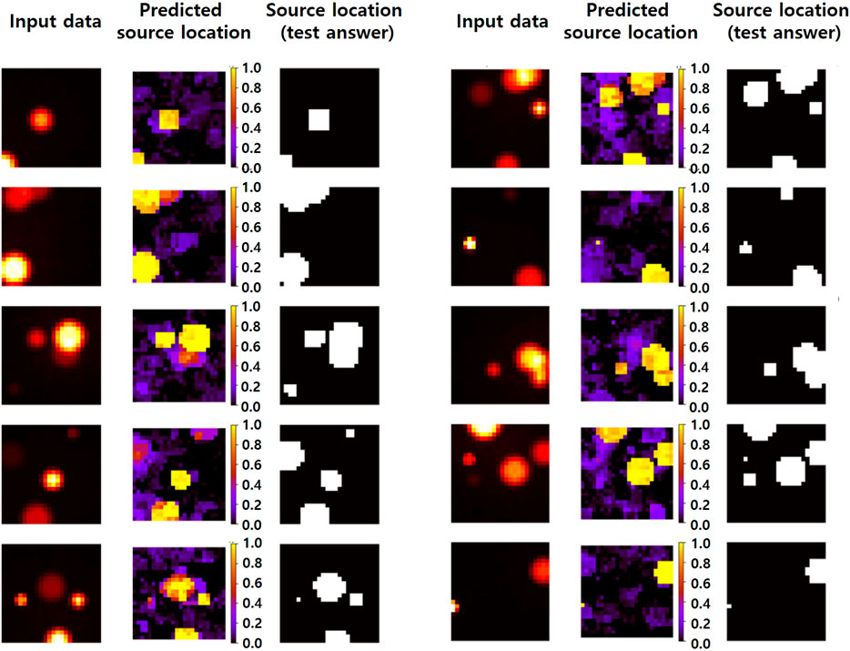
FIGURE 4. Predicted results using the ANN model trained with datasets without background noise. Image of the input count rate data (left) and predicted source position (middle), and the answer image of the source position (right) are shown.

Figure 5 shows the predicted results using the ANN model trained with datasets with random background noise and a collimator. The source rates were assumed to be 10, 1, .1, and .01 Bq/g for each circular source. As mentioned in the ‘Training data production’ section, the single-source datasets were mixed, and the radioactivity of each source had deviations. In the cases with a radioactivity concentration of 10 Bq/g, the source position is discriminable with the human eye. On the other hand, in other cases with lower concentrations, it is difficult to find the source position intuitively. However, the ANN model could correctly predict these source positions. It is assumed to be able to predict much better than when there was no random background noise. Considering that the scan MDC was on the order of few Bq/g, it is possible to find low-level hotspots not found by the existing scanning methods when the proposed algorithm is applied.

FIGURE 5

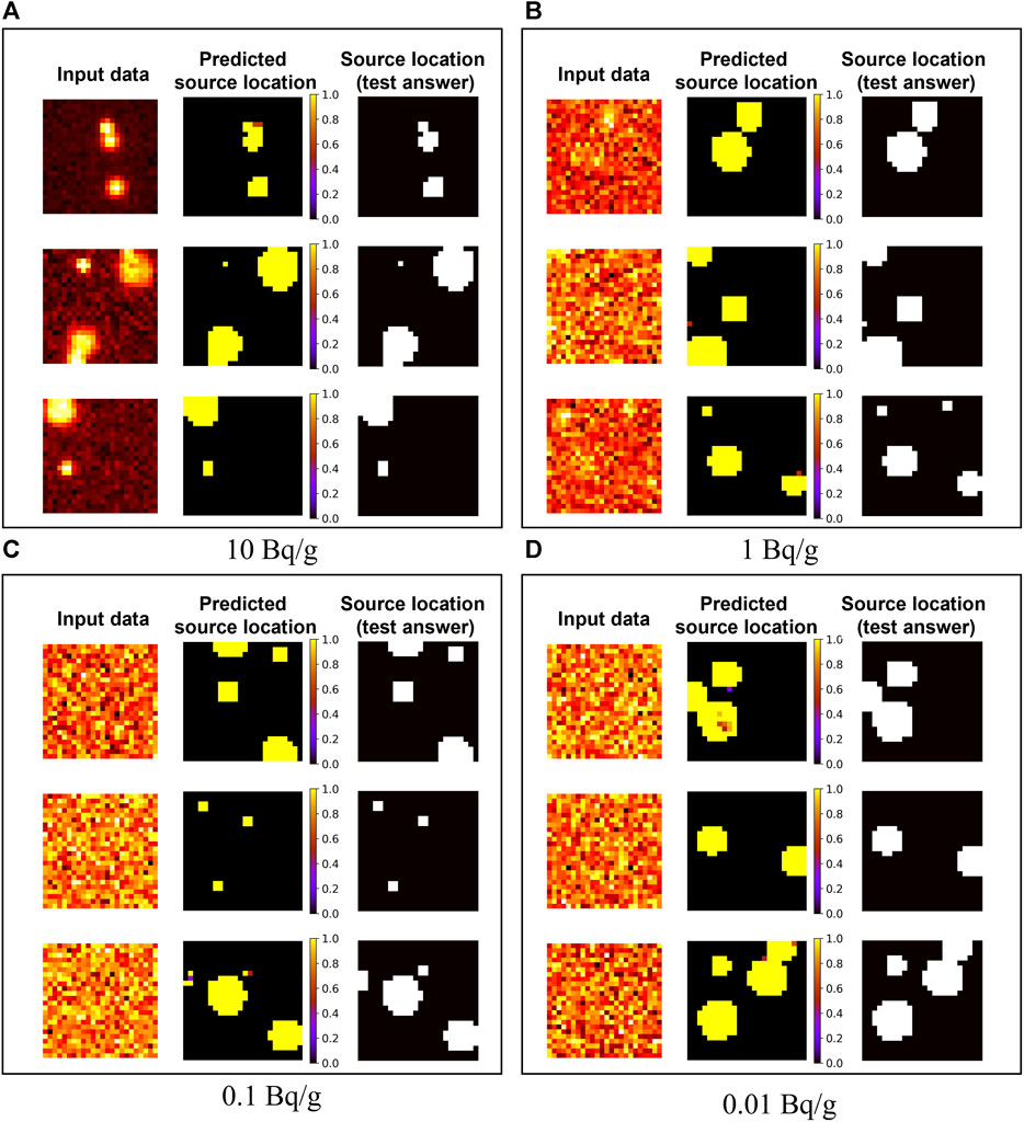
FIGURE 5. Predicted results using the ANN model trained by datasets with random background noise and equipped with a collimator. The radioactivity concentrations were as follows: (A) 10 Bq/g, (B) 1 Bq/g, (C) .1 Bq/g, and (D) .01 Bq/g.

Figure 6 shows the predicted results when using the ANN model trained by datasets with random background noise but without a collimator. Because no collimator was used, the bright points in the input data were more widely spread and were larger than the defined source area. Compared to Figure 5, for some source positions, the prediction probability was low. Specifically, relatively small source positions were predicted with lower probability. It was also confirmed that there are more prediction points with low probabilities displayed in purple.

FIGURE 6

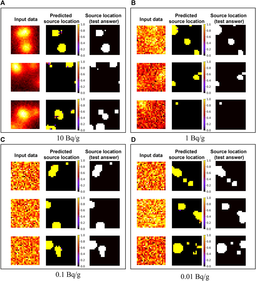
FIGURE 6. Predicted results using the ANN model trained with datasets with random background noise without a collimator. The radioactivity concentrations were (A) 10 Bq/g, (B) 1 Bq/g, (C) .1 Bq/g, and (D) .01 Bq/g.

Figure 7 shows the predicted result using the model with experimentally acquired count rate data. The model was trained with a dataset with background noise and no collimator, which was the condition most similar to that in the experiment. The first column shows experimentally acquired count rate input data, the second column represents the picture of the source arrangement, and the third and the fourth columns represent the predicted source locations. The third and fourth columns were predicted by differently trained models which used datasets with concentrations of 10 and 1 Bq/g, respectively. When using the model trained with the 10 Bq/g dataset, it has a smaller number of high-probability pixels, but it has some false positive pixels. Otherwise, when in case of the 1 Bq/g dataset, it has a larger area of high-probability pixels, which means that there are many false positive pixels near the true-source points. The accuracies with a threshold of .99 for three experimental data from top to bottom are .929, .943, and .918 for 10 Bq/g; .and 906, .870, and .888 for 1 Bq/g, respectively.

FIGURE 7

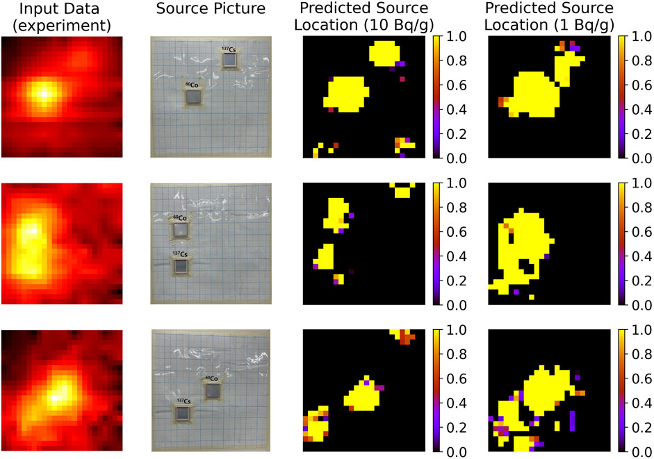
FIGURE 7. Predicted results with experimentally acquired input datasets. An image of the input dataset (Column 1), picture of the source arrangement (Column 2), and hotspot locations predicted using the model trained by scanning simulation data with concentrations of 10 Bq/g (Column 3) and 1 Bq/g (Column 4).

The source position of ⁶⁰Co was manually discriminable in the input data image; however, ¹³⁷Cs was difficult to discriminate because the data were normalized, and the relatively high intensity of ⁶⁰Co dominated the datasets. Therefore, the position of the bright points due to the ¹³⁷Cs source appears to have shifted. This can lead to a misrepresentation of the hotspot position. The probability prediction was relatively low compared to the simulation-only results. The experimental error was included in the dataset in this case, while the detector was moved manually. Each pixel needed to receive data at precise intervals to reflect the shape of the source accurately. If data can be acquired while moving at a constant speed, akin to a robot head used in optical devices, it will be possible to predict hotspots more accurately.

Figure 8 shows the receiver operation characteristic (ROC) curve and precision–recall curve with models that are trained by datasets with different concentrations. The model trained by the 10 Bq/g dataset shows the best performance with the highest area under curve (AUC) of .975. From a regulatory point of view, a frequency of type II errors (i.e., false negative rate) of .05 or less may be required. It implies that the model should show a certain level of precision where the recall is .95 or more, and the model trained on the 10 Bq/g dataset satisfies this criterion. In the case of 10 Bq/g, it has a surficial concentration of about 23 Bq/cm², and the surface source used in the experiment has a surficial concentration of about 35.9 Bq/cm². Therefore, models trained using a high-concentration dataset performed better. When applied in the field, if a model trained by the expected concentration of hotspots is used in consideration of the site condition, the prediction with high performance will be achieved. Based on the fact that the model trained with the simulated dataset at 1/30 of the concentration (1 Bq/g) used in the experiment also showed an accuracy of .87 or more, the proposed method shows tolerance to the concentration of the training dataset.

FIGURE 8

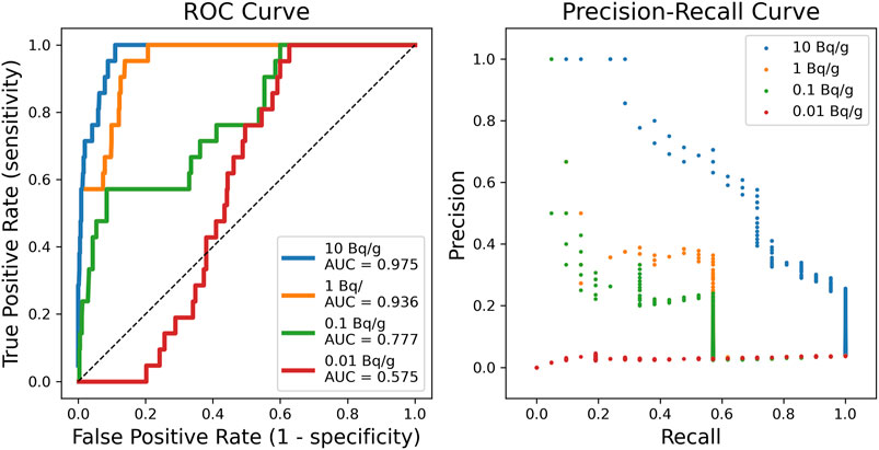
FIGURE 8. Receiver operation characteristic (ROC) curve (left) and precision–recall curve (right) with models that are trained by datasets with different concentrations.

In the scanning survey to measure the hotspots, a measurement point with a counting rate higher than that of MDCR is taken as a hotspot, but the proposed method has the advantage of imaging the data after scanning and finding hotspots with lower concentrations than the scan MDC through data correlations among the pixels in the image. In terms of the absorbed dose, it is possible to distinguish hotspots at the level of several nGy/h. In addition, it is possible to minimize unnecessary decontamination by adjusting the size of the hotspot in the data spread widely by scattered rays. One consideration for in-field use is that the measurement location and pixelization must be accurate. The cause of the relatively poor prediction performance in the experiment was the measurement location, which did not precisely match with the pixel. Therefore, when using in a small area, a specified area can be scanned using an automated robotic arm, or when using a large area, a data correction method must also be considered so that data can be entered into the correct grid through the Global Positioning System (GPS) (Adsley et al., 2004).

Table 1 summarizes the recent SCAN MDC analysis research results and describes the types of detectors, measured nuclides, and results.

TABLE 1

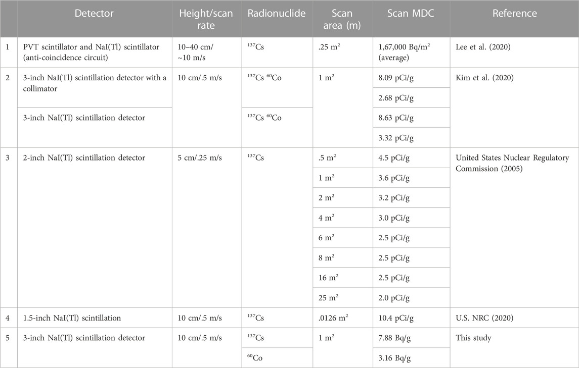
TABLE 1. Case study for the SCAN MDC analysis.

The method proposed here undertakes training and prediction based on the overall counts of the spectrum. This is performed because it is difficult to predict nuclides through the full-energy absorption peak because the time needed to determine the amount of data per pixel is very short due to the scanning rate. It is expected that hotspot locations can be identified more precisely if operated together with nuclide identification in combination with methods for detecting nuclides in low radioactivity or spectra with poor energy resolutions. Efforts to realize this are currently underway (Daniel et al., 2020; Jeon et al., 2020).

4 Conclusion

This study proposed an applicability of the in situ residual radioactive hotspot detection methodology using a constantly moving detection system with a deep learning model trained by simulated count rate data. The method was based on creating an image from scanning data and ANN-based deep learning. The scanned data were transformed into a 24 × 24 image and utilized for training and predictions. The ANN model was trained using data produced by a Monte Carlo simulation. The ANN model was trained and tested in several situations, including those with no background, with background noise, and a collimator, and with background noise and no collimator. When the data included random background noise, the hotspot position could be accurately predicted despite the fact that the activity of the source was lower than the scan MDC of the detecting condition. However, when multiple sources were spotted in the scanning region, if the amounts of deviation among the radioactivity levels of the sources were large, hotspots with lower activities were predicted at low probabilities or were not found. The method was validated by experimentally acquired data. The positions of the sources were well predicted. The advantages and limitations to the proposed method are as follows. Importantly, it is an ANN model trained with simulation data, and it can predict with high accuracy, even using experimental data. Furthermore, it is a great advantage that it can detect contaminated areas that are lower than the existing scan MDC. However, the limitation is that it cannot be predicted, or the accuracy is low in multi-sourced scans. As a challenge, we have a plan for the automation system of the low-activity radioactivity measurement and use it directly at the dismantling site to verify its performance. This methodology can easily be applied to an existing detection system simply by software applications including the algorithm and modifying the scanning process for imaging. This work is meaningful for the development of artificial neural networks and deep learning systems, which provide valuable insights and guidelines for future progress in a final status scan survey of nuclear decommissioning and contaminated sites.

Data availability statement

The original contributions presented in the study are included in the article/supplementary material; further inquiries can be directed to the corresponding author.

Author contributions

JB, SH, and BS contributed to the conception and design of the study. JB, CR, and SM carried out the experiments and simulations. Also, JB and SM contributed to manuscript revision under the supervision of BS, CR, and SH. All authors contributed to the discussion of experiments and simulation results.

Funding

This work was supported by the National Research Foundation of Korea (NRF) Grant funded by the Ministry of Science and ICT (NRF-2020M2C9A1068162 and RS-2022-00154985). Also, this work was supported by the Korea Institute of Energy Technology Evaluation and Planning (KETEP) and the Ministry of Trade, Industry & Energy (MOTIE) of the Republic of Korea (No. 20203210100190) and partially supported by the Nuclear Global Fellowship Program through the Korea Nuclear International Cooperation Foundation (KONICOF) funded by the Ministry of Science and ICT.

Conflict of interest

The authors declare that the research was conducted in the absence of any commercial or financial relationships that could be construed as a potential conflict of interest.

Publisher’s note

All claims expressed in this article are solely those of the authors and do not necessarily represent those of their affiliated organizations, or those of the publisher, the editors, and the reviewers. Any product that may be evaluated in this article, or claim that may be made by its manufacturer, is not guaranteed or endorsed by the publisher.

References

Abelquist, E. W., and Brown, W. S. (1999). Estimating minimum detectable concentrations achievable while scanning building surfaces and land areas. Health Phys. 76 (1), 3–10. doi:10.1097/00004032-199901000-00002

PubMed Abstract | CrossRef Full Text | Google Scholar

Abelquist, E. W., Clements, J. P., Huffert, A. M., King, D. A., Vitkus, T. J., and Watson, B. A. (2020). Minimum detectable concentrations with typical radiation survey instruments for various contaminants and field conditions. NUREG-1507 46, 3482.

Google Scholar

Abelquist, E. W. (2013). Decommissioning health physics:A handbook for MARSSIM users. London, United Kingdom: Routledge.

Google Scholar

Abu-Eid, R. B. (2012). Decommissioning survey and site characterisation issues and lessons learned. USNRC 57, 13223.

Google Scholar

Adsley, I., Davies, M., Murley, R., Pearman, I., and Scirea, M. (2004). 3D GPS mapping of land contaminated with gamma-ray emitting radionuclides. Appl. Radiat. isotopes 60 (2-4), 579–582. doi:10.1016/j.apradiso.2003.11.089

PubMed Abstract | CrossRef Full Text | Google Scholar

Ardiny, H., Witwicki, S., and Mondada, F. (2019). Autonomous exploration for radioactive hotspots localization taking account of sensor limitations. Sensors 19 (2), 292. doi:10.3390/s19020292

PubMed Abstract | CrossRef Full Text | Google Scholar

Colak, A. B., Shafiq, A., and Sindhu, T. N. (2022). Modeling of Darcy-Forchheimer bioconvective Powell Eyring nanofluid with artificial neural network. Chin. J. Phys. 77, 2435–2453. doi:10.1016/j.cjph.2022.04.004

CrossRef Full Text | Google Scholar

Cui, X., Wang, Q., Zhao, Y., Qiao, X., and Teng, G. (2019). Laser-induced breakdown spectroscopy (LIBS) for classification of wood species integrated with artificial neural network(ANN). Appl. Phys. B 125 (56), 56–12. doi:10.1007/s00340-019-7166-3

CrossRef Full Text | Google Scholar

Daniel, G., Ceraudo, F., Limousin, O., Maier, D., and Meuris, A. (2020). Automatic and real-time identification of radionuclides in gamma-ray spectra: A new method based on convolutional neural network trained with synthetic data set. IEEE Trans. Nucl. Sci. 67 (4), 644–653. doi:10.1109/tns.2020.2969703

CrossRef Full Text | Google Scholar

Gal, O., Gmar, M., Ivanov, O. P., Lainé, F., Lamadie, F., Le Goaller, C., et al. (2006). Development of a portable gamma camera with coded aperture. Nucl. Instrum. Methods Phys. Res. Sect. A Accel. Spectrom. Detect. Assoc. Equip. 563 (1), 233–237. doi:10.1016/j.nima.2006.01.119

CrossRef Full Text | Google Scholar

Galib, S., Bhowmik, P., Avachat, A., and Lee, H. (2021). A comparative study of machine learning methods for automated identification of radioisotopes using NaI gamma-ray spectra. Nucl. Eng. Technol. 53 (12), 4072–4079.,

CrossRef Full Text | Google Scholar

Goorley, T., James, M., Booth, T., Brown, F., Bull, J., Cox, L., et al. (2012). Initial MCNP6 release overview. Nucl. Technol. 180 (3), 298–315. doi:10.13182/nt11-135

CrossRef Full Text | Google Scholar

Hong, S. B., Hwang, D. S., Seo, B. K., and Moon, J. K. (2014). Practical application of the MARSSIM process to the site release of a Uranium Conversion Plant following decommissioning. Ann. Nucl. Energy 65, 241–246. doi:10.1016/j.anucene.2013.11.018

CrossRef Full Text | Google Scholar

Hong, S. B., Lee, K. W., Park, J. H., and Chung, U. S. (2011). Application of MARSSIM for final status survey of the decommissioning project. J. korean Radioact. waste Soc. 9, 107–111. doi:10.7733/jkrws.2011.9.2.107

CrossRef Full Text | Google Scholar

Huang, L., Zhou, Y., Han, Y., Hammitt, J. K., Bi, J., and Liu, Y. (2013). Effect of the Fukushima nuclear accident on the risk perception of residents near a nuclear power plant in China. Proc. Natl. Acad. Sci. U. S. A. 110 (49), 19742–19747. doi:10.1073/pnas.1313825110

PubMed Abstract | CrossRef Full Text | Google Scholar

Jeon, B., Lee, Y., Moon, M., Kim, J., and Cho, G. (2020). Reconstruction of Compton edges in plastic gamma spectra using deep autoencoder. Sensors 20 (10), 2895. doi:10.3390/s20102895

PubMed Abstract | CrossRef Full Text | Google Scholar

Kim, J. H., Cho, G. S., Lee, J. J., Hong, S. B., Lee, E. J., Seo, B. K., et al. (2020). Study on improvement of scan survey system performance using collimator. Trans. Korean Nucl. Soc. 787, 4733.

Google Scholar

Kim, J., Lim, K. T., Kim, J., Kim, C.-j., Jeon, B., Park, K., et al. (2019). Quantitative analysis of NaI(Tl) gamma-ray spectrometry using an artificial neural network. Nucl. Instrum. Methods Phys. Res. Sect. A Accel. Spectrom. Detect. Assoc. Equip. 944, 162549. doi:10.1016/j.nima.2019.162549

CrossRef Full Text | Google Scholar

Kurtz, J. E. (2017). Technical basis document:detection capability for radiological field instruments, Washingtonriver protection solutions. RPP-53865 3, 65.

Google Scholar

Lee, C., Park, S.-W., and Kim, H. R. (2020). Development of mobile scanning system for effective in-situ spatial prediction of radioactive contamination at decommissioning sites. Nucl. Instrum. Methods Phys. Res. Sect. A Accel. Spectrom. Detect. Assoc. Equip. 966, 163833. doi:10.1016/j.nima.2020.163833

CrossRef Full Text | Google Scholar

Lee, K. W., Hong, S. B., Park, J. H., and Chung, U. S. (2010). Final status of the decommissioning of research reactors in Korea. J. Nucl. Sci. Technol. 47 (12), 1227–1232. doi:10.1080/18811248.2010.9720990

CrossRef Full Text | Google Scholar

Li, L. N., Liu, X. F., Yang, F., Xu, W. M., Wang, J. Y., and Shu, R. (2021). A review of artificial neural network based chemometrics applied in laser-induced breakdown spectroscopy analysis. Artificial 180, 106183.

CrossRef Full Text | Google Scholar

Okada, K., Tadokoro, T., Ueno, Y., Nukaga, J., Ishitsu, T., Takahashi, I., et al. (2014). Development of a gamma camera to image radiation fields. Prog. Nucl. Sci. Technol. 4, 14–17. doi:10.15669/pnst.4.14

CrossRef Full Text | Google Scholar

Owens, A. S., Engel, K. M., Benton, P. H., Smith, W. F., and Bailey, E. N. (2018). Characterization report for ORISE south campus building SC-13 oak ridge. Tenn. 18-HEE-0996 55, 1772.

Google Scholar

Sato, Y., Ozawa, S., Terasaka, Y., Minemoto, K., Tamura, S., Shingu, K., et al. (2020). Remote detection of radioactive hotspot using a Compton camera mounted on a moving multi-copter drone above a contaminated area in Fukushima. J. Nucl. Sci. Technol. 57 (6), 734–744. doi:10.1080/00223131.2020.1720845

CrossRef Full Text | Google Scholar

Sato, Y., Tanifuji, Y., Terasaka, Y., Usami, H., Kaburagi, M., Kawabata, K., et al. (2018). Radiation imaging using a compact Compton camera inside the fukushima daiichi nuclear power station building. J. Nucl. Sci. Technol. 55 (9), 965–970. doi:10.1080/00223131.2018.1473171

CrossRef Full Text | Google Scholar

Shafiq, A., Colak, A. B., Sindhu, T. N., Al-Mdallal, Q. M., and Abdeljawad, T. (2021a). Estimation of unsteady hydromagnetic Williamson fluid flow in a radiative surface through numerical and artificial neural network modeling. Sci. Rep. 11, 14509. doi:10.1038/s41598-021-93790-9

PubMed Abstract | CrossRef Full Text | Google Scholar

Shafiq, A., Colak, A. B., and Sindhu, T. N. (2021b). Designing artificial neural network of nanoparticle diameter and solid–fluid interfacial layer on single-walled carbon nanotubes/ethylene glycol nanofluid flow on thin slendering needles. Int. J. Numer. Methods Fluids 93, 3384–3404. doi:10.1002/fld.5038

CrossRef Full Text | Google Scholar

Shafiq, A., Colak, A. B., Sindhu, T. N., and Muhammad, T. (2022). Optimization of Darcy-forchheimer squeezing fluow in nolinear stratified fluid under convective conditions with artificial neural network. Heat. Transf. Res. 53 (3), 67–89. doi:10.1615/heattransres.2021041018

CrossRef Full Text | Google Scholar

Sibille, L., Seifert, R., Avramovic, N., Vehren, T., Spottiswoode, B., Zuehlsdorff, S., et al. (2019). ¹⁸F-FDG PET/CT Uptake classification in Lymphoma and Lung Cancer by using deep convolutional neural networks. Radiology 294 (2), 445–452. doi:10.1148/radiol.2019191114

PubMed Abstract | CrossRef Full Text | Google Scholar

Suzuki, Y., Yamaguchi, M., Odaka, H., Shimada, H., Yoshida, Y., Torikai, K., et al. (2013). Three-dimensional and multienergy gamma-ray simultaneous imaging by using a Si/CdTe Compton camera. Radiology 267 (3), 941–947. doi:10.1148/radiol.13121194

PubMed Abstract | CrossRef Full Text | Google Scholar

Takahashi, J., Tamura, K., Suda, T., Matsumura, R., and Onda, Y. (2015). Vertical distribution and temporal changes of 137Cs in soil profiles under various land uses after the Fukushima Dai-ichi Nuclear Power Plant accident. J. Environ. Radioact. 139, 351–361. doi:10.1016/j.jenvrad.2014.07.004

PubMed Abstract | CrossRef Full Text | Google Scholar

United States Nuclear Regulatory Commission (2005). Maine yankee's license termination plan(LTP), sectopm 5, final status survey plan.

Google Scholar

Vico, A. M., Noguerales, M. C., Rodriguez, L., and Alvarez, A. (2021). Clearance of building of a former uranium concentrates plant. Ann. Nucl. Energy 159, 108313. doi:10.1016/j.anucene.2021.108313

CrossRef Full Text | Google Scholar

Yegnanarayana, B. (2009). Artificial neural networks. PHI Learn. Pvt. Ltd. 53, 33213.

Google Scholar