 Chuansijia Tao
94% of researchers rate our articles as excellent or good
Learn more about the work of our research integrity team to safeguard the quality of each article we publish.
Find out more
ORIGINAL RESEARCH article
Front. Energy Res. , 22 November 2021
Sec. Advanced Clean Fuel Technologies
Volume 9 - 2021 | https://doi.org/10.3389/fenrg.2021.791542
This article is part of the Research Topic Advanced Technologies in Flow Dynamics and Combustion in Propulsion and Power View all 25 articles
Solidity and camber angle are key parameters with a primary effect on airfoil diffusion. Maximum thickness location has a considerable impact on blade loading distribution. This paper investigates correlations of maximum thickness location, solidity, and camber angle with airfoil performance to choose maximum thickness location quickly for compressor airfoils with different diffusion. The effects of maximum thickness location, solidity, and camber angle on incidence characteristics are discussed based on abundant two-dimensional cascade cases computed through numerical methods. Models of minimum loss incidence, total pressure loss coefficient, diffusion factor, and static pressure rise coefficient are established to describe correlations quantitatively. Based on models, dependence maps of total pressure loss coefficient, diffusion factor, and static pressure rise coefficient are drawn and total loss variation brought by maximum thickness location is analyzed. The study shows that the preferred selection of maximum thickness location can be the most forward one with no serious shock loss. Then, the choice maps of optimal maximum thickness location on different design conditions are presented. The optimal maximum thickness locates at 20–35% chord length. Finally, a database of optimal cases which can meet different loading requirements is provided as a tool for designers to choose geometrical parameters.
•Performance prediction models containing maximum thickness location is established, which can be used in compressor preliminary design.
•Choice maps of maximum thickness location and solidity are found on three different conditions, where camber angle, diffusion factor, or static pressure rise is constant respectively.
•A database of optimal maximum thickness location is provided for designers to meet different design requests.
With the increase of stage loading, the area coverage of boundary layer separation enlarges and disordered vortex structures become more complicated within the flow passage (Sun et al., 2018; Hu et al., 2021; Ju et al., 2020). To achieve good aerodynamic performance, employing effective flow control approaches is necessary both in rotors and stators for the highly loaded aero-engine compressor (Wang et al., 2021). The low-reaction design method is proposed to simplify the sophisticated flow control strategy (Qiang et al., 2008; Sun et al., 2019; Sun et al., 2020; Sun et al., 2021). For a highly loaded low-reaction stage, both the inlet Mach number and the static pressure rise of the stator significantly increase. In this case, the high subsonic stator airfoil design with high flow turning which can achieve low loss-level, increase efficiency and static pressure rise capability becomes a huge challenge (Zhang et al., 2019).
When inlet Mach number increases to a certain degree, supersonic flow appears at local region of suction surface and brings sharp rise of loss (Shi and Ji, 2021). It is called supercritical flow condition when incoming flow is high subsonic and transonic flow exists in the passage. With shock-free and controlled diffusion features, controlled-diffusion airfoil (CDA) introduced in the early 1980s was originally designed for supercritical cascades (Dunker et al., 1984; Niederdrenk et al., 1987; Elazar and Shreeve, 1990; Steinert et al., 1991; Jiang et al., 2015). As CDA blades were primarily developed for aero-engines but not the optimum solution for heavy-duty gas turbines, Köller et al. (2000) and Kusters et al. (2000) designed a high subsonic compressor airfoil family (Ma ≤ 0.8, θ≤ 30°, e/b = 25%). The optimization results demonstrated that the well-controlled front loading airfoil obtained good performance through promoting early transition without strong laminar separation. Besides, it is conducive to reducing the adverse pressure gradient and the loading at the rear region of suction side. Sieverding et al. (2004) transferred and adapted the preceding design system to industrial compressors and the optimized airfoils (Ma = 0.5, e/b = 25%) were generated. The results indicated that as the maximum thickness location moved forward, the peak velocity position on the suction side migrated forwards, and stabilized boundary layer is the reason why front-loading airfoils present good performance. Wang et al. (2020) investigated the evolution of vortex structures and separated flow transition process in front-loaded airfoil through large eddy simulations. As the laminar separation was suppressed on the suction surface of the front-loaded airfoil, the associated vortex dynamics was weakened. Hence, the high level of Reynolds shear stresses recedes.
Although previous conclusions for front-loading airfoils are effective, most optimization research objects are dispersive and lack of revealing the universal rules of parameter selection. When facing different design requirements, it is difficult to achieve a quick front-loading blade profile design. Moreover, these questions must be raised: What kind of flow problems will occur when the maximum thickness position moves forward? Is there a limit to the forward movement of the maximum thickness position? What is the effect of cascade key parameters on the influence brought by forward movement of maximum thickness position? The systematic study of cascade geometrical parameters is helpful to reflect the influence rules of key geometrical parameters on airfoil aerodynamic performance and reveal the flow evolution mechanism. In this situation, it is necessary to build up performance prediction models for supercritical airfoils, which include maximum thickness location and key geometrical parameters. The results of models contribute to revealing the generality of maximum thickness location selection and providing a tool of blade profile selection for mean-line and through-flow design.
For high-load aero-engine compressor design, solidity and camber angle are key geometrical parameters in preliminary design, which have a remarkable influence on flow turning capacity, blade loading, and working range (Howell, 1945; Zweifel, 1945; Carter, 1950; Lieblein et al., 1953; Johnsen and Bullock, 1965; Britsch, 1979). An increase of solidity could achieve high flow turning, but increases the number of blades and profile loss (Sans et al., 2014). To meet the needs of empirical solidity inputs in mean-line and through-flow design, performance prediction models including solidity which can be used in multistage axial flow compressor are needed (Larosiliere et al., 2002; Horlock and Denton, 2005; Burberi et al., 2020). Sans et al. (2014) updated the correlations for controlled diffusion blades and extended their application to the high Mach number flow regimes. Bruna and Cravero chose inlet flow angle, inlet Mach number, AVDR, Reynolds number, and solidity as model parameters to study profile loss (Ma1 = 0.5–0.84, σ = 0.625–2, θ = 37.4°–43.4°) (Bruna et al., 2006). Xu and Du established performance characteristics prediction models for the curved blade containing solidity and camber angle in NACA65 compressor cascade (Ma1 = 0.2–0.6, σ = 1.2–1.8, θ = 30°–60°) (Xu et al., 2018), and integrated aspect ratio into the models in the follow-up research (Xu et al., 2019).
As an attempt to provide a reference for compressor preliminary design, this paper investigates rules of maximum thickness location selection matching cascade key parameters. Several camber angles are selected to investigate different typical flow problems for the generality of the conclusion. The in-house program introduced in reference (Li, 2007) is used for the generation of profiles. The numerical calculation carried out in abundant two-dimensional linear cascades has been successfully applied for performance evaluations and flow phenomena detections. The evolution of performance parameters (ωo, Do, and Cp2o) at minimum loss incidence versus geometrical parameters (σ, e/b, and θ) is studied. The flow mechanism leading to the performance differences is analyzed based on the calculated performances and flow details. Then performance parameters are described in function of geometrical parameters. Based on polynomial models, dependence maps ofωo, Do, and Cp2o and the effect of e/b on them are discussed. In addition, choice maps of optimal e/b at selected θ, Do, or Cp2o are presented respectively. Finally, a database of all the optimal e/b is provided for designers with different demands as a tool to choose parameters.
The investigated blade profile is used in the stator of the second stage of a three-stage compressor. The curve of the camber line is described by a quartic polynomial and normalized by axial chord length, as shown in Figure 1A. It is well controlled to arrange the blade loading chordwise distribution and to alter the deviation angle. Two cubic polynomial curves connected at maximum thickness location are used to describe the thickness distribution, as shown in Figure 1B. The d1, d2 are the leading edge and trailing edge radius. The variables K1, K2 are the rate of thickness changing along the chord at leading edge and trailing edge. The e is the location of maximum thickness, while e/b is normalized by chord.
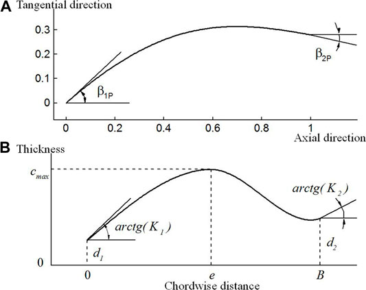
FIGURE 1. Curves of camber and thickness distribution (A) Camber line; (B) Thickness distribution.
Geometrical parameters and flow conditions of the cascade are shown in Table 1. Maximum thickness and its position are normalized by chord length. Chord length, maximum thickness and inlet curvature of camber line has been optimized in the previous design of blade profile. Cascade geometrical parameters (σ, e/b, and θ) are changed in the ranges which cover the usually used values in industry applications. Effects of e/b and θ on profiles are shown in Figure 2. Figure 3 shows the axial distribution of the thickness and suction side curvature of the blade at θ = 40°. As shown in the figure, the curvature of the suction side has a step, whose position is obviously related to e/b. The suction side curvature increases before the step but reduces after it with the forward migration of e/b.
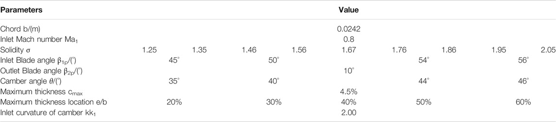
TABLE 1. Parameters and flow conditions of research.
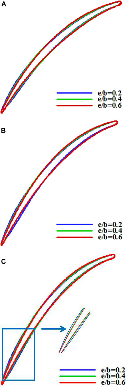
FIGURE 2. Profiles with different cambers and maximum thickness locations (A) θ = 40°; (B) θ = 44°; (C) θ = 46°.
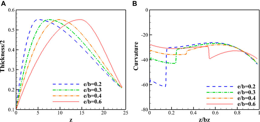
FIGURE 3. Axial distribution of profile thickness (A) and the curvature of suction side (B).
The structured grid is generated by the IGG/AutoGrid5 module of the NUMECA software package. As shown in Figure 4, a mixed O-and H-block is used for the computation domain. The inlet of the computational domain is located 100% chord length ahead of the leading-edge. The outlet of the computational domain is set 100% chord length behind the trailing-edge with a buffer zone. The measurement plane location is 40% chord length behind the trailing-edge for complete wake development. The thickness of the first grid layer is 10−6 m, and 5 × 10⁻⁶ m near the hub and shroud, which can insure y+<3 at solid wall in all cases and satisfy the solving demands of the selected turbulence model in this paper.
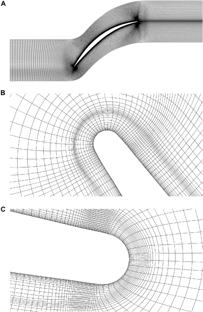
FIGURE 4. Configuration of calculation mesh grids (A) Grids diagram; (B) Mesh grids at the leading edge; (C) Mesh grids at the trailing edge.
With such a topology structure, a grid independence study is carried out with different grid nodes number, including seven meshes with respectively from about 45 to 140 thousands cells. As shown in Figure 5, when further refining the mesh grid with grid number beyond 100 thousands, the results almost have no modification. Therefore, the spanwise node number adopted is 5 in this study, and the total grid node number is about 109 thousands.
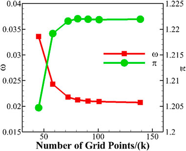
FIGURE 5. Effect of grid points number on the loss and static preesure ratio.
The code solver FINE™ EURANUS is used to solve the Reynolds-Averaged Navier-Stokes equations with finite volume form. The governing equation for the relative velocities in the rotating frame can be expressed as:
where
where the superscripts “-” and “∼” are the time average value and density weighted average value, respectively; wi is the xi component of the relative velocity; E is the total energy; p* is the total pressure; δij is the Kronecker number; τij is the Reynolds stress; and qi is the heat flux component. The contributions of the Coriolis and centrifugal forces are contained in the source item vector Q, which is given by:
where ω is the angular velocity of the relative frame of reference; r is the radius; and
The MOGA profile in literature (Song and Ng, 2006) is selected to validate the calculation methods of the two-dimensional cascade. Several turbulence models were adopted to show the effect of turbulence models on the simulation accuracy at Ma = 0.77 in Figure 6A. It can be seen that the trend of numerical simulation is basically consistent with experiments. The Spalart-Allmaras turbulence model is employed, as it provides high robustness and good compromise in accuracy for the prediction of complex flows (Spalart and Allmaras, 1994). The simulations are fully turbulent without boundary layer transition effects.
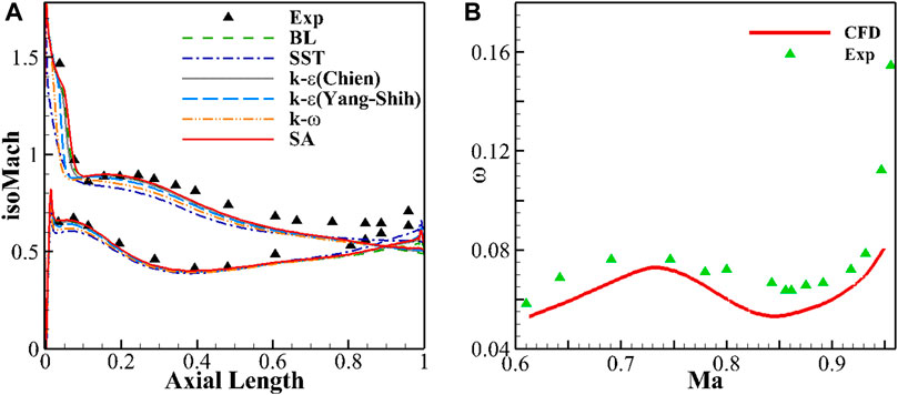
FIGURE 6. Comparison of numerical and experimental results (A) Isentropic Mach distribution of blade surface; (B) Total pressure loss versus inlet Mach number.
Besides, the space discrete form is TVD of the second-order upwind scheme, and Min-Mod flux limiter is adopted to enhance the scheme stability. The temporal discretization scheme is four-stage Runge-Kutta scheme, with multigrid solver and implicit residual smoothing method to accelerate the residual convergence.
Inlet boundary conditions are prescribed with total pressure (430 kPa), total temperature (440 K) and inflow angle. Free-slip and adiabatic conditions are imposed at the solid walls. Translational periodic boundary condition is used in the pitchwise direction. In the computations, the mass-flow specified at the outlet is modified to achieve the desired inlet Mach number. Non-reflecting boundary condition is used at inlet/outlet planes.
Based on Lieblein’s definition (Lieblein, 1955), the diffusion factor given in Eq. 4 is used to assess the loading of blades. In Eq. 4,
The effect of maximum thickness location (e/b), solidity (σ) and camber angle (θ) on airfoil performance are discussed, including minimum loss incidence (io), diffusion factor (Do), total pressure loss coefficient (ωo), and static pressure rise coefficient (Cp2o). Minimum loss incidence (io) refers to the incidence with minimum loss within the incidence range, while the other three performance parameters are obtained in this case.
Figure 7 shows incidence characteristics of total pressure loss coefficient and diffusion factor from negative to positive stall at different solidities (Ma1 = 0.8). It can be seen that as solidity increases, total pressure loss coefficient curves move up and rightwards, and diffusion factor curves migrate rightwards. Obviously, io, ωo and Do increase with solidity.
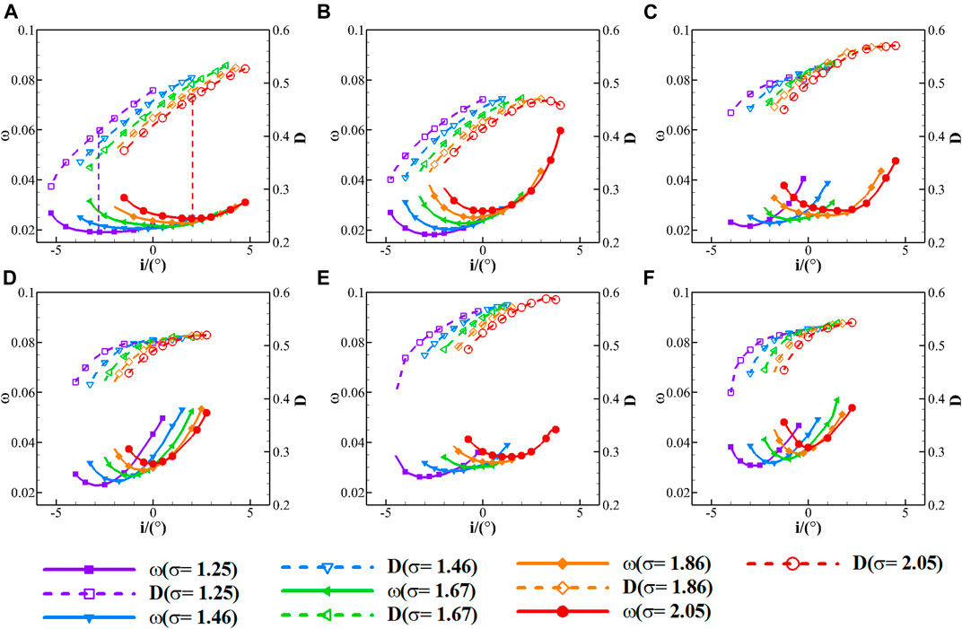
FIGURE 7. Influence of solidities on incidence characteristics of total pressure loss coefficient and diffusion factor (A) e/b = 0.2, θ = 40°; (B) e/b = 0.6, θ = 40°; (C) e/b = 0.2, θ = 44°; (D) e/b = 0.6, θ = 44°; (E) e/b = 0.2, θ = 46°; (F) e/b = 0.6, θ = 46°.
Figure 8 shows incidence characteristics of total pressure loss coefficient and diffusion factor with different camber angles (Ma1 = 0.8). It can be seen that as camber angle increases, incidence range shrinks, while both total pressure loss coefficient and diffusion factor curves move up, which means ωo and Do increase but io changes slightly.
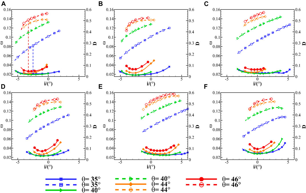
FIGURE 8. Influence of camber angles on incidence characteristics of total pressure loss coefficient and diffusion factor (A) e/b = 0.2, σ = 1.25; (B) e/b = 0.6, σ = 1.25; (C) e/b = 0.2, σ = 1.67; (D) e/b = 0.6, σ = 1.67; (E) e/b = 0.2, σ = 2.05; (F) e/b = 0.6, σ = 2.05.
Figure 9 shows incidence characteristics of total pressure loss coefficient and diffusion factor with different maximum thickness locations (Ma1 = 0.8). It can be seen that when maximum thickness location moves upstream, positive incidence range increases and loss reduces, except for Figures 9A,C. As e/b increases, io and Do reduce but ωo increases.
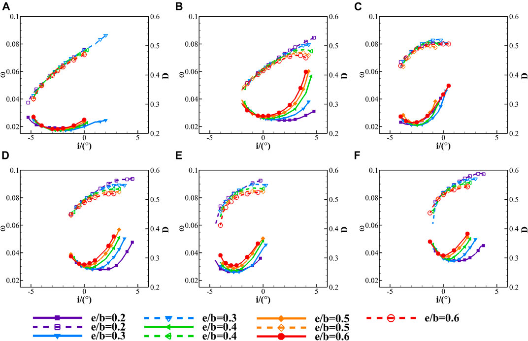
FIGURE 9. Influence of maximum thickness locations on incidence characteristics of total pressure loss coefficient and diffusion factor (A) θ = 40°, σ = 1.25; (B) θ = 40°, σ = 2.05; (C) θ = 44°, σ = 1.25; (D) θ = 44°, σ = 2.05; (E) θ = 46°, σ = 1.25; (F) θ = 46°, σ = 2.05.
It can be found that solidity (σ), camber angle (θ), and maximum thickness location (e/b) have impacts on two-dimensional cascade incidence characteristics. The trend of optimum incidence performance varying with cascade geometrical parameters will be discussed in detail afterward.
Supplementary Figure S10 shows io versus σ with different e/b and θ. It can be seen that as σ increases, io rises nearly linearly, except for the cases at e/b = 0.2, θ ≤ 40°. The trend is in accord with the results in reference (Sans et al., 2014). Supplementary Figure S11 shows io versus θ with different σ and e/b. It shows that the evolvement of io versus θ is quadratic almost for all e/b and σ. In most cases, io decreases slightly with an increasing θ, except for cases at e/b = 0.2, σ ≥ 1.46. In these cases, io decreases more significantly, which agrees with Supplementary Figure S10A. Supplementary Figure S12 shows io versus e/b with different σ and θ. It illustrates that the evolution of io with e/b is quadratic, reflecting in two different patterns. In the cases with big θ and small σ, io increases firstly and then decreases while e/b is enhanced. In the cases with small θ and big σ, io decreases as e/b increases.
Supplementary Figure S13 shows ωo versus σ with different e/b and θ. It illustrates that ωo almost increases linearly with σ. It is because that a rise in a number of blades attracts linear increases of profile loss. Supplementary Figure S14 shows ωo versus θ with different e/b and σ. As θ rises, ωo decreases firstly and then increases, which can also be observed in Supplementary Figure S13. Supplementary Figure S15 shows ωo versus e/b with different σ and θ. It indicates that ωo decreases firstly and then increases with the rise of e/b, which presents quadratic curves except for some low-load cases. The minimum of ωo occurs at e/b = 0.2–0.3 and alters with σ and θ.
Supplementary Figure S16 shows Do versus solidity with different e/b and θ. As solidity is increasing, Do increases and then keeps constant with a quadratic trend. The influence of σ is very limited. It is because that the rise of io with σ causes an increase of blade load correspondingly and compensates for the decrease of blade load caused by σ. Another observation is that Do increases faster for lower cambers at e/b = 0.2, which is different from the reference (Sans et al., 2014). It is because that the e/b is different from that of the literature (Sans et al., 2014), while the observation in literature (Sans et al., 2014) agrees with the cases at e/b ≥ 0.3.
Supplementary Figure S17 shows Do versus θ with different e/b and σ. Do increases linearly as θ increases, which is a result of flow turning increase. Supplementary Figure S18 shows Do versus e/b with different σ and θ. It can be seen that Do varies quadratically with e/b, resembling curves of io versus e/b in Supplementary Figure S12.
Supplementary Figures S19–21 show Cp2o versus σ, θ, and e/b respectively. The trends of Cp2o evolution resemble these of Do in Supplementary Figures S16–18. Besides, it can be noticed that Cp2o is influenced more significantly than Do by σ.
This section aims at revealing how e/b affects the loss-level of the blade and transonic flow of airfoils with normal camber angle (θ ≤ 40°) without flow separation. Analysis indicates that the related flow mechanism is the same at θ = 35° and θ = 40°. For brevity, the cases with θ = 40° are selected to discuss here. As shown in Supplementary Figure S22, the e/b can cause a significant influence on velocity distribution at blade surface and load of the blade. With the upstream propagation of e/b, the position of suction peak velocity moves forward, and peak velocity increases, which result in the front-loaded velocity distribution. When e/b moves forward to a certain extent, the flow after the suction peak decelerates sharply. Besides, suction peak velocity increases with the reduction of solidity, which means a rise in blade loading.
As shown in Supplementary Figure S23, the flow separation does not occur in moderate-load blade passage. It can be observed through the flow field that the acceleration in the front portion of the passage amplifies with the upstream propagation of e/b. Shock wave generates when e/b moves forward to some extent. It indicates that the forward migration of e/b induces shock. In conjunction with Figure 3B, it can be attributed to that in the flow acceleration region before the shock (before 20% chord), the forward migration of e/b causes the increase of the curvature of the suction side, which is conducive to the flow acceleration. By comparing the flow field at different solidities, it can be found that the shock is easy to occur at low σ, which is caused by the increased suction peak velocity. In general, the forward migration of e/b and reduction of σ induces the generation of shock.
Supplementary Figure S24 illustrates the velocity gradient on the blade surface, which reflects viscous shear in the boundary layer. It can be seen that in the case without serious shock, the velocity gradient reduces with the forward migration of e/b in the most portion (30–80% chord), which indicates the weaker viscous shear. It is the reason why the small e/b reduces total pressure loss in the case without shock. By comparing with Figure 3B, it can be found that in the deceleration area after the suction peak velocity, the reduction of suction side curvature caused by the upstream propagation of e/b contributes to the lower gradient of velocity. In conjunction with analysis of flow field, how the e/b alteration influences loss of the blade is demonstrated: in the flow acceleration region before 20% chord, the forward migration of e/b induces the generation of shock; while in the deceleration region after the suction peak velocity, the upstream propagation of e/b contributes to the weaker viscous shear.
This section illustrates how e/b affects the loss of the blade and transonic flow of high-load airfoils with higher camber angle (θ ≥ 44°) with flow separation. For brevity, the cases with θ = 46° are selected to discuss for the clearer difference. As shown by Supplementary Figure S25, the trend of velocity distribution on the blade surface and load of the blade caused by e/b and σ are the same as normal airfoils (θ ≤ 44°, as shown in Supplementary Figure S22). The case e/b = 0.31 is the optimal e/b at θ = 46°, σ = 1.25. It should be mentioned that the rise of the camber angle generates a slight drop in suction peak velocity.
Supplementary Figure S26 illustrates the flow field at θ = 46°. It can be observed that compared with normal airfoils, flow separation exists at the rear portion of the blade (behind 80% chord). The scale of separation shrinks with the upstream migration of e/b. Besides, the effects of e/b and σ on acceleration flow are the same as that in normal airfoils. It should be noted that the strength of supersonic flow at θ = 46° is weaker than that of θ = 40°, which can be attributed to the lower peak velocity in Supplementary Figure S25.
The influence of e/b on boundary layer behavior is used to explain the reason for loss-level. It can be observed in Supplementary Figure S27 that the influence of e/b on velocity gradient and viscous shear agrees with the trend reflected in Supplementary Figure S24. Especially, reverse flow occurs in the area where the velocity gradient is close to zero. At small solidity (σ = 1.25), the forward migration of e/b delays the onset of boundary layer separation.
Supplementary Figure S28 reflects the boundary layer growth before separation. It can be noticed that low e/b contributes to the stabilized boundary layer, which reflects in the delay of the onset of rapid growth of boundary layer. The total pressure distribution of blade wake shown in Supplementary Figure S29 also confirms that the high total pressure loss region of blade wake significantly shrinks with the forward migration of e/b. In general, small e/b conduces to the drop of the loss (caused by viscous friction) and the separation scale of high-load airfoils, although contributes to the generation of shock.
Based on the discussion above, it can be inferred that io, ωo, Do and Cp2o change with σ, θ, and e/b, and their correlations can be described by such quadratic multiple regression model as Eq. 7. The variable
Supplementary Figure S30 shows the comparison of results obtained by models and CFD calculations, in which the horizontal axis and vertical axis represent CFD results and model predicting results. The red lines imply that the results predicted by models are equal to CFD calculations, while blue dots are close to them.
Supplementary Figure S31 shows errors of the model predicting results compared with CFD calculations. The error of minimum loss incidence (Δio) is defined as
The established models help to obtain numerous continuous data in the investigation sample space and to explore the correlations maps of parameters. The distribution of minimum loss (ωo) is given in Supplementary Figure S32 when θ is constant. Three axes represent e/b, θ, and σ, while the blue color represents low ωo. It can be seen in Supplementary Figure S32 that ωo rises sharply when θ increases over 44°. For constant θ, the low loss area exists at low σ and upstream e/b. Because the camber angle is determined in premier compressor design, it is necessary to explore the correlations of e/b and σ at selected θ.
Quantitative analysis of total loss variation brought by e/b is necessary in order to evaluate the impact of e/b. It can be found in Supplementary Figure S32 that for constant θ and σ, the maximum loss is mostly at e/b = 0.6. The total loss variation (δωo) is defined as
Supplementary Figure S33 displays the distribution of total loss variation (δωo) caused by the alteration of e/b (θ = 40°), as well as contours of Do and Cp2o. Three axes of Supplementary Figure S33 represent σ, e/b, and ωo, while the red color represents high total loss variation. For each σ, there is a maximum δωo (namely, the minimum ωo) case, whose e/b is called as optimal e/b (e/bopt). Such cases compose the black line named as (δωo) max, θ = 40°.
In Supplementary Figure S33, contours of Do and Cp2o at constant θ are displayed under the contour of δωo. The solid black lines and dashed ones represent contours of Do and Cp2o respectively. It can be seen that the upstream move of e/b leads to an increase of Do and Cp2o, which means that the optimum e/b reduces loss and increases diffusion.
All the cases with the maximum of δωo composing the surface of e/bopt for selected θ and σ are given in Supplementary Figure S34. The points on the surface produce lower loss than those with the same θ and σ but off the surface. It can be observed that e/bopt locates at 25–35% chord. This observation includes but is not limited to the reference (Koller et al., 1999; Kusters et al., 2000; Sieverding et al., 2004).
The distribution of optimal e/b is illustrated in Supplementary Figure S35, while δωo of e/bopt is shown in Supplementary Figure S36. It can be observed that e/bopt moves downstream when θ or σ decreases and the shock generates more easily. It can achieve more than a 10% reduction of total pressure loss at θ ≥ 44°. Thus, compared with normal-load airfoils, smaller e/b is preferred to produce excellent aerodynamic performance in high-load cascades, while total loss variation caused by e/bopt is more significant.
The cases with e/bopt (θ = 40° or 46°, σ = 1.25 or 2.05) in Supplementary Figure S35 are selected to verify the accuracy of e/bopt predicted by the model. Their velocity distribution and boundary layer behaviors are depicted in details in Supplementary Figures S22–29. In conjunction with the previous analysis, it can be found that the e/bopt is the most forward e/b without serious shock loss. Therefore, the preferred selection of e/b for the high subsonic airfoil can be suggested as the most forward e/b with no serious shock loss.
Because diffusion factor indicates blade load, it is necessary to explore correlations of parameters at different Do. As a result of the predominant effect of θ on Do, the isosurfaces of Do in Supplementary Figure S37 are nearly horizontal and similar to those of θ in Supplementary Figure S32.
It can be noticed in Supplementary Figure S37 that for constants Do and σ, the maximum loss occurs at e/b = 0.6. The δωo is still defined as
Supplementary Figure S38 displays δωo and ωo versus σ and e/b when Do is the constant, as well as contours of Cp2o and θ. At each σ, there is a maximum δωo case, whose e/b is the optimal e/b. The black line, named as (δωo) max, Do = 0.5, consists of such cases. It can be noticed that e/bopt moves upstream when σ increases.
In Supplementary Figure S38, contours of θ and Cp2o are drawn as solid black lines and dashed ones under the contour of δωo. It can be seen that the upstream move of e/b leads to θ and Cp2o reduction. It means that e/bopt achieves lower ωo and Cp2o and maintains Do with lower θ than e/b = 0.6 at the same σ.
All the cases with e/bopt at selected σ and Do among the sample space are given in Supplementary Figure S39. The points on the surface produce lower loss than those with the same Do and σ but off the surface. It can be observed that the e/bopt locates at a 20–35% chord.
The situation where Cp2o is constant is discussed in this part. Because Cp2o rises with the increase of Do, the isosurfaces of Cp2o in Supplementary Figure S40 are similar to those of Do in Supplementary Figure S37. Solidity has a significant effect on Cp2o, which causes the difference between isosurfaces of Do and Cp2o.
Since highest loss occurs at e/b = 0.6 for selected Cp2o and σ, δωo is defined as
Supplementary Figure S41 displays δωo and ωo versus σ and e/b when Cp2o is constant, as well as contours of Do and θ. The black line which is named as (δωo) max, Cp2o = 0.4 consists of the cases with maximum δωo at each σ. At selected Cp2o, the optimal e/b moves forward as σ increases.
In Supplementary Figure S41, the solid black lines and dashed ones under the isosurface of Cp2o are contours of θ and Do. Because θ reduces and Do increases as e/b decreases, e/bopt achieves lower loss and higher Do with lower θ than e/b = 0.6 at the same Cp2o and σ.
The cases with e/bopt are given in Supplementary Figure S42 and produce lower loss than those with the same Cp2o and σ but off the surface. The e/bopt locates at a 20–35% chord.
All the optimal e/b that can meet the three different kinds of design requirements (selected θ, Do, or Cp2o) are contained by a database, whose flow chart is shown in Supplementary Figure S43. The design requirement is regarded as a restriction, and correlation of optimal e/b, ωo, Do, Cp2o, and θ with σ on the line of (δωo)max are depicted in maps. According to needed performance parameters (such as ωo or Cp2o), σ can be chosen appropriately and input. Then corresponding e/bopt and performance parameters (ωo, Do, Cp2o) predicted by models are provided as the output.
The program interface of the database is shown in Supplementary Figure S44. When the θ input is 44°, maps of e/bopt, ωo, Do and Cp2o versus σ are shown below the θ input box in Supplementary Figure S44A. It can be seen that as σ increases, e/bopt moves forward, and ωo, Do, Cp2o rise. When the desired σ (such as 1.3) is input, corresponding e/bopt, ωo, Do and Cp2o are indicated by red stars on the curves, and their values are displayed on the right side. Small σ (for example, σ = 1.25) can be chosen to reduce ωo, when e/bopt is at 32% chord length. Large σ (for example, σ = 2.05) is available to improve Do and Cp2o, when e/bopt is at 23% chord length.
The database is also useful when the design goal is to achieve a certain Do (for example, Do = 0.45) or Cp2o (for example, Cp2o = 0.4). When Do is selected, the effects of σ on e/bopt, ωo, θ and Cp2o are given below the Do input box in Supplementary Figure S44B. It can be seen that as σ increases, e/bopt moves forward, the corresponding θ decreases, while ωo and Cp2o rise. When Cp2o is selected, the effects of σ on e/bopt, ωo, θ and Do are presented below the Cp2o input box in Supplementary Figure S44C. As σ increases, e/bopt moves forward, corresponding θ and Do decrease, and ωo rises. Therefore, the predetermined Cp2o can be achieved at σ = 1.25 with the lowest ωo, when e/bopt is at 33% chord length.
This paper aims to investigate the influence of geometrical parameters (e/b, θ, σ) on the aerodynamic performance (Do, ωo, Cp2o) of high subsonic stator airfoil. Numerical investigation indicates that optimization of e/b can lead to a considerable reduction of loss level at minimum loss incidence condition. The key conclusions are as follows:
1) Substantial two-dimensional cascade cases are simulated through validated numerical methods. It is indicated that Do, ωo, and Cp2o versus σ are linear, but quadratic versus e/b. Do and Cp2o versus θ are linear, while ωo versus θ is quadratic.
2) In the flow acceleration region before the 20% chord, the forward migration of e/b causes the increase of the curvature of the suction side. It is conducive to the flow acceleration and induces the generation of shock. While in the deceleration region after the suction peak velocity, the reduction of suction side curvature caused by the upstream propagation of e/b contributes to the drop of loss and separation scale. Therefore, the preferred selection of e/b can be suggested as the most forward e/b with no serious shock loss.
3) Quadratic multiple regression models of performance parameters are established. The models help to obtain the optimal e/b surfaces at selected θ, Do or Cp2o. The results show that when e/bopt locates at 20–35% chord, δωo is maximum. As θ, Do, or Cp2o increase, δωo becomes more significant. So, the selection of e/b has an important effect on high-load blade profile.
4) A database is established to meet design requests, which provides optimal e/b according to the selected θ, Do, Cp2o and σ. When θ is selected, maps of performance parameters (ωo, Do, Cp2o) versus σ are depicted, according to which σ can be appropriately chosen. When selected σ is input, corresponding optimal e/b and performance parameters predicted by models are presented as the output. The database also helps when the design request is selected Do or Cp2o.
The original contributions presented in the study are included in the article/Supplementary Material, further inquiries can be directed to the corresponding author.
CT provides innovation, numerical simulation experiment, model establishment and writing for this article. XD provides financial support and guidance about the content of the article. JD and ZW contributes similar to XD. YL has engaged in some technical work.
This research is supported by the National Natural Science Foundation of China (Grant No. 51906049), China Postdoctoral Science Foundation (No. 2020M671672) and the National Science and Technology Major Project (No. 2017-II-0007-0021).
JD was employed by Hangzhou Turbine Power Group Co., Ltd.
The remaining authors declare that the research was conducted in the absence of any commercial or financial relationships that could be construed as a potential conflict of interest.
All claims expressed in this article are solely those of the authors and do not necessarily represent those of their affiliated organizations, or those of the publisher, the editors and the reviewers. Any product that may be evaluated in this article, or claim that may be made by its manufacturer, is not guaranteed or endorsed by the publisher.
The Supplementary Material for this article can be found online at: https://www.frontiersin.org/articles/10.3389/fenrg.2021.791542/full#supplementary-material
Britsch, W. R. (1979). Effects of Diffusion Factor, Aspect Ratio and Solidity on Overall Performance of 14 Compressor Middle Stages. Washington: National Aeronautics and Space Administration.
Bruna, D., Cravero, C., and Turner, M. G. (20062006). The Development of an Aerodynamic Performance Prediction Tool for Modern Axial Flow Compressor Profiles. Proc. ASME Turbo. Expo 6, 113–122. doi:10.1115/gt2006-90187
Burberi, C., Michelassi, V., Del Greco, A. S., Lorusso, S., Tapinassi, L., Marconcini, M., et al. (2020). Validation of Steady and Unsteady CFD Strategies in the Design of Axial Compressors for Gas Turbine Engines. Aerosp. Sci. Technol. 107. doi:10.1016/j.ast.2020.106307
Carter, A. D. S. (1950). The Low Speed Performance of Related Aerofoils in Cascades. A.R.C. Tech. Report, Report No.R.55. Washington: NGTE.
Dunker, R., Rechter, H., Starken, H., and Weyer, H. (1984). Redesign and Performance Analysis of a Transonic Axial Compressor Stator and Equivalent Plane Cascades with Subsonic Controlled Diffusion Blades. J. Eng. Gas Turbines Power 106, 279–287. doi:10.1115/1.3239560
Elazar, Y., and Shreeve, R. P. (1990). Viscous Flow in a Controlled Diffusion Compressor Cascade with Increasing Incidence. J. Turbomach. 112, 256–265. doi:10.1115/1.2927642
Horlock, J. H., and Denton, J. D. (2005). A Review of Some Early Design Practice Using Computational Fluid Dynamics and a Current Perspective. J. Turbomach. 127, 5–13. doi:10.1115/1.1650379
Howell, A. R. (1945). Fluid Dynamics of Axial Compressors. Proc. Inst. Mech. Eng. 153, 441–452. doi:10.1243/pime_proc_1945_153_049_02
Hu, H. D., Yu, J. Y., Song, Y. P., and Chen, F. (2021). The Application of Support Vector Regression and Mesh Deformation Technique in the Optimization of Transonic Compressor Design. Aerosp. Sci. Technol. 112, 106589. doi:10.1016/j.ast.2021.106589
I. A. Johnsen, and R. O. Bullock (Editors) (1965). Aerodynamic Design of Axial-Flow Compressors (Washington: Scientific and Technical Information Division, National Aeronautics and Space Administration), 36.
Jiang, B., Zheng, Q., Zhang, H., Zhang, X. L., Chen, Z. L., Qiu, Y., et al. (2015). Advanced Axial Compressor Airfoils Design and Optimization. Asme. Turbo. Expo. Turbine Tech. Conf. Exposition 2a, 11. doi:10.1115/gt2015-43846
Ju, Z. Z., Teng, J. F., Zhu, M. M., Ma, Y. C., Qiang, X. Q., Fan, L., et al. (2020). Flow Characteristics on a 4-stage Low-Speed Research Compressor with a Cantilevered Stator. Aerosp. Sci. Technol. 105, 106033. doi:10.1016/j.ast.2020.106033
Köller, U., Mönig, R., Küsters, B., and Schreiber, H.-A. (2000). Development of Advanced Compressor Airfoils for Heavy-Duty Gas Turbines - Part I: Design and Optimization. J. Turbomach. 122, 397–405. doi:10.1115/1.1302296
Kusters, B., Schreiber, H. A., Koller, U., and Monig, R. (2000). Development of Advanced Compressor Airfoils for Heavy-Duty Gas Turbines - Part II: Experimental and Theoretical Analysis. J. Turbomach. 122, 406–414. doi:10.1115/99-GT-096
Larosiliere, L. M., Wood, J. R., Hathaway, M. D., Medd, A. J., and Dang, T. Q. (2002). Aerodynamic Design Study of Advanced Multistage Axial Compressor. Washington: National aeronautics and space administration cleveland oh glenn research center.
Li, S. B. (2007). “Design of Highly Loaded Dihedral Stator and Investigation on the Aerodynamic Stage Performance in an Axial Transonic Compressor,” Doctor Thesis (China: Harbin Institute of Technology).
Lieblein, S. (1955). Aerodynamic Design of Axial-Flow Compressors: VI-experimental Flow in Two-Dimensional Cascades. Cleveland, OH: NACA Research Memorandum, Lewis Flight Propulsion Laboratory.
Lieblein, S., Schwenk, F. C., and Broderick, R. L. (1953). Diffusion Factor for Estimating Losses and Limiting Blade Loadings in Axial-Flow-Compressor Blade Elements. Cleveland, OH: NACA Research Memorandum, Lewis Flight Propulsion Laboratory.
Niederdrenk, P., Sobieczky, H., and Dulikravich, G. S. (1987). Supercritical Cascade Flow Analysis with Shock-Boundary Layer Interaction and Shock-free Redesign. J. Turbomach. 109, 413–419. doi:10.1115/1.3262121
Qiang, X. Q., Wang, S. T., Feng, G. T., and Wang, Z. Q. (2008). Aerodynamic Design and Analysis of a Low-Reaction Axial Compressor Stage. Chin. J. Aeronaut. 21, 1–7. doi:10.1016/S1000-9361(08)60001-1
Sans, J., Resmini, M., Brouckaert, J. F., and Hiernaux, S. (20142014). Numerical Investigation of the Solidity Effect on Linear Compressor Cascades. Proc. Asme. Turbo. Expo. Turbine Tech. Conf. Exposition 2a, 15. doi:10.1115/gt2014-25532
Shi, H., and Ji, L. (2021). Leading Edge Redesign of Dual-Peak Type Variable Inlet Guide Vane and its Effect on Aerodynamic Performance. Proc. Inst. Mech. Eng. G: J. Aerospace Eng. 235, 1077–1090. doi:10.1177/0954410020966168
Sieverding, F., Ribi, B., Casey, M., and Meyer, M. (2004). Design of Industrial Axial Compressor Blade Sections for Optimal Range and Performance. J. Turbomach. 126, 323–331. doi:10.1115/1.1737782
Song, B., and Ng, W. F. (2006). Performance and Flow Characteristics of an Optimized Supercritical Compressor Stator cascade. J. Turbomach. 128, 435–443. doi:10.1115/1.2183316
Spalart, P. R., and Allmaras, S. R. (1994). A One-Equation Turbulence Model for Aerodynamic Flows. Seattle: Rech. Aerospatiale, 5–21.
Steinert, W., Eisenberg, B., and Starken, H. (1991). Design and Testing of a Controlled Diffusion Airfoil Cascade for Industrial Axial Flow Compressor Application. J. Turbomach. 113, 583–590. doi:10.1115/1.2929119
Sun, S., Chen, S., Liu, W., Gong, Y., and Wang, S. (2018). Effect of Axisymmetric Endwall Contouring on the High-Load Low-Reaction Transonic Compressor Rotor with a Substantial meridian Contraction. Aerospace Sci. Tech. 81, 78–87. doi:10.1016/j.ast.2018.08.001
Sun, S. J., Wang, S. T., and Chen, S. W. (2020). Design, Modification and Optimization of an Ultra-high-load Transonic Low-Reaction Aspirated Compressor. Aerosp. Sci. Technol. 105, 105975. doi:10.1016/j.ast.2020.105975
Sun, S. J., Wang, S. T., and Chen, S. W. (2019). The Influence of Diversified Forward Sweep Heights on Operating Range and Performance of an Ultra-high-load Low-Reaction Transonic Compressor Rotor. Energy 194, 116857. doi:10.1016/j.energy.2019.116857
Sun, S. J., Wang, S. T., Zhang, L. X., and Ji, L. C. (2021). Design and Performance Analysis of a Two-Stage Transonic Low-Reaction Counter-rotating Aspirated Fan/compressor with Inlet Counter-swirl. Aerosp. Sci. Technol. 111, 106519. doi:10.1016/j.ast.2021.106519
Wang, M. Y., Li, Z. L., Yang, C. W., Han, G., Zhao, S. F., and Lu, X. G. (2020). Numerical Investigations of the Separated Transitional Flow over Compressor Blades with Different Loading Distributions. Aerosp. Sci. Technol. 106, 106113. doi:10.1016/j.ast.2020.106113
Wang, Z. A., Chang, J. T., Li, Y. F., and Kong, C. (2021). Investigation of Shock Wave Control by Suction in a Supersonic cascade. Aerosp. Sci. Technol. 108, 106382. doi:10.1016/j.ast.2020.106382
Xu, W., Du, X., Tao, C., Wang, S., and Wang, Z. (2019). Correlation of Solidity, Aspect Ratio and Compound Lean Blade in Compressor cascade Design. Appl. Therm. Eng. 150, 175–192. doi:10.1016/j.applthermaleng.2018.12.167
Xu, W., Du, X., Wang, S., and Wang, Z. (2018). Correlation of Solidity and Curved Blade in Compressor cascade Design. Appl. Therm. Eng. 131, 244–259. doi:10.1016/j.applthermaleng.2017.12.003
Zhang, L., Wang, S., and Zhu, W. (2019). Application of Endwall Contouring in a High-Subsonic Tandem cascade with Endwall Boundary Layer Suction. Aerospace Sci. Tech. 84, 245–256. doi:10.1016/j.ast.2018.08.041
Zweifel, O. (1945). The Spacing of Turbo-Machine Blading, Especially with Large Angular Deflection. Brown Boveri Rev. 32, 436–444.
h/b aspect ratio
h blade height
b chord
R2 coefficient of determination
kk curvature of camber
D diffusion factor
P* total pressure
T* total temperature
v velocity
c thickness
i incidence angle
Ma Mach number
e/b maximum thickness location
Re Reynolds number
P static pressure
Cp2 static pressure rise coefficient
βp blade angle
θ camber angle
ω the total pressure loss coefficient
ΔD errors of diffusion factor
δω Total loss variation
δD improvement of diffusion factor
δCp2 improvement of static pressure rise coefficient
δθ improvement of camber angle
Δv velocity-difference
σ solidity
Δi errors of incidence
ΔCp2 errors of static pressure rise coefficient
Δω errors of total pressure loss coefficient
o minimum incidence
Mod model
u tangential
1 inlet
2 outlet
max maximum
min minimum
Keywords: high subsonic compressor, blade profile, maximum thickness location, solidity, prediction model, database
Citation: Tao C, Du X, Ding J, Luo Y and Wang Z (2021) Maximum Thickness Location Selection of High Subsonic Axial Compressor Airfoils and Its Effect on Aerodynamic Performance. Front. Energy Res. 9:791542. doi: 10.3389/fenrg.2021.791542
Received: 08 October 2021; Accepted: 05 November 2021;
Published: 22 November 2021.
Edited by:
Bengt Sunden, Lund University, SwedenReviewed by:
Xiaoqing Qiang, Shanghai Jiao Tong University, ChinaCopyright © 2021 Tao, Du, Ding, Luo and Wang. This is an open-access article distributed under the terms of the Creative Commons Attribution License (CC BY). The use, distribution or reproduction in other forums is permitted, provided the original author(s) and the copyright owner(s) are credited and that the original publication in this journal is cited, in accordance with accepted academic practice. No use, distribution or reproduction is permitted which does not comply with these terms.
*Correspondence: Xin Du, xindu@hit.edu.cn
Disclaimer: All claims expressed in this article are solely those of the authors and do not necessarily represent those of their affiliated organizations, or those of the publisher, the editors and the reviewers. Any product that may be evaluated in this article or claim that may be made by its manufacturer is not guaranteed or endorsed by the publisher.
Research integrity at Frontiers
Learn more about the work of our research integrity team to safeguard the quality of each article we publish.