PM2.5 concentration simulation by hybrid machine learning based on image features

Air pollution significantly impacts human health, making the development of effective pollutant concentration assessment methods crucial. This study introduces a hybrid machine learning approach to simulate PM_2.5 mass concentration using outdoor images, offering an alternative to traditional observation techniques. The proposed method utilizes a convolutional neural network (CNN) to extract image features through transfer learning. The importance of these features is then evaluated using a random forest (RF) model. In addition, the extracted image features are combined with meteorological data (e.g., temperature (TEM), relative humidity (RHU), and sea level pressure (PRS_Sea)) and pollutant concentration data (hourly PM_2.5 concentrations from four monitoring stations) for complete ensemble empirical mode decomposition with adaptive noise (CEEMDAN) signal decomposition. This results in multiscale signals that are subsequently used in the hybrid machine learning model to simulate PM_2.5 concentrations. The results demonstrate that the ResNet50 training method, which extracts 64 image features, yields the best performance. An RF model is applied to the low-frequency signal, superimposed with the trend signal, while a Lasso regression model is used for the high-frequency signal. The combined approach produces superior simulation results than the RF model alone. Notably, image feature 23, PM_2.5 concentration from the Institute of Biological Products (IBP), and TEM are most influential for the high-frequency signal, with characteristic coefficients of 1.409, 0.380, and 0.318, respectively. For the low-frequency signals, image features 5 and 23, along with the PM_2.5 concentration from the Lanlian Hotel (LH), are the most significant, with importance values of 0.170, 0.137, and 0.125, respectively. The Lasso regression model (random forest model) has the function of high (low) value correction for high (low) frequency signal simulation, leading to more accurate simulation results. This study proposes a cost-effective method for accurately estimating PM_2.5 concentrations.

1 Introduction

The rapid development of urbanization and economy has rendered PM_2.5 pollution a significant environmental and social concern (Geng et al., 2015; Wang et al., 2021; Wang et al., 2018; Wilson et al., 2024). Prolonged exposure to elevated concentrations of PM_2.5 is associated with increased morbidity and mortality related to respiratory diseases (Pascal et al., 2014), cardiovascular diseases (Brook et al., 2010; Hayes et al., 2020), and cerebrovascular diseases (Leiva et al., 2013). Researchers have devised various methods and techniques to assess PM_2.5 concentrations in the atmosphere, with surface monitoring being the most prevalent and accurate approach for measuring PM_2.5 levels (Fang et al., 2016). However, the distribution of surface monitoring sites is often sparse and uneven, and the associated costs can be prohibitive, thereby constraining the real-time monitoring of PM_2.5 concentrations (Brauer et al., 2016; Carvalho, 2016; Hu et al., 2014). Aerosol optical thickness (AOT) is proportional to the number of particles in the air. AOT assessment of PM_2.5 concentration has become a widely used method for satellite derivatives (Beloconi et al., 2016). However, satellite-based data are not easily accessible and may have missing values in special conditions such as cloudy, snowy, and high-pollution days (Luo et al., 2020), and there are defects in the inversion of PM_2.5 concentration in the lower layers. Numerical simulations of PM_2.5 mass concentration, such as community multiscale air quality (CMAQ) and the Weather Research and Forecasting model coupled to Chemistry (WRF-Chem), rely on emission inventories and may lead to large deviations from the actual situation due to uncertainties in their estimation and analysis (Zhong et al., 2007), which often need objective observation to test.

Increased PM_2.5 levels contribute to a reduction in atmospheric visibility, with concentration exhibiting an inverse correlation with visibility (Wang et al., 2006). Visibility plays a significant role in determining the clarity of images. By examining the relationship between outdoor imagery and PM_2.5 mass concentration, a cost-effective assessment of PM_2.5 levels in the atmosphere can be achieved. Liaw et al. (2020) employed a series of image processing techniques alongside a simple linear regression model to estimate PM_2.5 concentration. In recent years, nonlinear predictive models, including deep learning and machine learning, have been increasingly developed and applied in the simulation and prediction of PM_2.5 concentrations. Luo et al. (2020) established an end-to-end hybrid evaluation model for PM_2.5 concentration based on convolutional neural networks (CNNs) and gradient boosting machines (GBM), utilizing imagery from the Shanghai Oriental Pearl in 2016. Zheng et al. (2020) utilized a deep CNN to process images, extracting features that characterize daily dynamic changes in the built environment, and employed a random forest (RF) regressor to estimate PM_2.5 concentration based on these extracted features in conjunction with meteorological data. Wang et al. (2024) introduced a hybrid deep learning model that integrates CNN and long short-term memory (LSTM) networks, leveraging the temporal continuity of air quality variations to estimate outdoor PM_2.5 concentration from surveillance images. The aforementioned studies indicate that deep learning technologies and machine learning models demonstrate strong performance in the domain of image processing for estimation purposes.

Research has indicated that hybrid models can amalgamate the strengths of two or more models, yielding superior performance compared to that of individual models (Li et al., 2017; Sun and Li, 2020; Wang et al., 2017). Hybrid models can be broadly categorized into simple hybrid models and decomposition-ensemble models (Jiang et al., 2021). In these models, nonlinear and non-stationary data are decomposed into components of varying time scales; each decomposed subseries is then trained and predicted individually, with the final predictions aggregated to produce an overall estimate (Du et al., 2020; Liu et al., 2020; Liu et al., 2019; Yang H. F. et al., 2020). Bai et al. (2019) proposed a decomposition-ensemble model that combines ensemble empirical mode decomposition (EEMD) with LSTM and demonstrated that this hybrid model outperforms both single feedforward neural networks and LSTM models in terms of the predictive accuracy. Similarly, Huang G. Y. et al. (2021) developed a decomposition-ensemble model based on empirical mode decomposition (EMD) and gated recurrent units (GRU), with results indicating that the hybrid model’s predictive performance surpasses that of individual models. For subsequences generated after signal decomposition and reconstruction, different models exhibit varying levels of accuracy in simulating results for subsequences with different frequencies. Therefore, it remains challenging to evaluate air quality using various machine learning models to simulate subsequences of differing frequencies and to integrate the final simulations effectively.

Lanzhou is characterized as a typical valley-type mountainous city (Liu et al., 2023; Yang Y. P. et al., 2020). Approximately 80% of the days throughout the year experience temperature (TEM) inversions (Ma et al., 2019), which tend to be prolonged, thereby creating conditions conducive to the accumulation of pollutants within the valley. Furthermore, as a significant industrial hub in Northwest China, Lanzhou serves as a substantial source of air pollution, with photochemical smog occurring intermittently (Zhu et al., 2006). Additionally, the prevalence of dust storms exacerbates air quality issues in Lanzhou due to its geographical location in Northwest China. The interplay between natural environmental factors and anthropogenic activities frequently results in severe air pollution incidents in the city. This article presents a selection of outdoor imagery and proposes a hybrid machine learning model that integrates ResNet50, RF, and Lasso regression to estimate PM_2.5 concentrations. This model utilizes hourly outdoor images, meteorological data, and pollutant concentration characteristics, aiming to provide technical support for the observation and prevention of air pollution.

2 Data and methods

2.1 Image data

In this study, hourly outdoor images of Lanzhou City were collected from 15:00 on 21 October 2021 to 13:00 on 16 May 2022 to simulate PM_2.5 concentrations and to establish an image database. The images were captured at the Guanyun Building of Lanzhou University. Due to the inability of nighttime images to accurately reflect the correlation with PM_2.5 concentration, images taken at night were excluded from the analysis. The retained image periods are summarized in Table 1.

Table 1

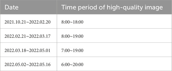
Table 1. Time periods for retaining high-quality images during different observation intervals.

Due to power outages and other issues, certain images are absent, resulting in a total of 2,400 images retained.

2.2 Meteorological data

Meteorological factors exhibit a significant correlation with PM_2.5 levels (Chen et al., 2020). In recent predictive models for PM_2.5, these factors have been utilized as auxiliary predictors, demonstrating their efficacy in forecasting fluctuations in PM_2.5 concentrations (Wen et al., 2019). In accordance with Zheng et al. (2021), TEM, relative humidity (RHU), and sea level pressure (PRS_Sea) have been identified as key meteorological auxiliary simulation factors. The meteorological data employed in this analysis consist of hourly observations from ground meteorological stations across China (http://data.cma.cn/site/index.html).

2.3 Pollutant concentration data

Pollutant concentration data were obtained from the real-time national urban air quality release platform of the China General Environmental Monitoring Station (https://air.cnemc.cn:18007). The hourly PM_2.5 mass concentration recorded at the nearest Railway Design Institute (RDI) site to Lanzhou University, where the images were captured, serves as the primary simulation target. Given the mobility of air and the processes of pollutant transmission and diffusion, the PM_2.5 concentrations at RDI exhibit a strong correlation with PM_2.5 concentrations at surrounding air quality monitoring sites (Chen et al., 2021). In this study, the hourly PM_2.5 concentration values monitored by other stations in Lanzhou City, excluding RDI, specifically the Education Bureau (EB), the Lanlian Hotel (LH), the Institute of Biological Products (IBP), and the Lanzhou University Campus of Yuzhong (LUCY), are selected as auxiliary simulation factors (Figure 1). The data corresponding to the times of image capture are utilized as the final pollutant concentration data.

Figure 1

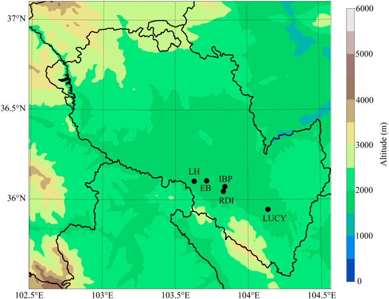
Figure 1. Distribution of air quality monitoring stations in Lanzhou.

2.4 Process of simulating PM_2.5 concentration

The primary research concepts of this article are illustrated in Figure 2. This study employed various CNN models for training using outdoor images, with the aim of identifying the optimal model based on evaluation metrics. The image features are extracted from the outputs of intermediate layers. Through importance analysis utilizing the RF algorithm (Breiman, 2001; Ji et al., 2023), image features exhibiting a significant correlation with PM_2.5 concentration are selected from the image feature vectors of zero less than 20%. These selected image features are then integrated with meteorological variables and pollutant concentration data for complete ensemble empirical mode decomposition with adaptive noise (CEEMDAN) signal decomposition (Jiang et al., 2021; Yang et al., 2022a; Yang et al., 2022b). An RF model is employed to train the low-frequency signal superimposed trend signal. Conversely, the high-frequency signals that yielded suboptimal training results with the RF model are subsequently analyzed using six additional machine learning models, from which the most effective regression model is selected for training the high-frequency signal. The post-training simulation results of the two frequency signals are combined to derive the final PM_2.5 concentration simulation.

Figure 2

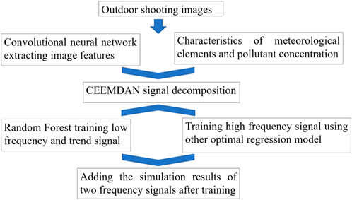
Figure 2. Workflow for PM_2.5 concentration simulation.

3 Hybrid machine learning to simulate PM_2.5 concentration

The model developed in this study is primarily divided into three stages to simulate PM_2.5 concentration in the region where outdoor images were captured in Lanzhou. The structure of the model is depicted in Figure 3.

Step 1. Preprocessing of image (Figure 3A): Within the training dataset, an image corresponding to the lowest PM_2.5 concentration, recorded at 10.00 μg/m³ at 15:00 on 7 November 2021, is designated as the background field image for clear weather conditions. To mitigate the impact of the background, the pixel values of the selected clear weather image are subtracted from the pixel values of all training images. Subsequently, these adjusted images are utilized for model training.

Step 2. Extraction of image features (Figure 3B): Utilizing outdoor image samples, the research employed a pre-trained network on image datasets characterized by a limited sample size through the transfer learning method (Jean et al., 2016). The earlier layers of the convolutional base are designed to encode more generic and reusable features, whereas the higher layers are responsible for encoding more specialized features (Chollet, 2017). This study implemented a fine-tuning approach to retrain the final layers of the pre-trained network model, thereby aligning the selected model more closely with the computer vision task of simulating PM_2.5 concentration using outdoor air quality images. This process facilitates the extraction of image features that exhibit a stronger correlation with PM_2.5 concentration for subsequent machine learning training in Step 3. The image data are paired with PM_2.5 concentration values and integrated into five deep learning models: VGG16 (Ahmed et al., 2022), VGG19 (Simonyan and Zisserman, 2014), ResNet50, ResNet101, and ResNet152. Through comparative analysis, ResNet50 was identified as the most effective pre-trained model for extracting image features. The levels of features can be enriched by the number of stacked layers (depth). However, network degradation may occur after the network is deepened by stacking, and the residual module of the ResNet algorithm can improve the depth of the neural network and solve the network degradation (He et al., 2016a). It is widely used in a variety of computer vision tasks (Li et al., 2022; Zheng et al., 2021). Figure 3B illustrates a partial structure of ResNet50 used in this study, and the upper layer of the original ResNet50 network is modified. Originally, the upper layers of the ResNet50 network consisted of a GlobalAveragePooling2D layer of size 2,048 and a dense layer of size 1,000 for dividing ImageNet images into 1,000 classes. To cater to the image regression task of simulating PM_2.5 concentration, after many experiments based on the original network structure of ResNet50, the last two layers are deleted, and new layers are added: First, a flattened layer of size 100,352 is added to one-dimensionalize the multi-dimensional input, so as to realize the transformation from the convolution layer to the dense layer. Second, five dense layers of size 256 are added through experiments. Then, a dropout layer is added to randomly discard neurons (and connections between neurons) from the neural network when the model works. The discarded neurons do not participate in forward and reverse propagation, and the structure of the neural network differs for each signal input. This technique reduces the complex co-adaptations of neurons and effectively prevents overfitting of the model (Krizhevsky et al., 2017; Srivastava et al., 2014). Then, a fully connected layer of size 64 is added as the middle layer of the deep network to extract the image feature vector. Finally, a dense layer and an activation layer of size 1 are added as the output layer of the ResNet network to output the simulated PM_2.5 concentration value. Because PM_2.5 concentration simulation is a regression task, the range of simulation is theoretically (−∞, +∞), so the activation layer uses a linear activation function. In the experiment, only the last five layers of the pre-trained ResNet50 are fine-tuned, and the bottom layers are “frozen” to ensure that their weights are always the weights of the original ResNet50 during the training process and will not be updated after training. Only the layers with parameters at the top of ResNet50 (Figure 3B) are trained, and the newly added layers are trained. These trained layers update the weights through the error backward passes between the simulated PM_2.5 concentration value and the observed value to optimize the model (He et al., 2016b). The experimental results show that the ResNet50 pre-trained model has a stronger simulation ability than the original model after fine-tuning.

Figure 3

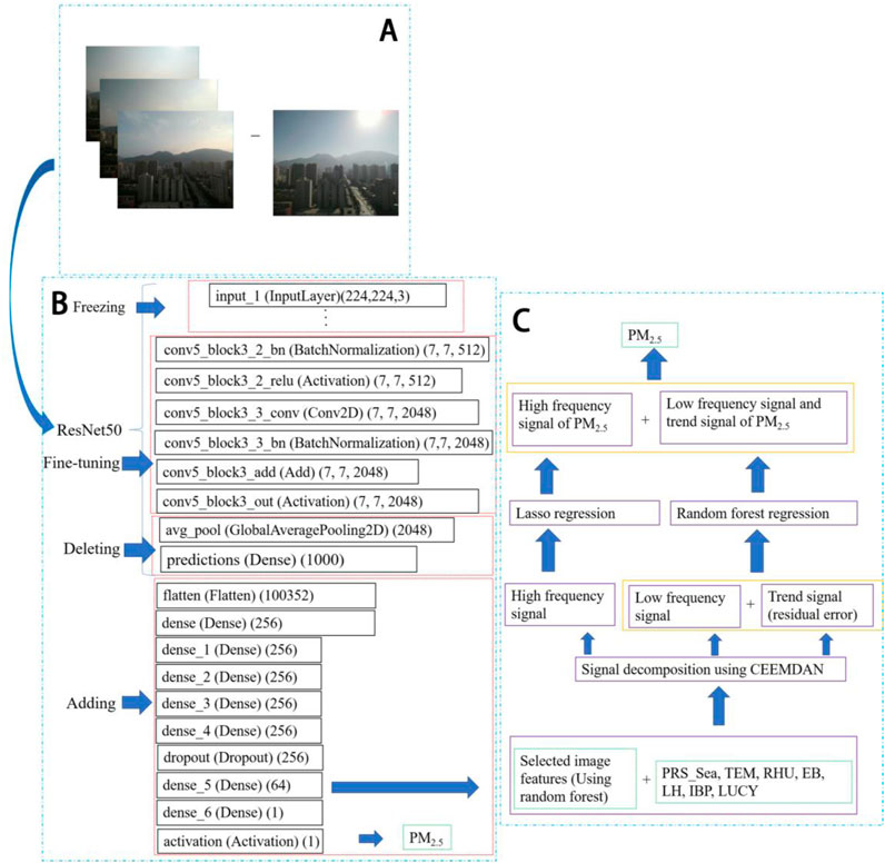
Figure 3. Hybrid machine learning model structure for PM_2.5 concentration simulation: (A) Step 1: Pixel values of the image with the lowest PM_2.5 concentration are subtracted from all input images; (B) Step 2: ResNet50 is selected after comparing five neural network models. GlobalAveragePooling2D and fully connected layers are replaced with custom layers. The last five layers are fine-tuned, while earlier layers remain frozen to optimize feature extraction; (C) Step 3: Extracted features are decomposed into high-frequency and low-frequency signals. These signals are trained using separate machine learning models, and their outputs are combined to generate the final PM_2.5 simulation.

After the completion of Step 1, prior to the integration of the images into the model training process, the image dimensions are standardized to 3 pixels × 224 pixels × 224 pixels. A total of 2,400 images are paired with their corresponding PM_2.5 concentration values at the relevant times, resulting in 2,400 data pairs. Among these, 1,600 pairs are designated for the training set, 400 pairs for the validation set, and 400 pairs for the test set. The network is trained to minimize the mean absolute error (MAE) and the mean squared error (MSE) between PM_2.5 concentrations predicted by the ResNet50 model and the observed values, utilizing the Adam optimization algorithm on mini-batches of the training samples (Kingma and Ba, 2014). The learning rate (lr) is set to 0.0001, while other parameters are maintained at their default values (${\beta }_1$ = 0.9, ${\beta }_2$ = 0.999, $\epsilon$ = 10^–8). The batch size is set at 5, and the total number of mini-batches in the training dataset is 320.

To enhance the image training set and optimize the model more effectively, data collection techniques are applied to the input images. These techniques include random horizontal and vertical flipping, as well as horizontal and vertical random translations, with the translation distance randomly varying between 0 and the maximum translation distance, which is defined as 10% of the image’s width or height. For the newly incorporated dense layer, the activation function is configured to use the rectified linear unit (ReLU) function. The ReLU activation function is advantageous as it does not suffer from gradient vanishing, and its sparse characteristics can significantly mitigate the issue of overfitting. Furthermore, the ReLU function is computationally simpler and faster than the sigmoid function (Xu et al., 2016). In the dropout layer that has been added, the dropout rate is set to 0.2. During the model training process, the number of epochs is established at 60, and the model is saved after each training iteration. The model that exhibits the lowest validation loss (val_loss) is selected for the extraction of 64 image feature vectors.

Step 3. Development of PM_2.5 concentration simulation (Figure 3C): A model is developed to simulate PM_2.5 concentration values utilizing image data, meteorological factors, and characteristics of pollutant concentration. In Figure 3C, not all of the 64 image feature vectors obtained in Step 2 are suitable for the subsequent PM_2.5 concentration simulation. Specifically, vectors containing a high proportion of 0 values are excluded, as their correlation with PM_2.5 concentrations is not significant. This lack of correlation is primarily due to the variability in PM_2.5 concentrations associated with identical 0 values in most instances. In this study, image feature vectors with 0 values exceeding 20% of the total are removed. The remaining vectors are then analyzed using an RF model to assess their importance. The image features corresponding to the three lowest importance scores are discarded, and the features that remain are utilized for PM_2.5 concentration simulation.

Experiments indicate that the accuracy of simulating PM_2.5 concentration using a single RF method is suboptimal. This study employs the signal decomposition technique (i.e., CEEMDAN) to decompose various features, including filtered image features, meteorological element features, pollutant concentration features, and the target value of PM_2.5 concentration. The decomposition yields high-frequency, low-frequency, and trend (residual) components, which are subsequently reconstructed into a high-frequency signal and a low-frequency signal superimposed with the trend. These two signals are then input into different machine learning models for simulation, and the results from both simulations are combined to produce the final simulation results. This approach aims to minimize errors associated with different frequency signals, thereby enhancing the accuracy of the final simulation results. The CEEMDAN method is an advanced algorithm derived from EEMD. It incorporates adaptive Gaussian white noise into the data decomposition process to mitigate pulse interference. In comparison to EEMD, CEEMDAN demonstrates superior completeness, eliminates reconstruction errors, offers faster computation speeds, and effectively reduces the number of intrinsic mode function (IMF) components that possess minimal significance and small amplitude (Torres et al., 2011).

For decomposed data, the signal of the IMF component is reconstructed utilizing continuous mean square error (CMSE) (Boudraa and Cexus, 2007; Zheng et al., 2018). It is assumed that ${\stackrel{\sim }{X}}_k\left(t\right)$ represents the outcome of reconstructing the kth IMF derived from CEEMDAN applied to the residual sequence using Equation 1:

${\stackrel{\sim }{X}}_k\left(t\right)={\displaystyle \sum _{i=k}^M}{IMF}_i\left(t\right)+R\left(t\right),k=1,2,\dots ,M,(1)$

where ${IMF}_i\left(t\right)$ is the ith IMF of CEEMDAN, and $R\left(t\right)$ is the residual sequence. The expression of CMSE is given as follows:

$CMSE\left({\stackrel{\sim }{X}}_k\left(t\right),{\stackrel{\sim }{X}}_{k+1}\left(t\right)\right)=\frac{1}{N}{\displaystyle \sum _{i=1}^N}{\left[{IMF}_k\left(t_i\right)\right]}^{2,}(2)$

where N is the number of samples sampled; $t_i$ is the time of sampling; and CMSE is the energy value of the kth IMF component. After calculating all CMSE using Equation 2, the minimum value is identified, which represents the optimal reconstruction coefficient for the low-frequency IMF. This coefficient serves as the demarcation between high-frequency and low-frequency IMF components. IMF components preceding the one associated with the minimum CMSE are classified as high-frequency components, while the remaining IMF components are categorized as low-frequency components.

If the minimum CMSE obtained through the aforementioned method corresponds to the energy value of the first IMF component, it becomes challenging to differentiate between high and low frequencies. In such instances, an alternative reconstruction algorithm is employed to effectively distinguish the high and low frequencies of IMF components (Qi et al., 2015). It is assumed that the signal is decomposed using CEEMDAN to yield M IMF components, and specific indicators ($A_1$… $A_M$) are established using Equations 3–5:

$A_1={IMF}_{1,}(3)$

$A_i={IMF}_1+{IMF}_2+\dots +{IMF}_i,(4)$

$A_M={IMF}_1+{IMF}_2+\dots +{IMF}_M,(5)$

The mean value of each index from $A_1$ to $A_M$ is calculated, and a t-test is conducted to determine whether the mean value is significantly different from 0. If a significant difference is observed between the mean value of $A_i$ and 0 for the first time, the components from ${IMF}_1$ to ${IMF}_{i-1}$ are classified as high-frequency components, while those from ${IMF}_i$ to ${IMF}_M$ are classified as low-frequency components. The high-frequency components are aggregated to produce the high-frequency signal, whereas the low-frequency components, along with the trend component, are combined to generate the low-frequency signal superimposed with the trend signal.

Different machine learning methods are employed to train signals of varying frequencies. A schematic diagram illustrating the process of signal decomposition and reconstruction is depicted in Figure 4, utilizing the image feature designated as 2 as a reference. The original dataset is decomposed into two components: a high-frequency signal and a low-frequency signal that is superimposed with a trend signal. These components are subsequently input into an RF model for independent training. The simulation results are then compared with the observed values from the validation set, utilizing metrics such as MAE, root mean square error (RMSE), and $R^2$. For signals that exhibited suboptimal simulation results with the RF model, alternative machine learning techniques were employed, including multiple regression (Han et al., 2020; Hu et al., 2023), support vector regression (SVR) (Luo et al., 2022; Smola and Scholkopf, 2004), K-nearest neighbors (KNN) (Shabani et al., 2020), bootstrap aggregating (Bagging) (Breiman, 1996), least absolute shrinkage and selection operator (Lasso) (Keeble et al., 2021; Tibshirani, 1996), and eXtreme gradient boosting (XGBoost) (Huang L. X. et al., 2021; Ma et al., 2020). Finally, an RF model was utilized to simulate the high-frequency signal, while a Lasso regression model was employed to simulate the low-frequency signal superimposed with the trend signal. The final simulation results were obtained by aggregating the outcomes from the two machine learning models.

Figure 4

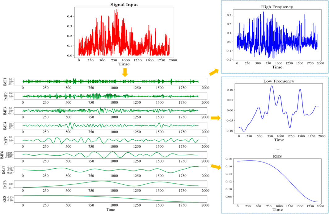
Figure 4. Schematic of signal decomposition and reconstruction for image feature signal 2 (Note: The decomposed components are categorized into high-frequency and low-frequency signals with a superimposed trend for further analysis).

Three indicators are employed to assess model performance: MAE, RMSE, and $R^2$. Equations 6–8 are provided for these three indicators:

$MAE=\frac{1}{N}{\displaystyle \sum _{i=1}^N}\left|x_i-{\widehat{x}}_i\right|,(6)$

$RMSE=\sqrt{\frac{1}{N}{\displaystyle \sum _{i=1}^N}{\left(x_i-{\widehat{x}}_i\right)}^2,}(7)$

$R^2=1-\frac{{\displaystyle \sum _{i=1}^N}{\left(x_i-{\widehat{x}}_i\right)}^2}{{\displaystyle \sum _{i=1}^N}{\left(x_i-\overline{x}\right)}^2,}(8)$

where $x_i$ is the ith observed value; ${\widehat{x}}_i$ is the ith simulated value; and $\overline{x}$ is the average of the observed value.

4 Results and discussion

4.1 Different model training

Two image recognition strategies are employed in this study. The first strategy involves deep learning applied to the original images, while the second strategy focuses on deep learning of the original images minus the clear weather image. Following the image preprocessing, five deep learning models are trained and evaluated for both strategies. Figure 5 illustrates the evaluation results derived from the validation set. Within the same model, the training conducted on images excluding the clear weather image yields superior simulation results than the training on the original images. Specifically, MAE and RMSE are relatively lower, and $R^2$ approaches 1. The visibility is indicated by the differences in pixel values between the two types of images. Higher PM_2.5 concentrations correlate with increased pollution levels and reduced visibility, which is represented in the images as increased blurriness and significant deviations in pixel values from those observed under clear weather conditions. Conversely, lower PM_2.5 concentrations result in minimal differences in pixel values. Through the process of image subtraction, the relationship between image information and PM_2.5 concentration is enhanced, thereby improving the accuracy of the simulation results. For the images that have undergone subtraction, training with the ResNet50 model yields the smallest MAE and RMSE values of 8.33 and 12.75, respectively, with an $R^2$ of 0.51. Consequently, the middle layer of the ResNet50 model is selected to extract 64 image features, which are numbered from 0 to 63.

Figure 5

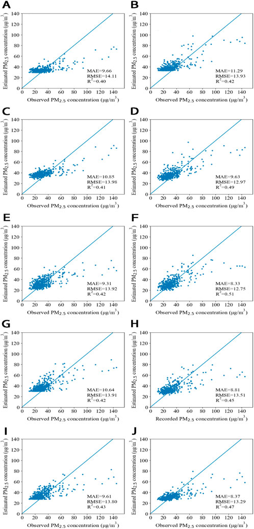
Figure 5. Comparison of the validation set performance before and after subtracting clear weather background image pixels using five deep learning models: (A) Original images with VGG16; (B) subtracted image with VGG16; (C) Original images with VGG19; (D) subtracted image with VGG19; (E) original images with ResNet50; (F) subtracted image with ResNet50; (G) original images with ResNet101; (H) subtracted image with ResNet101; (I) original images with ResNet152; (J) subtracted image with ResNet152.

4.2 Extracting features from images

In this experiment, a total of 64 image features were extracted. The image feature vectors corresponding to 1,600 training set images were paired with their respective PM_2.5 concentrations to create a new training dataset. Similarly, the image feature vectors for 400 validation set images were matched with the corresponding PM_2.5 concentrations to form a new validation dataset. First, a 3-fold cross-validation approach was employed. The ranges for the primary hyperparameters were established, and RandomizedSearchCV was utilized to optimize these hyperparameters within the RF framework (Bergstra and Bengio, 2012). Following the identification of an optimal set of hyperparameters from the defined range, both the training and validation datasets were input into the RF model utilizing the fine-tuned hyperparameters. Further refinement of the hyperparameters was conducted based on the MAE, RMSE, and $R^2$ between the simulated and observed PM_2.5 concentrations in the validation dataset. The final hyperparameter values determined through this process are outlined in Table 2.

Table 2

Table 2. Optimized hyperparameter selection results for RF model.

The significance of these image features was assessed following the training of the RF model utilizing the initially selected image features associated with PM_2.5 concentration. The results (Figure 6) indicate that among the 16 image features analyzed, the features corresponding to the three lowest importance scores (i.e., 16, 60, and 61) exhibited importance values of 0.015, 0.012, and 0.013, respectively. These values suggest a minimal correlation between these three features and PM_2.5 concentration. To enhance the model’s performance and improve the accuracy of the simulated PM_2.5 concentration, these features were excluded from subsequent analyses. Consequently, the remaining 13 image features were utilized in the final PM_2.5 concentration simulation.

Figure 6

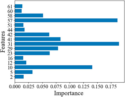
Figure 6. Importance of image features for PM_2.5 concentration simulation.

4.3 Signal decomposition and machine learning of its components

Different frequency signals employ various machine learning methods. The mass concentration of air pollutants exhibits periodicity across different scales, and signal decomposition enhances the predictive capability across these scales. Reconstruction is performed based on the CMSE values of each IMF component of the signal in Table 3. For instance, considering image feature 2, the CMSE value of IMF6 is the lowest, indicating that the optimal reconstruction coefficient for the low-frequency IMF is determined to be 6. This implies that the first five IMF components are classified as high-frequency components, which are reconstructed separately from the low-frequency components. All signals are reconstructed following this method. In Table 3, the optimal reconstruction coefficient for the low-frequency IMF of PRS_Sea and PM_2.5 concentration at the LH is 1, suggesting that the high-frequency component cannot be ascertained. Therefore, an alternative reconstruction algorithm is employed to differentiate between the high-frequency and low-frequency IMF components.

Table 3

Table 3. CMSE values for IMF components across all signals.

In Table 4, the mean value of Index 2 in PRS_Sea data is significantly different from 0 for the first time (P < 0.05). In this context, IMF1 corresponds to the high-frequency component, while IMF2, IMF3, IMF4, IMF5, IMF6, and IMF7 correspond to the low-frequency components. Additionally, the mean value of Index 6 in PM_2.5 concentration data from the LH is also significantly different from 0 for the first time. In this case, IMF1, IMF2, IMF3, IMF4, and IMF5 represent the high-frequency components, whereas IMF6 and IMF7 represent the low-frequency components. Similarly, IMFs of the same frequency components are aggregated to yield both high-frequency and low-frequency signals, respectively.

Table 4

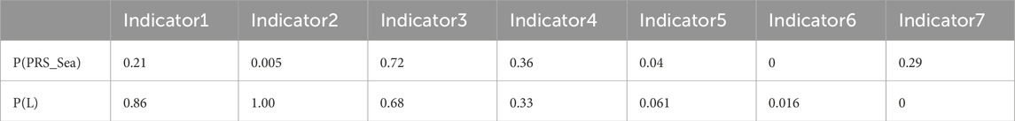
Table 4. P-value results of t-tests for all signal indicators (whether significantly different from 0).

The high-frequency signal and the low-frequency signal superimposed trend signal are utilized for training within the RF model. In Figure 7, the simulation results obtained from the RF model for the high-frequency signal of PM_2.5 concentration demonstrate relatively poor performance. While the model is capable of simulating the general trend of changes, it significantly underperforms in instances of abrupt increases in the high-frequency signal, yielding results that are considerably lower than the observed values. In contrast to the low-frequency signal, the high-frequency signal is characterized by a higher level of noise and instability in its variations. Furthermore, the simulation results produced by deep learning models tend to exhibit greater smoothness. As a result, the performance of the same model on the low-frequency signal, which exhibits more stable changes, is superior to that on the high-frequency signal. Additional machine learning models will be employed to train the high-frequency signal.

Figure 7

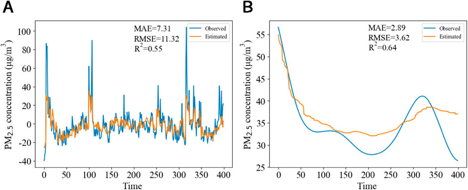
Figure 7. Validation set simulation results using RF on different frequency signals: (A) High-frequency signal; (B) low-frequency signal with superimposed trend.

The high-frequency signals were analyzed using six machine learning models. The simulation results of the high-frequency signals and the observed values from the validation set are illustrated in Figure 8. In this experiment, the Lasso regression model demonstrated the most effective training performance concerning the high-frequency signals. The MAE and RMSE between the simulated high-frequency signal results and the observed values of the validation set were the lowest, at 7.22 and 10.28, respectively, with an $R^2$ value of 0.63. The Lasso regression model employs compressed estimation, allowing for the construction of a more refined model through the implementation of a penalty function. It is a biased estimation that can achieve variable selection (Tibshirani, 1996), which improves the accuracy of high-frequency signal simulation of PM_2.5 concentration.

Figure 8

Figure 8. Validation set simulation results for high-frequency signals using different machine learning models: (A) Multiple regression; (B) Lasso; (C) Bagging; (D) SVR; (E) KNN; (F) XGBoost.

The main feature variables are important factors affecting machine learning results. According to the characteristic coefficient in the Lasso regression model to simulate the high-frequency signal of PM_2.5 concentration, and the characteristic importance in the random forest regression model is used to simulate the low-frequency signal superimposed trend signal of PM_2.5 concentration, as shown in Figure 9, in the Lasso regression, the characteristic variables that play an important role are sorted by coefficient: image feature 23, PM_2.5 concentration value of the Institute of Biological Products, temperature, PM_2.5 concentration value of the Lanlian Hotel, and PM_2.5 concentration value of the Education Bureau. The absolute values of the characteristic coefficients are 1.409, 0.380, 0.318, 0.066, and 0.002, respectively. In the random forest regression, the first five feature variables that play an important role are ranked by importance: image feature 5, image feature 23, PM_2.5 concentration of the Lanlian Hotel, image feature 29, and image feature 42, with importance values of 0.170, 0.137, 0.125, 0.084 and 0.080, respectively. Experimental results indicate that image features, meteorological elements, and pollutant concentration features are most influential in the Lasso regression model for high-frequency signal simulation, whereas image features and pollutant concentration features play a more critical role in the RF model for the low-frequency signal superimposed trend signal.

Figure 9

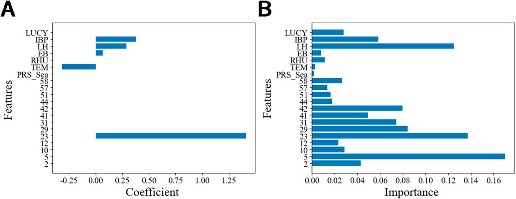
Figure 9. Feature contributions in Lasso and RF models for PM_2.5 simulation: (A) Characteristic coefficients in Lasso regression for high-frequency signals; (B) feature importance in RF regression for low-frequency signals superimposed trend signal.

Figure 10 shows that the incorporation of high-frequency signals into the Lasso regression model, along with the integration of low-frequency superimposed trend signals into the RF model, has significantly enhanced the simulation capabilities of the validation set when compared to the performance of a single RF model. This improvement is particularly notable in the simulation of both low and high concentrations of PM_2.5. The training utilizing split-frequency methods demonstrates superior simulation performance. Specifically, the MAE and RMSE between the simulated PM_2.5 concentrations and the observed values from the corresponding validation set have decreased by 1.05 and 1.59, respectively. Furthermore, $R^2$ increased from 0.59 to 0.70.

Figure 10

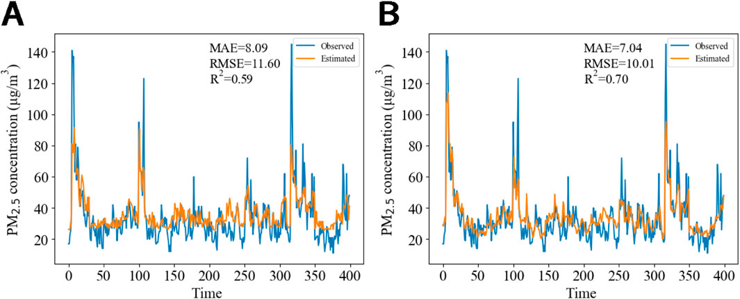
Figure 10. Comparison of simulation results for the validation set using original and split-frequency signals: (A) results with the original signal in a machine learning model; (B) combined results of split-frequency signals using different models.

The effects of two experiments on the simulation of different concentrations of PM_2.5 in the validation set are analyzed. Figure 11 shows the error comparison of the validation set simulation after the original signal is brought into the random forest model (Figure 11A) and the split-frequency signal is brought into different models (Figure 11B). The PM_2.5 concentration value less than or equal to 75 μg/m³ is recorded as the low value, and the PM_2.5 concentration value greater than 75 μg/m³ is recorded as the high value. The mean value of the absolute value of the error of the simulation of low PM_2.5 concentration in the validation set after the split-frequency signal was brought into different models was 7.22 μg/m³, which was slightly smaller than the mean value of the absolute value of the error of the simulation of low PM_2.5 concentration after the original signal was brought into the random forest model (8.35 μg/m³). The mean value of the absolute error of the simulation of high PM_2.5 concentration in the validation set after the split-frequency signal is brought into different models is 26.57 μg/m³, which is much smaller than the mean value of the absolute error of the simulation of high PM_2.5 concentration after the original signal is brought into the random forest model (36.08 μg/m³). It can be seen that the simulation effect of the split-frequency signal brought into different models for high PM_2.5 concentration is much stronger than that of the original signal brought into the random forest model, which further indicates that the split-frequency signal brought into different models can improve the simulation ability of the validation set.

Figure 11

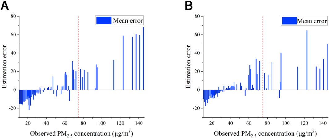
Figure 11. Validation set simulation errors for original and split-frequency signal models: (A) errors from the original signal simulation using the RF model; (B) errors from split-frequency signal simulation using different models. (The error is calculated as the difference between the observed and simulated values, with errors averaged for cases where the observed PM_2.5 concentration value is repeated).

4.4 Analysis of simulation for the test set

The evaluation results for the test set (Figure 12) indicate that the Lasso regression model provides a more accurate simulation of the high-frequency signal of PM_2.5 concentration than other models. In Figure 12A, Lasso regression effectively captures the trend of the high-frequency signal, including its abrupt increases. Although the MAE and RMSE values are higher than those of the validation set, $R^2$ is 0.74, which is closer to 1, suggesting a strong relationship between the simulated and observed values. In Figure 12B, the RF model exhibits slightly reduced efficacy in simulating the low-frequency signal superimposed trend signal of PM_2.5 mass concentration within the test set. However, it does provide a reasonable approximation of the overall trend. Notably, in instances where the Lasso regression model’s simulated values for the high-frequency signal exceed the observed values (e.g., during time points 0–50 and around time point 100), the RF model tends to underestimate the simulated values of the low-frequency signal superimposed trend signal. Conversely, during periods when the Lasso regression model’s simulated values for the high-frequency signals are lower than the observed values (e.g., during time points 150–250), the RF model’s simulated values for the low-frequency signal superimposed trend signal are higher than the observed values. In Figure 12C, the PM_2.5 concentration simulation is satisfactory, with an $R^2$ of 0.83 between the simulated PM_2.5 concentration and the observed values in the test set, indicating the superior simulation performance of the model.

Figure 12

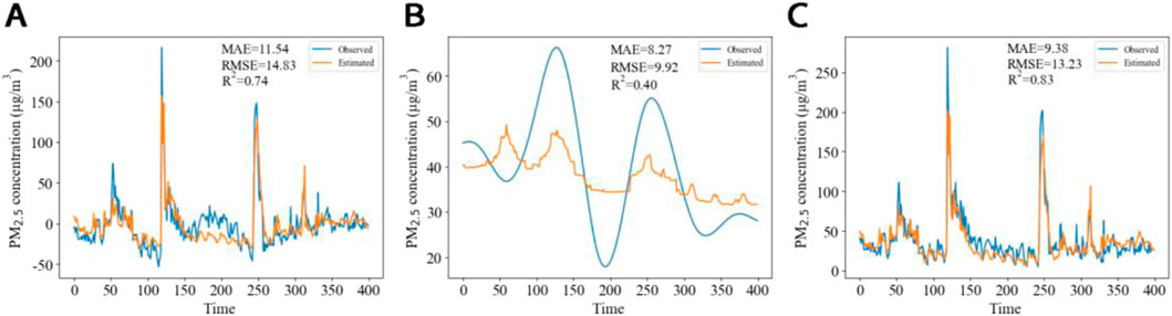
Figure 12. Test set performance of the Lasso and RF models for PM_2.5 concentration simulation: (A) high-frequency signal simulation using Lasso regression; (B) low-frequency signal superimposed trend signal simulation using RF regression; (C) combined simulation versus observed values.

4.5 Discussion

In this study, the image features are extracted by ResNet50 and selected by random forest importance analysis, and the PM_2.5 concentration of the locations photographed in Lanzhou City is simulated by using CEEMDAN for signal frequency division and reconstruction and combining random forest and Lasso regression based on the image features, meteorological element features, and pollutant concentration features. Finally, the hybrid machine learning model of Resnet50, random forest, and Lasso was established, and the model achieved satisfactory results on the verification set and the test set. The model demonstrated satisfactory performance on both the validation and test datasets. This approach has practical implications for PM_2.5 monitoring; in instances where air quality monitoring stations are in close proximity, PM_2.5 monitoring instruments at certain stations could be substituted with camera equipment. The images captured could then be processed through the hybrid machine learning model to estimate PM_2.5 concentrations, thereby significantly reducing monitoring costs. However, due to the small accumulation of images, the model still has the problem of overfitting, and the collection of environmental images is relatively single, so we need to collect images for a longer period of time or try new and different machine learning methods or other advanced state-of-the-art models to make the simulation results more accurate. We also need to collect outdoor images of different scenes to further verify the generalization ability of the model.

5 Conclusion

In recent decades, air pollution has posed a serious threat to human health and has raised significant public concern. Developing efficient and low-cost pollutant concentration simulation methods is essential for safeguarding human health and improving air pollution control strategies. This article proposes a more accurate hybrid model combining ResNet50, RF, and Lasso regression to simulate PM_2.5 concentrations using 2,400 outdoor air quality images captured in Lanzhou City from 15:00 on 21 October 2021 to 13:00 on 16 May 2022, along with corresponding meteorological and pollutant concentration data. The main conclusions are as follows:

The results from the three evaluation metrics show that, for the same CNN model, simulation results are improved when the clear-weather pixel values are subtracted from the original images. Among the five CNN models tested, ResNet50 consistently yielded the best training results, as evidenced by the MAE, RMSE, and $R^2$ values. Therefore, ResNet50 was chosen for feature extraction from the images.

Random forest is used to train the low-frequency signal superimposed trend signals of PM_2.5 concentration. The high-frequency signal, which showed poorer training performance using RF, was further analyzed with six machine learning models. The Lasso regression model was selected to train the high-frequency signal based on a comparison of simulation results against observed PM_2.5 concentrations. The hybrid model, combining RF for the low-frequency signal superimposed trend signal and Lasso regression for the high-frequency signal, demonstrated superior performance compared to using RF alone.

In the Lasso regression model for the high-frequency signal, image features, meteorological elements, and PM_2.5 concentration data were found to play a more significant role. Conversely, for an RF model applied to the low-frequency signal superimposed trend signal, image features and pollutant concentration data were more influential. The Lasso regression model more accurately simulated high-frequency signal variations and sudden increases in PM_2.5 concentration. Meanwhile, the RF model simulated the low-frequency signal superimposed trend signal of PM_2.5 concentration in the test set slightly less well, but it could roughly simulate the overall change trend. The combination of these models resulted in a more accurate overall simulation.

The final comparison between the summed values of both simulations and the observed PM_2.5 concentrations revealed that the hybrid model consistently produced more accurate results. This demonstrates that the hybrid approach outperforms individual models in simulating PM_2.5 concentrations. Furthermore, the hybrid model offers a rapid, reliable, and cost-effective method for estimating air pollution. The results highlight the practical value of using image features to provide precise and reliable air quality measurements, with important implications for the management and monitoring of air pollution.

Data availability statement

The raw data supporting the conclusions of this article will be made available by the authors, without undue reservation.

Author contributions

MM: conceptualization, data curation, funding acquisition, methodology, project administration, supervision, validation, writing–original draft, and writing–review and editing. ZZ: formal analysis, investigation, visualization, and writing–original draft. YM: formal analysis, methodology, supervision, and writing–review and editing. YC: investigation and writing–review and editing. GK: formal analysis and writing–review and editing.

Funding

The author(s) declare that financial support was received for the research, authorship, and/or publication of this article. This research was supported by the Drought Meteorological Science Research Fund Project (Grant No. IAM202002).

Acknowledgments

The authors express their sincere gratitude to the Supercomputing Center of Lanzhou University for providing essential computational resources and to the National Meteorological Information Center for supplying the meteorological data used in this study. Appreciation is also extended to the data.epmap.org platform for facilitating access to critical research data. The authors are deeply thankful to the reviewers for their valuable comments and suggestions, which significantly enhanced the quality of this work.

Conflict of interest

The authors declare that the research was conducted in the absence of any commercial or financial relationships that could be construed as a potential conflict of interest.

Generative AI statement

The authors declare that no Generative AI was used in the creation of this manuscript.

Publisher’s note

All claims expressed in this article are solely those of the authors and do not necessarily represent those of their affiliated organizations, or those of the publisher, the editors and the reviewers. Any product that may be evaluated in this article, or claim that may be made by its manufacturer, is not guaranteed or endorsed by the publisher.

References

Ahmed, M., Shen, Y. L., Ahmed, M., Xiao, Z. M., Cheng, P., Ali, N., et al. (2022). AQE-net: a deep learning model for estimating air quality of karachi city from mobile images. Remote Sens. 14 (22), 5732. doi:10.3390/rs14225732

CrossRef Full Text | Google Scholar

Bai, Y., Zeng, B., Li, C., and Zhang, J. (2019). An ensemble long short-term memory neural network for hourly PM_2.5 concentration forecasting. Chemosphere 222, 286–294. doi:10.1016/j.chemosphere.2019.01.121

PubMed Abstract | CrossRef Full Text | Google Scholar

Beloconi, A., Kamarianakis, Y., and Chrysoulakis, N. (2016). Estimating urban PM₁₀ and PM_2.5 concentrations, based on synergistic MERIS/AATSR aerosol observations, land cover and morphology data. Remote Sens. Environ. 172, 148–164. doi:10.1016/j.rse.2015.10.017

CrossRef Full Text | Google Scholar

Bergstra, J., and Bengio, Y. (2012). Random search for hyper-parameter optimization. J. Mach. Learn. Res. 13, 281–305.

Google Scholar

Boudraa, A. O., and Cexus, J. C. (2007). EMD-Based signal filtering. IEEE Trans. Instrum. Meas. 56 (6), 2196–2202. doi:10.1109/tim.2007.907967

CrossRef Full Text | Google Scholar

Brauer, M., Freedman, G., Frostad, J., van Donkelaar, A., Martin, R. V., Dentener, F., et al. (2016). Ambient air pollution exposure estimation for the global burden of disease 2013. Environ. Sci. Technol. 50 (1), 79–88. doi:10.1021/acs.est.5b03709

PubMed Abstract | CrossRef Full Text | Google Scholar

Breiman, L. (1996). Bagging predictors. Mach. Learn. 24 (2), 123–140. doi:10.1007/bf00058655

CrossRef Full Text | Google Scholar

Breiman, L. (2001). Random forests. Mach. Learn. 45 (1), 5–32. doi:10.1023/a:1010933404324

CrossRef Full Text | Google Scholar

Brook, R. D., Rajagopalan, S., Pope, C. A., Brook, J. R., Bhatnagar, A., Diez-Roux, A. V., et al. (2010). Particulate matter air pollution and cardiovascular disease an update to the scientific statement from the American heart association. Circulation 121 (21), 2331–2378. doi:10.1161/CIR.0b013e3181dbece1

PubMed Abstract | CrossRef Full Text | Google Scholar

Carvalho, H. (2016). The air we breathe: differentials in global air quality monitoring. Lancet Respir. Med. 4 (8), 603–605. doi:10.1016/s2213-2600(16)30180-1

PubMed Abstract | CrossRef Full Text | Google Scholar

Chen, Y., Ma, M. J., Su, Y. M., and Huang, W. L. (2021). A study on the differences of PM_2.5 distribution between major cities and their background areas in the Beijing-Tianjin-Hebei region. J. Lanzhou Univ. Nat. Sci. 57 (04), 559–568. doi:10.13885/j.issn.0455-2059.2021.04.017

CrossRef Full Text | Google Scholar

Chen, Z. Y., Chen, D. L., Zhao, C. F., Kwan, M. P., Cai, J., Zhuang, Y., et al. (2020). Influence of meteorological conditions on PM_2.5 concentrations across China: a review of methodology and mechanism. Environ. Int. 139, 105558. doi:10.1016/j.envint.2020.105558

PubMed Abstract | CrossRef Full Text | Google Scholar

Chollet, F. (2017). Deep learning with Python. United States: Manning Publications Co. Available at: https://forums.manning.com/forums/deep-learning-with-python.

Google Scholar

Du, P., Wang, J. Z., Hao, Y., Niu, T., and Yang, W. D. (2020). A novel hybrid model based on multi-objective Harris hawks optimization algorithm for daily PM_2.5 and PM₁₀ forecasting. Appl. Soft Comput. 96, 106620. doi:10.1016/j.asoc.2020.106620

CrossRef Full Text | Google Scholar

Fang, X., Zou, B., Liu, X. P., Sternberg, T., and Zhai, L. (2016). Satellite-based ground PM_2.5 estimation using timely structure adaptive modeling. Remote Sens. Environ. 186, 152–163. doi:10.1016/j.rse.2016.08.027

CrossRef Full Text | Google Scholar

Geng, G. N., Zhang, Q., Martin, R. V., van Donkelaar, A., Huo, H., Che, H. Z., et al. (2015). Estimating long-term PM_2.5 concentrations in China using satellite-based aerosol optical depth and a chemical transport model. Remote Sens. Environ. 166, 262–270. doi:10.1016/j.rse.2015.05.016

CrossRef Full Text | Google Scholar

Han, H., Liu, J. E., Shu, L., Wang, T. J., and Yuan, H. L. (2020). Local and synoptic meteorological influences on daily variability in summertime surface ozone in eastern China. Atmos. Chem. Phys. 20 (1), 203–222. doi:10.5194/acp-20-203-2020

CrossRef Full Text | Google Scholar

Hayes, R. B., Lim, C., Zhang, Y. L., Cromar, K., Shao, Y. Z., Reynolds, H. R., et al. (2020). PM_2.5 air pollution and cause-specific cardiovascular disease mortality. Int. J. Epidemiol. 49 (1), 25–35. doi:10.1093/ije/dyz114

PubMed Abstract | CrossRef Full Text | Google Scholar

He, K. M., Zhang, X. Y., Ren, S. Q., and Sun, J. (2016a). “Deep residual learning for image recognition,” in 2016 IEEE Conference on Computer Vision and Pattern Recognition (CVPR), Las Vegas, NV, USA, 27-30 June 2016, 770–778. doi:10.1109/cvpr.2016.90

CrossRef Full Text | Google Scholar

He, K. M., Zhang, X. Y., Ren, S. Q., and Sun, J. (2016b). Identity mappings in deep residual networks. 14th Eur. Conf. Comput. Vis. (ECCV) 9908, 630–645. doi:10.1007/978-3-319-46493-0_38

CrossRef Full Text | Google Scholar

Hu, C. G., Huang, G. L., and Wang, Z. Y. (2023). Exploring the seasonal relationship between spatial and temporal features of land surface temperature and its potential drivers: the case of Chengdu metropolitan area, China. Front. Earth Sci. 11. doi:10.3389/feart.2023.1226795

CrossRef Full Text | Google Scholar

Hu, X. F., Waller, L. A., Lyapustin, A., Wang, Y. J., Al-Hamdan, M. Z., Crosson, W. L., et al. (2014). Estimating ground-level PM_2.5 concentrations in the Southeastern United States using MAIAC AOD retrievals and a two-stage model. Remote Sens. Environ. 140, 220–232. doi:10.1016/j.rse.2013.08.032

CrossRef Full Text | Google Scholar

Huang, G. Y., Li, X. Y., Zhang, B., and Ren, J. D. (2021a). PM_2.5 concentration forecasting at surface monitoring sites using GRU neural network based on empirical mode decomposition. Sci. Total Environ. 768, 144516. doi:10.1016/j.scitotenv.2020.144516

PubMed Abstract | CrossRef Full Text | Google Scholar

Huang, L. X., Kang, J. F., Wan, M. X., Fang, L., Zhang, C. Y., and Zeng, Z. L. (2021b). Solar radiation prediction using different machine learning algorithms and implications for extreme climate events. Front. Earth Sci. 9. doi:10.3389/feart.2021.596860

CrossRef Full Text | Google Scholar

Jean, N., Burke, M., Xie, M., Davis, W. M., Lobell, D. B., and Ermon, S. (2016). Combining satellite imagery and machine learning to predict poverty. Science 353 (6301), 790–794. doi:10.1126/science.aaf7894

PubMed Abstract | CrossRef Full Text | Google Scholar

Ji, Y., Zhi, X. F., Wu, Y., Zhang, Y. Q., Yang, Y. T., Peng, T., et al. (2023). Regression analysis of air pollution and pediatric respiratory diseases based on interpretable machine learning. Front. Earth Sci. 11. doi:10.3389/feart.2023.1105140

CrossRef Full Text | Google Scholar

Jiang, F. X., Zhang, C. Y., Sun, S. L., and Sun, J. Y. (2021). Forecasting hourly PM_2.5 based on deep temporal convolutional neural network and decomposition method. Appl. Soft Comput. 113, 107988. doi:10.1016/j.asoc.2021.107988

CrossRef Full Text | Google Scholar

Keeble, J., Yiu, Y. Y. S., Archibald, A. T., O'Connor, F., Sellar, A., Walton, J., et al. (2021). Using machine learning to make computationally inexpensive projections of 21st century stratospheric column ozone changes in the tropics. Front. Earth Sci. 8. doi:10.3389/feart.2020.592667

CrossRef Full Text | Google Scholar

Kingma, D. P., and Ba, J. L. (2014). “Adam: a method for stochastic optimization,” in the 3rd International Conference for Learning Representations, Banff, Canada, Apr 14 - 16, 2014, 1–15. doi:10.48550/arXiv.1412.6980

CrossRef Full Text | Google Scholar

Krizhevsky, A., Sutskever, I., and Hinton, G. E. (2017). ImageNet classification with deep convolutional neural networks. Commun. ACM. 60 (6), 84–90. doi:10.1145/3065386

CrossRef Full Text | Google Scholar

Leiva, M. A., Santibanez, D. A., Ibarra, S., Matus, P., and Seguel, R. (2013). A five-year study of particulate matter (PM_2.5) and cerebrovascular diseases. Environ. Pollut. 181, 1–6. doi:10.1016/j.envpol.2013.05.057

PubMed Abstract | CrossRef Full Text | Google Scholar

Li, K., Ma, Z. G., Xu, L. L., Chen, Y., Ma, Y. Y., Wu, W., et al. (2022). Depthwise separable ResNet in the MAP framework for hyperspectral image classification. IEEE Geosci. Remote Sens. Lett. 19, 1–5. doi:10.1109/lgrs.2020.3033149

CrossRef Full Text | Google Scholar

Li, X., Peng, L., Yao, X. J., Cui, S. L., Hu, Y., You, C. Z., et al. (2017). Long short-term memory neural network for air pollutant concentration predictions: method development and evaluation. Environ. Pollut. 231, 997–1004. doi:10.1016/j.envpol.2017.08.114

PubMed Abstract | CrossRef Full Text | Google Scholar

Liaw, J. J., Huang, Y. F., Hsieh, C. H., Lin, D. C., and Luo, C. H. (2020). PM_2.5 concentration estimation based on image processing schemes and simple linear regression. Sensors 20 (8), 2423. doi:10.3390/s20082423

PubMed Abstract | CrossRef Full Text | Google Scholar

Liu, H., Duan, Z., and Chen, C. (2020). A hybrid multi-resolution multi-objective ensemble model and its application for forecasting of daily PM_2.5 concentrations. Inf. Sci. 516, 266–292. doi:10.1016/j.ins.2019.12.054

CrossRef Full Text | Google Scholar

Liu, H., Jin, K. R., and Duan, Z. (2019). Air PM_2.5 concentration multi-step forecasting using a new hybrid modeling method: comparing cases for four cities in China. Atmos. Pollut. Res. 10 (5), 1588–1600. doi:10.1016/j.apr.2019.05.007

CrossRef Full Text | Google Scholar

Liu, H., Yu, Y., Ma, X. Y., Liu, X. Y., Dong, L. X., and Xia, D. S. (2023). Monitoring the impact of the COVID-19 lockdown on air quality in Lanzhou: implications for future control strategies. Front. Earth Sci. 10. doi:10.3389/feart.2022.1011536

CrossRef Full Text | Google Scholar

Luo, S. X., Zhang, M. L., Nie, Y. M., Jia, X. A., Cao, R. H., Zhu, M. T., et al. (2022). Forecasting of monthly precipitation based on ensemble empirical mode decomposition and Bayesian model averaging. Front. Earth Sci. 10. doi:10.3389/feart.2022.926067

PubMed Abstract | CrossRef Full Text | Google Scholar

Luo, Z. Y., Huang, F. F., and Liu, H. (2020). PM_2.5 concentration estimation using convolutional neural network and gradient boosting machine. J. Environ. Sci. 98, 85–93. doi:10.1016/j.jes.2020.04.042

PubMed Abstract | CrossRef Full Text | Google Scholar

Ma, J. H., Yu, Z. Q., Qu, Y. H., Xu, J. M., and Cao, Y. (2020). Application of the XGBoost machine learning method in PM_2.5 prediction: a case study of Shanghai. Aerosol Air Qual. Res. 20 (1), 128–138. doi:10.4209/aaqr.2019.08.0408

CrossRef Full Text | Google Scholar

Ma, S., Li, Z. Q., Chen, H., Liu, H., Yang, F., Zhou, Q., et al. (2019). Analysis of air quality characteristics and sources of pollution during heating period in Lanzhou. Environ. Chem. 38 (02), 344–353. doi:10.7524/j.issn.0254-6108.2018083103

CrossRef Full Text | Google Scholar

Pascal, M., Falq, G., Wagner, V., Chatignoux, E., Corso, M., Blanchard, M., et al. (2014). Short-term impacts of particulate matter (PM₁₀, PM_10-2.5, PM_2.5) on mortality in nine French cities. Atmos. Environ. 95, 175–184. doi:10.1016/j.atmosenv.2014.06.030

CrossRef Full Text | Google Scholar

Qi, S. Z., Zhao, X., and Tan, X. J. (2015). A study on the formation mechanism of Chinese carbon market price based on EEMD model. Wuhan Univ. Journal Philosophy and Soc. Sci. 68 (04), 56–65. doi:10.14086/j.cnki.wujss.2015.04.008

CrossRef Full Text | Google Scholar

Shabani, S., Samadianfard, S., Sattari, M. T., Mosavi, A., Shamshirband, S., Kmet, T., et al. (2020). Modeling Pan evaporation using Gaussian process regression K-nearest Neighbors random forest and support vector machines; comparative analysis. Atmosphere 11 (1), 66. doi:10.3390/atmos11010066

CrossRef Full Text | Google Scholar

Simonyan, K., and Zisserman, A. (2014). Very deep convolutional networks for large-scale image recognition. Comput. Sci., 1–14. doi:10.48550/arXiv.1409.1556

CrossRef Full Text | Google Scholar

Smola, A. J., and Scholkopf, B. (2004). A tutorial on support vector regression. Statistics Comput. 14 (3), 199–222. doi:10.1023/b:Stco.0000035301.49549.88

CrossRef Full Text | Google Scholar

Srivastava, N., Hinton, G., Krizhevsky, A., Sutskever, I., and Salakhutdinov, R. (2014). Dropout: a simple way to prevent neural networks from overfitting. J. Mach. Learn. Res. 15, 1929–1958. doi:10.5555/2627435.2670313

CrossRef Full Text | Google Scholar

Sun, W., and Li, Z. Q. (2020). Hourly PM_2.5 concentration forecasting based on feature extraction and stacking-driven ensemble model for the winter of the Beijing-Tianjin-Hebei area. Atmos. Pollut. Res. 11 (6), 110–121. doi:10.1016/j.apr.2020.02.022

CrossRef Full Text | Google Scholar

Tibshirani, R. (1996). Regression shrinkage and selection via the Lasso. J. R. Stat. Soc. Ser. B-Methodological. 58 (1), 267–288. doi:10.1111/j.2517-6161.1996.tb02080.x

CrossRef Full Text | Google Scholar

Torres, M. E., Colominas, M. A., Schlotthauer, G., and Flandrin, P. (2011). “A complete ensemble empirical mode decomposition with adaptive noise,” in IEEE International Conference on Acoustics, Speech, and Signal Processing (ICASSP), Prague, Czech Republic, 22-27 May 2011, 4144–4147. doi:10.1109/ICASSP.2011.5947265

CrossRef Full Text | Google Scholar

Wang, D. Y., Wei, S., Luo, H. Y., Yue, C. Q., and Grunder, O. (2017). A novel hybrid model for air quality index forecasting based on two-phase decomposition technique and modified extreme learning machine. Sci. Total Environ. 580, 719–733. doi:10.1016/j.scitotenv.2016.12.018

PubMed Abstract | CrossRef Full Text | Google Scholar

Wang, F. L., Li, Z. Q., Wang, F. T., You, X. N., Xia, D. S., Zhang, X., et al. (2021). Air pollution in a low-industry city in China's silk road economic belt: characteristics and potential sources. Front. Earth Sci. 9. doi:10.3389/feart.2021.527475

CrossRef Full Text | Google Scholar

Wang, J. L., Zhang, Y. H., Shao, M., Liu, X. L., Zeng, L. M., Cheng, C. L., et al. (2006). Quantitative relationship between visibility and mass concentration of PM_2.5 in Beijing. J. Environ. Sci. 18 (3), 475–481. Available at: https://pubmed.ncbi.nlm.nih.gov/17294643/.

PubMed Abstract | Google Scholar

Wang, X. C., Wang, M. Z., Liu, X. J., Mao, Y., Chen, Y., and Dai, S. S. (2024). Surveillance-image-based outdoor air quality monitoring. Environ. Sci. Ecotechnol. 18, 100319. doi:10.1016/j.ese.2023.100319

PubMed Abstract | CrossRef Full Text | Google Scholar

Wang, X. M., Tian, G. H., Yang, D. Y., Zhang, W. X., Lu, D. B., and Liu, Z. M. (2018). Responses of PM_2.5 pollution to urbanization in China. Energy Policy 123, 602–610. doi:10.1016/j.enpol.2018.09.001

CrossRef Full Text | Google Scholar

Wen, C. C., Liu, S., Yao, X. J., Peng, L., Li, X., Hu, Y., et al. (2019). A novel spatiotemporal convolutional long short-term neural network for air pollution prediction. Sci. Total Environ. 654, 1091–1099. doi:10.1016/j.scitotenv.2018.11.086

PubMed Abstract | CrossRef Full Text | Google Scholar

Wilson, B., Pope, M., Melecio-Vazquez, D., Hsieh, H., Alfaro, M., Shu, E., et al. (2024). Climate adjusted projections of the distribution and frequency of poor air quality days for the contiguous United States. Front. Earth Sci. 12. doi:10.3389/feart.2024.1320170

CrossRef Full Text | Google Scholar

Xu, L., Choy, C. S., and Li, Y. W. (2016). “Deep sparse rectifier neural networks for speech denoising,” in 15th International Workshop on Acoustic Signal Enhancement (IWAENC), Xi'an, China, 13-16 September 2016, 1–5. doi:10.1109/IWAENC.2016.7602891

CrossRef Full Text | Google Scholar

Yang, H., Liu, Z. H., and Li, G. H. (2022a). A new hybrid optimization prediction model for PM_2.5 concentration considering other air pollutants and meteorological conditions. Chemosphere 307, 135798. doi:10.1016/j.chemosphere.2022.135798

PubMed Abstract | CrossRef Full Text | Google Scholar

Yang, H., Zhao, J. L., and Li, G. H. (2022b). A new hybrid prediction model of PM_2.5 concentration based on secondary decomposition and optimized extreme learning machine. Environ. Sci. Pollut. Res. 29 (44), 67214–67241. doi:10.1007/s11356-022-20375-y

PubMed Abstract | CrossRef Full Text | Google Scholar

Yang, H. F., Zhu, Z. J., Li, C., and Li, R. R. (2020a). A novel combined forecasting system for air pollutants concentration based on fuzzy theory and optimization of aggregation weight. Appl. Soft Comput. 87, 105972. doi:10.1016/j.asoc.2019.105972

CrossRef Full Text | Google Scholar

Yang, Y. P., Wang, L. N., Yang, L. L., Tao, H. H., and Jiang, L. (2020b). Air pollution characteristics and potential sources in Lanzhou during dust weather. J. Desert Res. 40 (03), 60–66. doi:10.7522/j.issn.1000-694X.2019.00045

CrossRef Full Text | Google Scholar

Zheng, H. M., Peng, D. D., Gu, S. M., Zheng, Y., and Chen, K. (2018). Research on drill pulse signal extraction algorithm based on CMSE. J. Electron. Meas. Instrum. 32 (03), 170–176. doi:10.13382/j.jemi.2018.03.024

CrossRef Full Text | Google Scholar

Zheng, T. S., Bergin, M., Wang, G. Y., and Carlson, D. (2021). Local PM_2.5 hotspot detector at 300 m resolution: a random forest-convolutional neural network joint model jointly trained on satellite images and meteorology. Remote Sens. 13 (7), 1356. doi:10.3390/rs13071356

CrossRef Full Text | Google Scholar

Zheng, T. S., Bergin, M. H., Hu, S. J., Miller, J., and Carlson, D. E. (2020). Estimating ground-level PM_2.5 using micro-satellite images by a convolutional neural network and random forest approach. Atmos. Environ. 230, 117451. doi:10.1016/j.atmosenv.2020.117451

CrossRef Full Text | Google Scholar

Zhong, L. J., Zheng, J. Y., Lei, G. Q., and Chen, J. (2007). Quantitative uncertainty analysis in air pollutant emission inventories: methodology and case study. Res. Environ. Sci. (04), 15–20. doi:10.13198/j.res.2007.04.19.zhonglj.004

CrossRef Full Text | Google Scholar

Zhu, R., Zhang, G. Z., and Xie, H. G. (2006). Analysis of the cause of Lanzhou air pollution. J. Lanzhou Jiaot. Univ. Nat. Sci. (04), 59–62.

Google Scholar