An early warning system for oil wells based on improved long short-term memory network

Timely and accurate oil well production warnings are crucial for optimizing oilfield management and enhancing economic returns. Traditional methods for predicting oil well production and early warning systems face significant limitations in terms of adaptability and accuracy. Artificial intelligence offers an effective solution to address these challenges. This study focuses on the ultra-high water cut stage in water-driven medium-to-high permeability reservoirs, where the water cut—defined as the ratio of produced water to total produced fluid—exceeds 90%. At this stage, even small fluctuations in water cut can have a significant impact on oil production, making it a critical early warning indicator. We use statistical methods to classify wells and define adaptive warning thresholds based on their unique characteristics. To further improve prediction accuracy, we introduce a Long Short-Term Memory (LSTM) model that integrates both dynamic and static well features, overcoming the limitations of traditional approaches. Field applications validate the effectiveness of the model, demonstrating reduced false alarms and missed warnings, while accurately predicting abnormal increases in water cut. The early warning system helps guide the adjustment of injection and production strategies, preventing water cut surges and improving overall well performance. Additionally, the incorporation of fracture parameters makes the model suitable for reservoirs with fractures.

1 Introduction

With the rapid development of technologies such as artificial intelligence and big data, as well as the increasing demand for intelligent technologies in the oil and gas industry, methods such as machine learning and deep learning have gradually been widely applied in various fields of oil and gas exploration, development, and production (Sircar et al., 2021; Pratikto et al., 2023; Miah et al., 2020; Onalo et al., 2020; Elmabrouk et al., 2014; Nikitin et al., 2021; Ibrahim et al., 2022; Khamehchi and Bemani, 2020; Kamari et al., 2018; Shabdirova et al., 2019). Water cut is the volume ratio of the amount of water produced in an oil well or field to the amount of liquid produced (Dhaif et al., 2021). In this study, it refers to the water cut in an oil well, which is an important indicator for evaluating the effectiveness of waterflooding in oil well development and adjusting development plans. Building an accurate and effective abnormal water cut early warning system, using intelligent algorithms to monitor and predict potential risks in real-time, can effectively ensure the safe production and economic benefits of the oil field (Meshalkin et al., 2021; Abramov et al., 2016; Ahn et al., 2023).

Traditional water cut prediction methods mainly include the waterflood characteristic curve method, mathematical model method (Clarkson, 2013; Ma and Liu, 2018), and numerical simulation method (Batista et al., 2011). During the ultra-high water cut period, the waterflood characteristic curve tends to rise, leading to significant prediction errors. Some researchers (Wang et al., 2017; Wang et al., 2020) have modified these methods to make them applicable to the ultra-high water cut period, but they can only reflect the relationship between water cut and recovery degree, without establishing a link between production dynamics and time. In oil fields entering the high or ultra-high water cut stage, changes in formation properties occur, and the mathematical model method cannot effectively construct the complex nonlinear mapping relationships, leading to certain prediction errors. Reservoir numerical simulation relies on high-quality field data, with high computational costs and long time consumption (Alfarge et al., 2018; Pinilla et al., 2021). In terms of mathematical and semi-analytical methods, Wu et al. proposed a prediction model based on a trilinear flow model, studying transient flow analysis in tight gas wells to analyze complex flow mechanisms and monitor oil well production dynamics (Wu et al., 2024a; Wu et al., 2024b; Wu et al., 2024c). V. Grishchenko et al. through analysis of the waterflooding process, proposed a water cut prediction mathematical model based on the displacement process, which is calibrated with field data and can predict oil well water cut with low error (Grishchenko et al., 2021). However, as the reservoir enters the high water cut stage, the limitations of traditional prediction methods become increasingly evident. To address these limitations, machine learning techniques, due to their powerful nonlinear fitting capability and adaptability to complex systems, have gradually been applied in the oil and gas field in recent years (Sadeqi-Arani and Kadkhodaie, 2023).

Machine learning methods have strong nonlinear fitting capabilities and can establish time series prediction models. They are now commonly used for oil well production dynamics prediction and optimization (Tadjer et al., 2021; Bahaloo et al., 2023). Initially, data-driven methods were mainly used for regression prediction of single variables. For example, Werneck et al. (2022) designed four deep learning architectures for the strong heterogeneous reservoirs of the Brazilian Pre-salt fields, predicting production data at different time scales, achieving high prediction accuracy and generalization ability. To improve the model’s efficiency in handling critical data segments, attention mechanisms were introduced. Kumar et al. (2023) proposed an attention-based long- and short-term memory (LSTM) network to predict oil production, yielding better results than traditional prediction methods and other machine learning models. To address the issue where data-driven models may generate results that do not align with fundamental mechanistic relationships, Nagao et al. (2024) proposed a Physics-Informed Machine Learning (PIML) method for identifying reservoir connectivity and performing robust production predictions. Under nonlinear and complex reservoir conditions, the model achieved high accuracy. Additionally, machine learning can be used to handle uncertainty in reservoir parameters. Hunyinbo et al. (2023) introduced a real-time uncertainty assessment method based on machine learning for steam-assisted gravity drainage (SAGD) well-pair production prediction, which quantifies prediction uncertainties and provides confidence intervals, effectively enhancing the reliability and timeliness of predictions, with high practical application value. By integrating predictions from multiple machine learning models, prediction accuracy can be improved. Kaleem et al. (2024) proposed a hybrid machine learning framework, using ensemble methods like stacked generalization and voting architecture to predict multiphase flow rates, reducing errors caused by biases in single models. Machine learning models are becoming increasingly widespread in the oil industry, including in unconventional reservoirs. Shah et al. (2023) proposed an intelligent production optimization method for shale reservoirs. This method uses LSTM to predict individual well production dynamics and combines CO₂ injection and dynamic Bayesian networks for risk assessment, developing optimized production plans for each well and increasing recoverable oil to 22% of the original geological reserves. In water cut prediction, the factors to consider need to be tailored to the characteristics of different oil fields. Ahmadi et al. (2019) used data-driven methods to classify saline oil wells and employed an autoregressive (AR) model to predict the regression of salinity on water cut. Additionally, some researchers have predicted water cut through pump virtual metering. Abdalla et al. (2023) developed a data-driven modeling method based on real electric submersible pump datasets, analyzing and processing actual field data using multiple machine learning algorithms to predict flow rates and water cuts. Although significant progress has been made with machine learning in oil well production and water cut prediction and optimization, most current research focuses on modeling dynamic data such as oil well production and pressure, with relatively less consideration given to static parameters that reflect reservoir geological characteristics. This limitation may result in insufficient generalization ability of the model under complex geological conditions, thus affecting prediction accuracy and limiting its application in high heterogeneity reservoir environments. Therefore, fully integrating dynamic and static parameter information is crucial for improving model accuracy and applicability.

Machine learning-based well-warning methods have attracted extensive research from many scholars. Related studies focus on utilizing the nonlinear modeling and data-driven capabilities of machine learning to develop more precise and efficient warning systems, aiming to enhance risk identification and anomaly monitoring during oil well production. The application of these methods has not only enriched traditional warning techniques but also provided important support for the intelligence and safety of oil well development. Most machine learning-based warning methods concentrate on well conditions, with fewer studies on warning systems for production dynamics. These methods often face limitations such as low prediction accuracy, unreasonable threshold settings, and an inability to provide early warnings. In the area of well condition warnings, predicting downhole safety valve performance is a key factor. Bayazitova et al. (2024) proposed a deep neural network combining LSTM networks, gated recurrent units (GRU), and genetic algorithms, which performs well in monitoring various anomalies such as false closures of downhole safety valves and flow instability in offshore self-flow wells. Subsequently, other scholars have conducted research on the service life of safety valves. Harrouz et al. (2024) introduced an adaptive neural network-based method to predict the remaining useful life (RUL) and time of failure (ToF) of underground safety valve systems. This method significantly improves prediction accuracy even with limited data. By introducing feedback mechanisms and curve fitting, the model training was improved, and the verification results showed that, compared to traditional methods, the proposed approach performs better on small datasets. Other researchers have proposed models applicable to both diagnostics and prediction. Gatta et al. (2024) proposed a deep learning framework using a 1D convolutional autoencoder-based feature extraction method for predictive maintenance of offshore oil wells, reducing downtime and maintenance costs. In addition, some scholars have conducted research on dynamic well warnings. Mamudu et al. (2022) proposed an operational risk model for a pressure-augmented downhole petroleum production system, based on dynamic data of pump pressure and bottomhole pressure. This model integrates deep learning and probabilistic risk assessment methods, enabling effective assessment of dynamic risks in oil wells. Furthermore, a “predict-then-warn” mode is another warning pattern. Zhong et al. (2016) combined neural networks and Bayesian networks to predict warning indicators such as oil production, and used the “3σ” principle to determine the level of risk warning, establishing a model for risk prediction and warning in oilfield development. Machine learning-based warning methods mainly focus on monitoring well conditions and anomaly diagnosis, while there is relatively less research on production dynamics warnings. Existing methods often suffer from insufficient prediction accuracy, unreasonable threshold settings, and difficulty adapting to the complex and changing conditions during oil well production, resulting in suboptimal early warning performance. To achieve more accurate and reliable production dynamic warnings, it is essential to improve the model’s accuracy and real-time response capability, and optimize threshold settings to better suit the actual operating conditions of different oil wells.

This study proposes an LSTM prediction model that simultaneously considers both oil well production dynamic data and static data, enhancing the model’s ability to capture the complex variation patterns of oil well water cut, enabling it to predict future water cut levels. Additionally, based on statistical analysis and field water cut data from oil wells, thresholds suitable for different wells are summarized. Using the LSTM model and real-time adjusted thresholds, a water cut early warning model is established, providing support for the adjustment of oil well development plans. In response to the limitations of existing methods, this study proposes a multi-input LSTM prediction model that integrates oil well production dynamic data with reservoir geological characteristics and other multi-source information. This approach more accurately captures the complex variation patterns of oil well water cut, significantly improving the accuracy of water cut prediction. Additionally, through statistical analysis and field data, the model is capable of setting reasonable early warning thresholds for different types of oil wells and intelligently adjusting these thresholds based on real-time data. This generates more accurate and timely warning signals, enabling dynamic monitoring and intelligent early warning. This method provides a scientific basis for optimizing oil field development plans and helps significantly improve the safety and economic efficiency of oil well development.

2 Data preparation

2.1 Geological overview of the oilfield

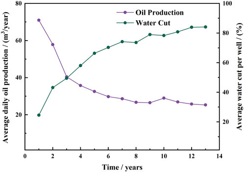
The Bohai Sea is in the northeast of China, and Q oilfield is located in the central Bohai Sea of China and is an offshore low-amplitude, bottom-water heavy oil reservoir with medium-to-high permeability. There are 40 sets of oil-water contacts in the Q oilfield. The oil and water layers alternate frequently. Different blocks, fault blocks, oil groups, oil layers, and sand bodies have different oil-water contacts. The reservoir is complex, and bottom water is widely distributed. As shown in Figure 1, the initial production of the Q oilfield was poor. The water-free production period was short, and the recovery rate was very low. The water cut increased quickly, and production declined rapidly. The bottom water coned into the wells very fast. After years of development with directional wells, the oilfield has now entered a ultra-high water cut stage. It is characterized by high water cut and low recovery rate. In the ultra-high water cut period, variations in water cut have a particularly significant impact on oil well production. Understanding the patterns of water cut changes during this phase is crucial for early detection and accurate prediction of abnormal conditions.

Figure 1

Figure 1. Annual average oil production and average water cut per well in the reservoir.

2.2 Data process

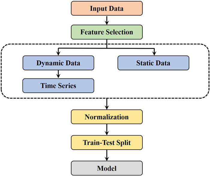
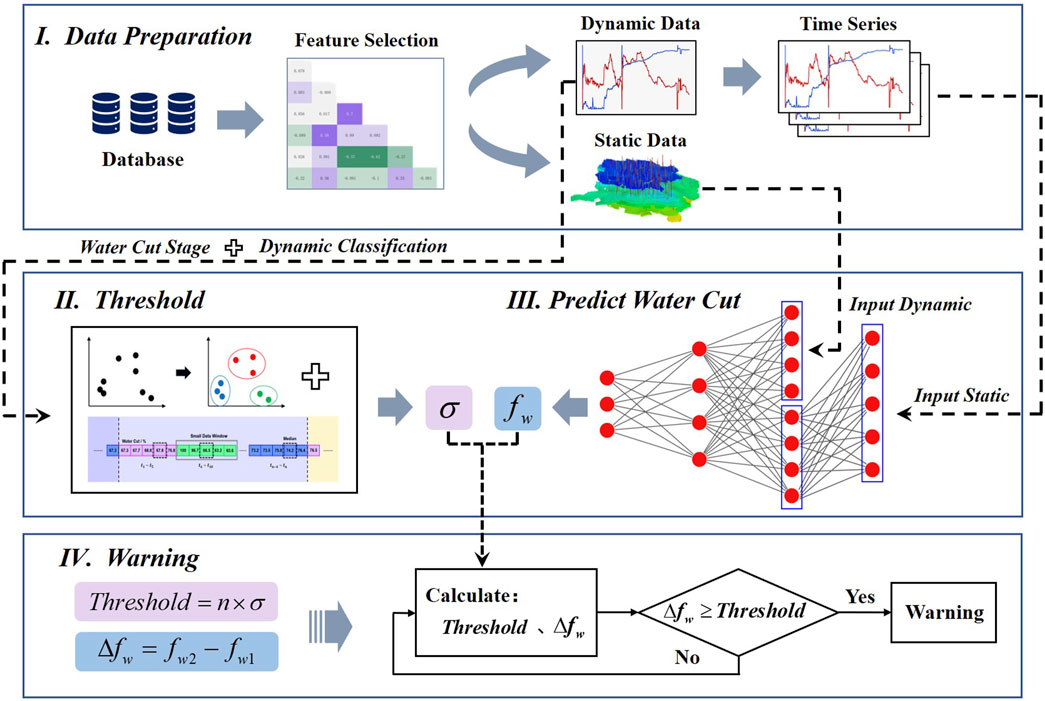
Figure 2 shows the data processing flowchart. First, the collected data undergoes feature selection to reduce the interference of redundant features on the model. Next, the selected dynamic features are transformed into a time-series format to fit the input requirements of the time-series model. Then, both dynamic and static features are normalized to eliminate the impact of magnitude differences on the model. Finally, the dataset is split into training and test sets in a 7:3 ratio and input into the model.

Figure 2

Figure 2. Data processing flowchart.

2.2.1 Dataset description

This study collected production data from 492 oil wells in the Q oilfield from 2001 to 2024, covering 22 features. The main features include oil pressure, casing pressure, back pressure, bottom hole flowing pressure, bottom hole temperature, pump inlet temperature, pump inlet pressure, pump outlet pressure, pump leakage current, pump current, pump motor temperature, pump voltage, pump frequency, pump vibration, wellhead temperature, choke size, gas-oil ratio, water cut, daily fluid production, daily gas production, daily water production, and daily oil production. Considering that well’s daily data log is partially missing and that daily data fluctuates greatly, the daily data is averaged on a monthly basis to obtain monthly averages, which are then used to construct the foundational dataset.

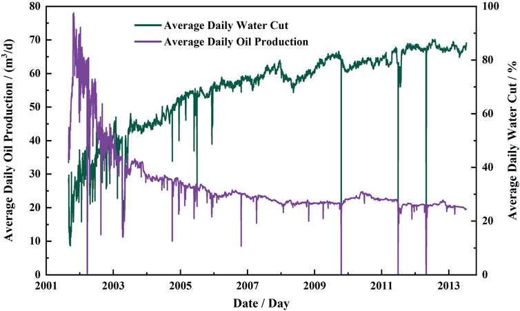
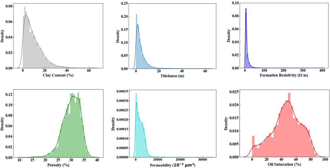
Figure 3 shows the average daily oil production and water cut for all wells from 2001 to 2013. Figure 4 is the logging data distribution of the reservoir sand body, including shale content, interlayer thickness, formation resistivity, porosity, permeability, and oil saturation.

Figure 3

Figure 3. Daily average oil production and water cut per Well.

Figure 4

Figure 4. Reservoir logging data statistics chart.

2.2.2 Feature selection

Dynamic data can reflect the production status and changing trends of oil wells in real-time. It is an important basis for predicting short-term well behavior, helping the model capture production trends and cyclic patterns. By effectively utilizing dynamic data, the water cut early warning system can more accurately predict the future production of oil wells, providing decision support and reducing potential economic losses. Static data describe the geological and engineering characteristics of the reservoir, offering fundamental information about the long-term production potential and behavior of the reservoir. Static data remain relatively stable throughout the life cycle of a well and are the basis for reservoir management and production optimization. By incorporating static data into the input of the LSTM model along with dynamic data, the model’s generalization ability and prediction accuracy can be improved.

Traditional time series prediction models often rely solely on time series data, neglecting the potential contributions of static features. The dataset constructed in this study comprehensively considers the influence of the reservoir, individual wells, and injector-producer well groups. It includes static parameters that reflect the geological characteristics of the wells as well as dynamic parameters that capture the production process. The rich feature dimensions provide machine learning models with sufficient information, helping to better capture the complex production patterns of oil wells.

Depending on the number of input features, data-driven prediction models can be divided into univariate and multivariate prediction methods. In this study, a multivariate prediction approach is adopted. Multivariate prediction considers multiple features simultaneously, providing the model with rich training samples and enhancing its generalization ability. However, too many features can increase the computational cost and risk of overfitting. Therefore, Pearson correlation coefficients are used in this study for feature selection.

The formula for Pearson correlation coefficient is as follows:

${\mathit{\rho }}_{\mathit{X},\mathit{Y}}=\frac{\mathit{c}\mathit{o}\mathit{v}\left(\mathit{X},\mathit{Y}\right)}{{\mathit{\sigma }}_{\mathit{X}}{\mathit{\sigma }}_{\mathit{Y}}}$

where $cov\left(X,Y\right)$ is the covariance between X and Y, $\text{with}{\sigma }_X$ and ${\sigma }_Y$ as their standard deviations.

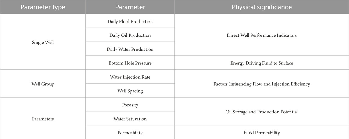
For each feature, the Pearson correlation coefficient with the water cut is calculated. The closer the absolute value of the Pearson correlation coefficient is to 1, the stronger the correlation between the two features. Six dynamic features were selected: daily fluid production, daily oil production, daily water production, bottom hole flowing pressure, injection volume (water injection from surrounding wells), and bottom hole flowing pressure. In addition, since water cut is also affected by static features, four static features were included: permeability, porosity, water saturation, and the distance between injector and producer wells.

The selected dynamic and static features comprehensively consider the impact of individual wells, well groups, and reservoirs, and each parameter has physical significance, as shown in Table 1.

Table 1

Table 1. Physical meaning of parameters.

2.2.3 Data normalization and splitting

Due to significant differences in the magnitude of the data, directly inputting the data into the model may negatively affect its performance. Normalization scales all features to the same range, reducing the differences in scale between different features, and thus improving the stability of the algorithm. The normalization formula is as follows:

${\mathit{X}}_{\mathit{n}\mathit{o}\mathit{r}\mathit{m}}=\frac{\mathit{X}-{\mathit{X}}_{\mathit{min}}}{{\mathit{X}}_{\mathit{max}}-{\mathit{X}}_{\mathit{min}}}$

where $X$ is the original feature, $X_{norm}$ is the normalized feature, $X_{\mathit{min}}$ is the minimum value of the feature, and $X_{\mathit{max}}$is the maximum value of the feature.

After normalization, the data are split into training and validation sets in a 7:3 ratio.

2.2.4 Time series transformation

By converting dynamic data into a sequence format, the dynamic data is restructured as the input format for the time series model. First, the time series data is segmented, grouping several consecutive time steps into one input sequence, with the corresponding future time steps selected as the model’s prediction target. Each input sequence contains the historical values of various production parameters, and these historical values retain their chronological order. By performing data shifting operations, past data is aligned and combined with data from subsequent time steps, allowing the model to capture production trends and dependencies from the historical data.

Next, the static features are integrated with the dynamic time series features through data concatenation. The static data is expanded to match the time dimension of the dynamic data, ensuring that each sample contains both dynamic features reflecting short-term changes and static features representing the long-term characteristics of the well.

3 Method and principle

After completing data processing, it is necessary to calculate the thresholds and predict the water cut values. If the change in water cut exceeds the threshold, an early warning is triggered; otherwise, the system remains in a safe state. The process of the early warning system is shown in Figure 5.

Figure 5

Figure 5. Early warning system flowchart.

3.1 Thresholds

3.1.1 Water cut stage division

During the production process of oil wells at different water cut stages, the impact of water cut changes on daily oil production varies significantly. For example, in wells at the ultra-high water cut stage, a 1% increase in water cut can have a significant negative impact on daily oil production, but a 1% increase in wells at the low water cut stage is generally within an acceptable range. Therefore, accurately dividing the water cut stages of oil wells is a critical part of the water cut early warning system. The criteria for different water cut stages are shown in Table 2.

Table 2

Table 2. Water cut stage division standards.

Due to the complex field conditions in the oilfield, operations such as well initiation, liquid discharge, and flowback can cause abnormal fluctuations in the water cut of oil wells. In extreme cases, the water cut may rise to 100%. These anomalies not only increase the noise in the water cut data but may also lead to misjudgment of the water cut stage, resulting in incorrect production decisions.

The sliding window method determines the water cut stage of the well by calculating the median within each small window and comprehensively analyzing the water cut data over a larger window that covers all well data. As shown in Figure 6, each small window contains 5 days of water cut data, while each large window contains n days of data (with n adjustable according to actual conditions). Compared to simple average calculations, the median is more robust in handling extreme and anomalous values, providing a more accurate reflection of the true water cut trend in the well. Additionally, using the median values from multiple consecutive small windows for comprehensive analysis effectively reduces misjudgments caused by short-term anomalies in a single window, ensuring the stability and reliability of stage division.

Figure 6

Figure 6. Water cut stage division method diagram.

3.1.2 Well classification

After completing the water cut stage division, further dynamic classification analysis of the wells is conducted. The classification is based on the average water cut and average daily oil production of each well at its current water cut stage. This classification considers the real-time dynamic performance of the wells during production, helping to reveal the impact of water cut changes on well production, and ensuring that more targeted and differentiated early warning strategies are applied to different types of wells.

The K-means clustering method is used for dynamic well classification. The main principle is to divide the objects in the dataset into $K$ clusters, minimizing the sum of the Euclidean distances from each object to the center of its cluster. Through iterative optimization, the clustering result ensures that objects within each cluster are as close as possible, while objects between different clusters are as far apart as possible. The main steps are as follows (Lloyd, 1982):

1. Randomly select $K$ data points as the initial cluster centers, and manually set the value of $K$.

2. Calculate the Euclidean distance between each data sample $x_i$ and the $K$ cluster centers, and assign each sample to the cluster with the nearest center. The formula for calculating Euclidean distance is as follows:

$\mathit{d}\left(\mathit{x},\mathit{y}\right)=\sqrt{{\displaystyle \sum _{\mathit{i}=\mathbf{1}}^{\mathit{n}}}{\left({\mathit{x}}_{\mathit{i}}-{\mathit{y}}_{\mathit{i}}\right)}^{\mathbf{2}}}$

where $x_i$ is the i-th data point, $y_i$ is the i-th cluster center, and $n$ is the dimension of the data.

3. For each cluster, recalculate the cluster center. The new cluster center is the mean of all data points in the cluster, and the formula is as follows:

${\mathit{y}}_{\mathit{i}}=\frac{\mathbf{1}}{\left|{\mathit{S}}_{\mathit{i}}\right|}{\displaystyle \sum _{\mathit{x}\in {\mathit{S}}_{\mathit{i}}}}\mathit{x}$

where $S_i$ is all the data points in cluster $i$.

4. Repeat steps 2 and 3 until the cluster centers no longer change significantly, at which point the clustering process is complete.

3.1.3 Threshold setting

Based on the previous water cut stage division and clustering results, the wells are classified into different categories. For each cluster, the change in water cut between consecutive time points is calculated and normalized to represent the change per unit time. By calculating the standard deviation ($\sigma$) of the water cut changes for each well cluster, the magnitude of water cut fluctuations during that stage is reflected. A larger $\sigma$ value indicates that the well’s production performance is more unstable during that stage.

The formula for calculating the early warning threshold is as follows:

$\mathit{T}\mathit{h}\mathit{r}\mathit{e}\mathit{s}\mathit{h}\mathit{o}\mathit{l}\mathit{d}=\mathit{n}\times \mathit{\sigma }$

where $n$ is the sensitivity coefficient set by field personnel, which can be adjusted flexibly according to different production requirements. It is recommended to set n between 1 and 3. Typically, n is set to 3. However, if greater sensitivity to changes is needed for early warnings, values of 2 or 1 can be used. Setting sensitivity too low may cause real issues to be overlooked, leading to underreporting, while setting it too high can result in unnecessary consumption of time and resources.

When the change in the water cut of a well exceeds the threshold $n\sigma$, the system triggers an early warning. This method fully considers the differences in sensitivity to water cut changes between wells, providing a scientifically based threshold grounded in statistical analysis. It not only captures abnormal situations but also effectively reduces false alarms and missed warnings, improving the precision and adaptability of the early warning system.

3.2 Model construction

3.2.1 LSTM principle

The Long Short-Term Memory (LSTM) model is an optimized version of the traditional Recurrent Neural Network (RNN) with strong memory capabilities, making it well-suited for handling time-series data. Its principles are as follows (Landi et al., 2021):

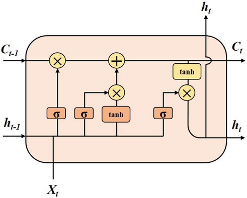
LSTM consists of a cell state, an input gate, an output gate, and a forget gate. The cell state can store values across arbitrary time intervals, and the three gates control how information enters and exits the cell. The forget gate compares the previous state with the current input and decides which information to retain or discard (1 means retain, 0 means forget). The input gate and the forget gate use the same mechanism to decide which information to update. The output gate determines which part of the cell state will be output, processes it, and produces the final output.

Figure 7 demonstrates the concatenation of internal cell states at different time steps. The four yellow rectangles in the figure represent the hidden layer structure of the network, with the symbols on top representing the activation functions used. The unit state concatenates the input $X_t$ at time $t$ and the output $h_{t-1}$ at time $t-1$, then performs forget or retain processing in the internal unit. In Figure 7, the horizontal line on the top controls long-term memory, while the one on the bottom controls short-term memory.

Figure 7

Figure 7. LSTM structure diagram.

This structure allows LSTM to effectively capture long-term dependencies in sequence data, making it highly suitable for time-series data processing.

In this study, a multi-input LSTM model was designed. The LSTM network, due to its ability to capture both long- and short-term dependencies in time-series data, is widely used in time-series prediction tasks. In this model, dynamic data is used as the time-series input, while static data is used as auxiliary input. This allows the model to capture the gradually changing dynamic information during well production, while also considering the fundamental geological characteristics of the well, thereby improving prediction accuracy.

The loss function used is Mean Squared Error (MSE), which measures the gap between the predicted values and the actual values. The Adam optimizer is employed to make the training process more stable and efficient, especially when handling large-scale data and complex model structures.

3.2.2 Network layer configuration

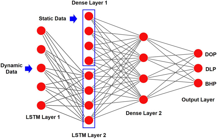
The model is composed of two LSTM layers and a fully connected layer, designed to achieve precise predictions for complex time series by integrating dynamic and static data. The model consists of two main components: one part processes dynamic data through the LSTM network to capture dependencies in the time series, while the other part processes static data through a fully connected layer, mapping it to the same feature space as the dynamic data. Finally, the features from these two parts are fused through concatenation, and the output layer generates predictions for Daily Oil Production (DOP), Daily Liquid Production (DLP), and Bottom Hole Pressure (BHP). The overall structure is shown in Figure 8.

Figure 8

Figure 8. Multi-input model network structure diagram.

First, the two LSTM layers in the model sequentially process the dynamic data. The first LSTM layer extracts short-term dependencies in the dynamic data and outputs an intermediate hidden state. The second LSTM layer further captures long-term dependencies in the time series, enhancing the model’s ability to understand and predict well production dynamics.

The input of the static data is processed through a fully connected layer. This fully connected layer applies a linear transformation and nonlinear activation function, mapping the static features to the same feature space as the LSTM hidden states. This process ensures that static features contribute effectively to the model’s predictions and eliminates potential conflicts when fusing dynamic and static features.

After processing through the two LSTM layers and the fully connected layer, the dynamic and static data features are concatenated in the feature space, forming a higher-dimensional feature representation. The concatenated feature vector is then passed through the fully connected output layer, where it undergoes a linear transformation to produce the final predictions.

3.3 Evaluation metrics

Based on whether the predicted values and actual values trigger an early warning, the results can be categorized into four types: True Positives (TP), False Positives (FP), True Negatives (TN), and False Negatives (FN). TP represents the number of samples where the early warning system correctly predicted an alert (both the predicted and actual values meet the early warning conditions). FP represents false alarms (the predicted value meets the early warning condition, but the actual value does not). TN represents correctly identified normal conditions (neither the predicted nor actual values meet the early warning conditions), and FN represents missed alarms (the predicted value does not meet the early warning condition, but the actual value does).

The effectiveness of the early warning system is measured using Accuracy, Precision, Recall, False Positive Rate (FPR), and False Negative Rate (FNR). The formulas are as follows:

$\mathit{A}\mathit{c}\mathit{c}\mathit{u}\mathit{r}\mathit{a}\mathit{c}\mathit{y}=\frac{\mathit{T}\mathit{P}+\mathit{T}\mathit{N}}{\mathit{T}\mathit{P}+\mathit{T}\mathit{N}+\mathit{F}\mathit{P}+\mathit{F}\mathit{N}}$

$\mathit{P}\mathit{r}\mathit{e}\mathit{c}\mathit{i}\mathit{s}\mathit{i}\mathit{o}\mathit{n}=\frac{\mathit{T}\mathit{P}}{\mathit{T}\mathit{P}+\mathit{F}\mathit{P}}$

$\mathit{R}\mathit{e}\mathit{c}\mathit{a}\mathit{l}\mathit{l}=\frac{\mathit{T}\mathit{P}}{\mathit{T}\mathit{P}+\mathit{F}\mathit{N}}$

$\mathit{F}\mathit{P}\mathit{R}=\frac{\mathit{F}\mathit{P}}{\mathit{F}\mathit{P}+\mathit{T}\mathit{N}}$

$\mathit{F}\mathit{N}\mathit{R}=\frac{\mathit{F}\mathit{N}}{\mathit{F}\mathit{N}+\mathit{T}\mathit{P}}$

Accuracy: Represents the proportion of samples where the system correctly predicts whether the well’s water cut is abnormal, without distinguishing between abnormal and normal conditions.

Precision: Represents the proportion of true anomalies among all the cases predicted as anomalies. A high precision indicates that the system effectively reduces false alarms.

Recall: Represents the proportion of correctly identified anomalies among all actual anomaly samples. A high recall rate indicates that the model can capture more anomaly cases.

FPR: Represents the proportion of normal samples that are incorrectly predicted as anomalies. A lower FPR means fewer false alarms.

FNR: Represents the proportion of actual anomaly samples that are not detected by the early warning system. A lower FNR means fewer missed alarms.

4 Results

4.1 Threshold calculation

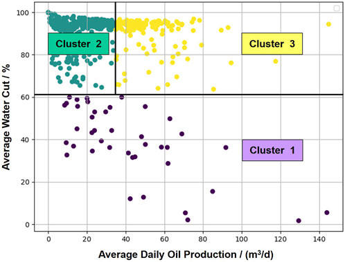
First, the sliding window method is used to determine the current water cut stage of the well. Then, based on the current water cut stage and daily oil production of each well, the wells are classified into three categories using the K-means algorithm. The classification results are shown in Figure 9, where Cluster 1 represents low water cut wells (42 wells), Cluster 2 represents high water cut wells with weak production capacity (304 wells), and Cluster 3 represents high water cut wells with strong production capacity (145 wells).

Figure 9

Figure 9. Dynamic well classification results.

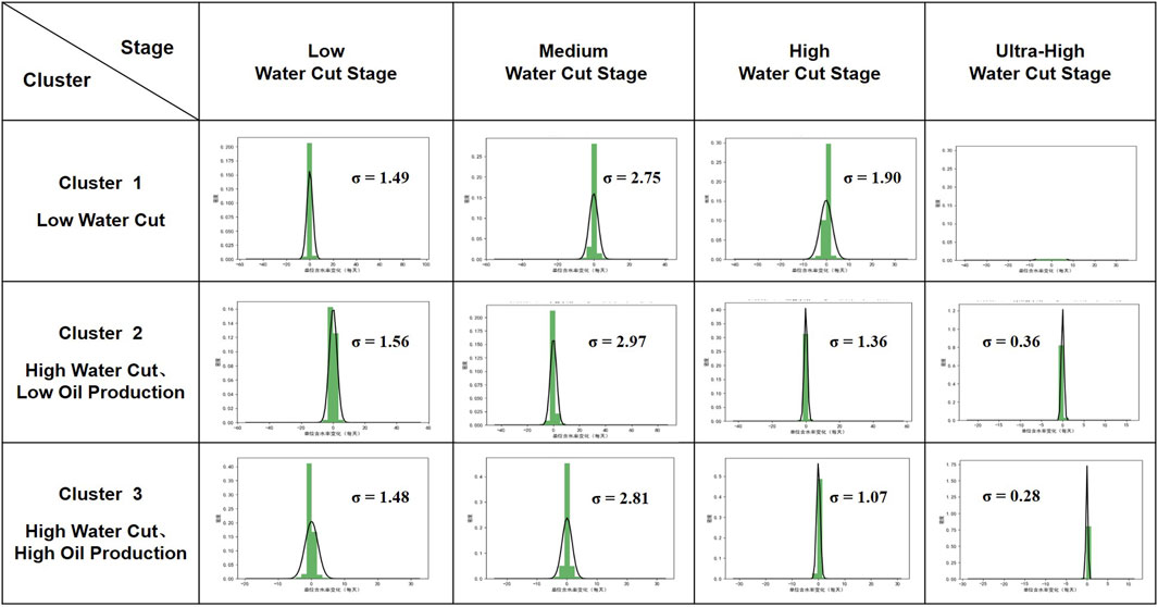
Based on the dynamic classification results and the current water cut stage of each well, the data is grouped, and the difference in water cut between consecutive time points is calculated to obtain the change in water cut per unit time. Statistical analysis is then performed on these difference values to obtain the standard deviation $\sigma$, as shown in Figure 10. Notably, there is no ultra-high water cut stage for wells in Cluster 1.

Figure 10

Figure 10. Standard deviation for different water cut stages and well clusters.

From the perspective of water cut stages, the medium water cut stage has the highest $\sigma$ value, indicating that water invasion intensifies during this stage, leading to greater fluctuations in the water cut. The ultra-high water cut stage has the lowest $\sigma$ value, reflecting that the well has entered a stable water flooding stage, where the reservoir is primarily water-driven and the water cut fluctuates less.

From the perspective of well categories, Cluster 3 wells have lower $\sigma$ values at all stages. Upon investigation, it was found that these wells have implemented effective water flooding management and pressure maintenance measures, which have controlled the fluctuations in water cut during production.

4.2 Optimal time step selection

Before optimizing the time step, it is necessary to determine the time interval. Given that the daily water cut in field data fluctuates frequently and lacks clear patterns, the average daily water cut for each month is used as the early warning indicator. Using monthly averages significantly reduces abnormal fluctuations in the data. The LSTM model is then employed to capture long-term trends, resulting in higher accuracy and reliability. As a result, the model’s time interval is set to 1 month, making it easier to process the monthly average data.

The input and output time steps have a significant impact on the prediction results of the model. If the time step is too short, it may not provide enough information for the model, while a time step that is too long may introduce irrelevant information, leading to overfitting. Therefore, this early warning system optimizes the best time step combinations for different data samples to ensure the stability and accuracy of the model’s predictions. The evaluation metric used is the Mean Absolute Percentage Error (MAPE). By standardizing the error, MAPE provides an objective reflection of the model’s performance across different time steps. The calculation formula is as follows:

$\mathit{M}\mathit{A}\mathit{P}\mathit{E}=\frac{\mathbf{1}}{\mathit{n}}{\displaystyle \sum _{\mathit{i}=\mathbf{1}}^{\mathit{n}}}\left|\frac{{\mathit{y}}_{\mathit{i}}-{\widehat{\mathit{y}}}_{\mathit{i}}}{{\mathit{y}}_{\mathit{i}}}\right|\times \mathbf{100}\%$

where $y_i$ is the actual water cut value, ${\widehat{y}}_i$ is the predicted water cut value, and $n$ is the number of data points.

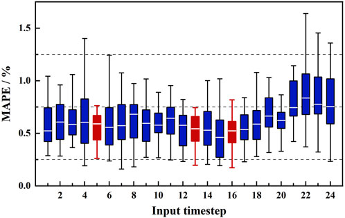
Figure 11 shows the water cut prediction errors under different input time steps (with outliers removed). Each box represents the errors for output time steps ranging from 1 to 24 at a given input step. When the box is relatively low and the whiskers are short, it indicates that the errors are smaller and less volatile, suggesting higher accuracy and stability. Three red boxes (steps 5, 13, and 16) show relatively short heights and whisker lengths, with lower and more stable errors, warranting further analysis.

Figure 11

Figure 11. Relationship between input time steps and prediction error.

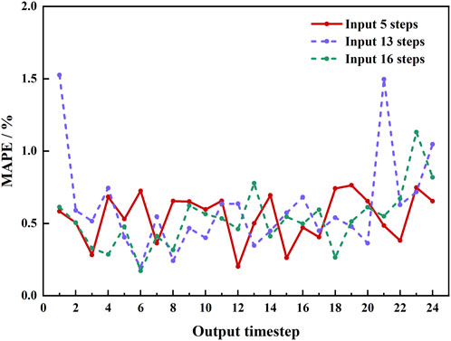
Figure 12 illustrates the water cut errors at different output time steps, with three lines representing the prediction errors for input steps of 5, 13, and 16. It can be seen that when the input time step is 5, the model’s overall errors remain at a low level without significant error peaks, indicating that an input time step of 5 is more suitable for predicting water cut. Additionally, when the output time step is 12, the model error reaches its lowest point. Therefore, the final selected time step combination is: input time step of 5 and output time step of 12.

Figure 12

Figure 12. Relationship between output time steps and prediction error.

4.3 Early warning results

The calculated thresholds (set at 1 times $\sigma$) and the established model were used to perform water cut early warnings for the wells.

Figure 13 shows the early warning results for predicted water cut, comparing the dual-driven model trained with both dynamic and static data, and the single-driven model trained with only dynamic data.

Figure 13

Figure 13. Water cut warning results for different models. (A) Model trained with dynamic and static features; (B) Model trained with dynamic features only.

The five evaluation metrics were calculated based on the early warning results, and the results are shown in Table 3. By analyzing these metrics, a comprehensive assessment of the system’s early warning performance for abnormal situations can be made, providing quantitative insights for optimizing the early warning system.

Table 3

Table 3. Performance metrics of the early warning system.

As shown in Figure 14, this figure presents a comparison of several key performance metrics between the model considering both dynamic and static features (dual-driven model) and the model considering only dynamic features (single-driven model) in the early warning of water cut in oil wells. It is evident that the dual-driven model outperforms the single-driven model across all metrics.

Figure 14

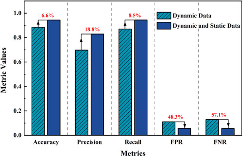
Figure 14. Comparison of early warning metrics between dynamic features only and dynamic-static features.

Specifically, compared to the single-driven model, the dual-driven model improved Accuracy, Precision, and Recall by 6.6%, 18.8%, and 8.5%, respectively. Additionally, the FPR and FNR were reduced by 48.3% and 57.1%, respectively. This indicates that the dual-driven model not only performs better in terms of overall early warning accuracy but also improves the ability to reduce false alarms and missed alarms, effectively enhancing the validity and reliability of the early warning system.

5 Discussions

This paper establishes an oil well production early warning method based on water cut variation, achieving an accuracy of 94.34% in predicting abnormal water cut changes in oil well production. The proposed method can guide the field in adjusting injection and production parameters in advance to prevent water cut increases and can also be used for optimizing injection and production parameters. Compared with related cases, the innovation and limitations of the proposed method are mainly reflected in the following two aspects:

(1) Comparison with Existing Water Cut Prediction Methods and Early Warning Methods:

Conventional water cut prediction methods have many limitations. In recent years, machine learning methods have gained popularity, primarily applied to the prediction of production dynamics. A few scholars have also conducted research on water cut prediction. For example, Ahmadi et al. (2019) employed a data-driven approach to classify saline oil wells and used an autoregressive (AR) model to create the regression relationship between salinity and water cut. This method established the relationship between salinity and water cut, but its application is highly limited in other types of reservoirs, as it only considers the relationship between salinity and water cut, overlooking other potential factors. Abdalla et al. (2023) developed a data-driven modeling approach based on actual electric submersible pump datasets. This method analyzes and processes real field data using various machine learning algorithms to predict flow rates and water cut. The method is applicable for filling in measurement data and predicting the water cut for the current day, but it is not suitable for predicting future water cut levels. Furthermore, this approach only considers dynamic parameters such as pump pressure and bottomhole flowing pressure, with insufficient consideration of static parameters.

The method proposed in this study differs from the two methods mentioned above. This method employs a data-driven model architecture that combines dynamic and static parameters, enabling the simultaneous consideration of oil well dynamics and geological parameters for water cut prediction. Compared to Ahmadi et al.’s approach, it is more comprehensive, and its focus is different from that of Ahmadi et al., who establish a relationship between salinity and water cut. Ramez’s method considers dynamic parameters like pump pressure and bottomhole flowing pressure, but it does not account for static geological parameters. Moreover, Ramez’s method is only applicable when dynamic conditions are known, primarily for predicting the current day’s water cut, and it cannot forecast future water cut changes. The method proposed in this paper, by considering both dynamic well parameters and static geological parameters, achieves the prediction of future water cut levels. While the water cut prediction method in this paper is similar to the production rate prediction methods proposed by Werneck, Kumar, and others (Werneck et al., 2022; Kumar et al., 2023), the key difference is that this study does not incorporate the attention mechanism but introduces static geological parameters. The introduction of static geological data makes this method more suitable for the early warning of water cut rise in highly heterogeneous reservoirs.

In terms of early warning methods, many studies have established the relationship between predictive parameters and warning results, with related research primarily focusing on oil well operating conditions, while some studies focus on well dynamic parameters research. For example, the operational risk prediction model proposed by Mamudu et al. (2022) can effectively assess the dynamic risks of oil wells. The method in this paper is similar to the approach proposed by Zhong et al. (2016), where prediction precedes warning. The difference is that this study determines the thresholds for oil wells in a more reasonable manner by classifying them and setting phased thresholds. And the method proposed by Zhong is a probabilistic prediction model. Compared with this early warning model, the method proposed in this paper provides a more direct early warning, and the early warning result is more clear.

(2) Applicability to Specific Reservoir Conditions:

Most of the early warning methods are set according to the operating conditions of specific reservoirs, and there are few studies on well dynamic parameter early warning (Bayazitova et al., 2024; Harrouz et al., 2024; Gatta et al., 2024; Mamudu et al., 2022; Zhong et al., 2016). The prediction before warning method adopted in this study is a kind of dynamic parameter early warning method. The establishment of prediction model determines the applicability of this method. And it is found that most of the water cut prediction methods have many limitations, some of them are limited in the applicability of the reservoir, and some of them are not comprehensive (Ahmadi et al., 2019; Abdalla et al., 2023). The method in this study takes into account the influence of static geological parameters, and the permeability, porosity, sand body thickness and other parameters can improve the prediction ability of the model in the high water cut period. Therefore, the proposed method is suitable for medium-to-high permeability reservoirs under long-term water drive. However, to apply it to ultra-low permeability reservoirs with long-term water drive, it would be necessary to incorporate considerations of fractures. Therefore, it is worth exploring to add fracture parameters such as fracture intensity, length and width to appropriate network layers and combine them with other parameters to improve the model and make it suitable for reservoirs with fractures.

6 Conclusion

This study aims to establish a more accurate early warning system for oil well production in medium-to-high-permeability reservoirs under long-term water flooding. The research conclusions are as follows:

(1) The method proposed in this study considers both dynamic and static characteristics of oil wells, effectively improving the accuracy of early warnings. Compared to models that only consider dynamic features, the proposed approach increases early warning accuracy by 6.6%.

(2) The proposed method classifies oil wells and incorporates stage-specific early warning thresholds, significantly enhancing its adaptability to different well conditions and reducing false and missed alarms.

(3) The research method in this study is very effective in medium and high permeability reservoirs with long-term water drive, and its application in other reservoirs remains to be explored.

(4) The early warning system can predict abnormal increases in water cut in advance, enabling improvements in well group injection and production strategies to prevent surges in water cut. Additionally, it can be used for optimizing injection and production parameters of oil wells.

Data availability statement

The data analyzed in this study is subject to the following licenses/restrictions: The data sets presented in this article are not readily available as they were obtained from CNOOC Tianjin Branch and are subject to the company’s confidentiality policy. Data sets are available from corresponding author with permission from CNOOC Tianjin Branch. Requests to access these datasets should be directed to cWluZ3NodWFuZy5KaW5AMTYzLmNvbQ==.

Author contributions

JL: Conceptualization, Funding acquisition, Methodology, Project administration, Resources, Validation, Writing–original draft, Writing–review and editing. CZ: Conceptualization, Methodology, Supervision, Visualization, Writing–review and editing. YaL: Software, Validation, Writing–review and editing. YiL: Formal Analysis, Validation, Writing–review and editing. QJ: Investigation, Writing–review and editing. TX: Data curation, Writing–review and editing. XL: Writing–original draft. YZ: Investigation, Writing–review and editing.

Funding

The author(s) declare that financial support was received for the research, authorship, and/or publication of this article. This research was funded by “14th Five-Year Plan” Major Science and Technology Projects of China National Offshore Oil Corporation, grant number KJGG-2022-15-0303, and the APC was funded by China National Offshore Oil Corporation.

Conflict of interest

Authors JL, CZ, YaL, YiL and TX CNOOC (China) Limited Tianjin branch.

The remaining authors declare that the research was conducted in the absence of any commercial or financial relationships that could be construed as a potential conflict of interest.

The authors declare that this study received funding from China National Offshore Oil Corporation. The funder was not involved in the study design, collection, analysis, interpretation of data, or the writing of this article, but the decision to submit it for publication was approved by the funder.

Generative AI statement

The author(s) declare that Generative AI was used in the creation of this manuscript. We improved the article language with generative AI.

Publisher’s note

All claims expressed in this article are solely those of the authors and do not necessarily represent those of their affiliated organizations, or those of the publisher, the editors and the reviewers. Any product that may be evaluated in this article, or claim that may be made by its manufacturer, is not guaranteed or endorsed by the publisher.

References

Abdalla, R., Al-Hakimi, W., Perozo, N., and Jaeger, P. (2023). Real-time liquid rate and water cut prediction from the electrical submersible pump sensors data using machine-learning algorithms. ACS Omega 8 (14), 12671–12692. doi:10.1021/acsomega.2c07609

PubMed Abstract | CrossRef Full Text | Google Scholar

Abramov, V. O., Abramova, A. V., Bayazitov, V. M., Marnosov, A. V., Kuleshov, S. P., and Gerasin, A. S. (2016). Selective ultrasonic treatment of perforation zones in horizontal oil wells for water cut reduction. Appl. Acoust. 103, 214–220. doi:10.1016/j.apacoust.2015.06.017

CrossRef Full Text | Google Scholar

Ahmadi, R., Shahrabi, J., and Aminshahidy, B. (2019). Water cut/salt content forecasting in oil wells using a novel data-driven approach. Oil and Gas Sci. Technol. 74, 68. doi:10.2516/ogst/2019040

CrossRef Full Text | Google Scholar

Ahn, S., Lee, K., Choe, J., and Jeong, D. (2023). Numerical approach on production optimization of high water-cut well via advanced completion management using flow control valves. J. Petroleum Explor. Prod. Technol. 13 (7), 1611–1625. doi:10.1007/s13202-023-01632-3

CrossRef Full Text | Google Scholar

Alfarge, D., Wei, M., Bai, B., and Almansour, A. (2018). Numerical simulation study to understand the performance of rpm gels in water-shutoff treatments. J. Petroleum Sci. Eng. 171, S092041051830665X. doi:10.1016/j.petrol.2018.07.082

CrossRef Full Text | Google Scholar

Bahaloo, S., Mehrizadeh, M., and Najafi-Marghmaleki, A. (2023). Review of application of artificial intelligence techniques in petroleum operations. Pet. Res. 8 (2), 167–182. doi:10.1016/j.ptlrs.2022.07.002

CrossRef Full Text | Google Scholar

Batista, F. A., Coutinho, B. G., Marcondes, F., de Farias Neto, S. R., and de Lima, A. G. B. (2011). Two-phase flow of an oil-water system in porous media with complex geometry including water flooding: modeling and simulation. J. Porous Media 14 (7), 579–592. doi:10.1615/jpormedia.v14.i7.20

CrossRef Full Text | Google Scholar

Bayazitova, G., Anastasiadou, M., and dos Santos, V. D. (2024). Oil and gas flow anomaly detection on offshore naturally flowing wells using deep neural networks. Geoenergy Sci. Eng. 242, 213240. doi:10.1016/j.geoen.2024.213240

CrossRef Full Text | Google Scholar

Clarkson, C. R. (2013). Production data analysis of unconventional gas wells: review of theory and best practices. Int. J. Coal Geol. 109–110, 101–146. doi:10.1016/j.coal.2013.01.002

PubMed Abstract | CrossRef Full Text | Google Scholar

Dhaif, R. A., Ibrahim, A. F., Elkatatny, S., and Shehri, D. A. (2021). Prediction of oil rates using machine learning for high gas oil ratio and water cut reservoirs. Flow Meas. Instrum. 82, 102065. doi:10.1016/j.flowmeasinst.2021.102065

CrossRef Full Text | Google Scholar

Elmabrouk, S., Shirif, E., and Mayorga, R. J. P. S. (2014). Artificial neural network modeling for the prediction of oil production. Petroleum Sci. Technol. 32 (9), 1123–1130. doi:10.1080/10916466.2011.605093

CrossRef Full Text | Google Scholar

Gatta, F., Giampaolo, F., Chiaro, D., and Piccialli, F. (2024). Predictive maintenance for offshore oil wells by means of deep learning features extraction. Expert Syst. 41 (2), e13128. doi:10.1111/exsy.13128

CrossRef Full Text | Google Scholar

Grishchenko, V. A., Pozhitkova, S. S., Mukhametshin, V.Sh., and Yakupov, R. F. (2021). Water cut forecast after downhole pumping equipment optimization based on displacement characteristics. SOCAR Proc. SI2, 143–151. doi:10.5510/OGP2021SI200582

CrossRef Full Text | Google Scholar

Harrouz, A., Salem, H., Toubakh, H., Kafi, R. M., and Sayed-Mouchaweh, M. (2024). Fault prognosis of subsurface safety valve system with limited real data using self-adaptive neural network. Evol. Syst. 15 (3), 899–917. doi:10.1007/s12530-023-09525-w

CrossRef Full Text | Google Scholar

Hunyinbo, S., Azom, P., Ben-Zvi, A., and Y. Leung, J. (2023). A machine learning approach to real-time uncertainty assessment of SAGD forecasts. SPE J. 28 (1), 342–354. doi:10.2118/208962-PA

CrossRef Full Text | Google Scholar

Ibrahim, N. M., Alharbi, A. A., Alzahrani, T. A., Abdulkarim, A. M., Alessa, I. A., Hameed, A. M., et al. (2022). Well performance classification and prediction: deep learning and machine learning long term regression experiments on oil, gas, and water production. Sensors 22 (14), 5326. doi:10.3390/s22145326

PubMed Abstract | CrossRef Full Text | Google Scholar

Kaleem, W., Tewari, S., Fogat, M., and Martyushev, D. A. (2024). A hybrid machine learning approach based study of production forecasting and factors influencing the multiphase flow through surface chokes. Petroleum 10 (2), 354–371. doi:10.1016/j.petlm.2023.06.001

CrossRef Full Text | Google Scholar

Kamari, A., Mohammadi, A. H., and Ramjugernath, D. (2018). Data-driven modeling for determination of asphaltene stability condition in oil system. Petroleum Sci. Technol. 36 (11), 726–731. doi:10.1080/10916466.2018.1445100

CrossRef Full Text | Google Scholar

Khamehchi, E., and Bemani, A. (2020). Prediction of pressure in different two-phase flow conditions: machine learning applications. Measurement 173, 108665. doi:10.1016/j.measurement.2020.108665

CrossRef Full Text | Google Scholar

Kumar, I., Tripathi, B. K., and Singh, A. (2023). Attention-based LSTM network-assisted time series forecasting models for petroleum production. Eng. Appl. Artif. Intell. 123, 106440. doi:10.1016/j.engappai.2023.106440

CrossRef Full Text | Google Scholar

Landi, F., Baraldi, L., Cornia, M., and Cucchiara, R. (2021). Working memory connections for LSTM. Neural Netw. 144, 334–341. doi:10.1016/j.neunet.2021.08.030

PubMed Abstract | CrossRef Full Text | Google Scholar

Lloyd, S. (1982). Least squares quantization in PCM. IEEE Trans. Inf. Theory 28 (2), 129–137. doi:10.1109/tit.1982.1056489

CrossRef Full Text | Google Scholar

Ma, X., and Liu, Z. (2018). Predicting the oil production using the novel multivariate nonlinear model based on arps decline model and kernel method. Neural Comput. and Applic 29 (2), 579–591. doi:10.1007/s00521-016-2721-x

CrossRef Full Text | Google Scholar

Mamudu, A., Khan, F., Zendehboudi, S., and Adedigba, S. (2022). Logic-based data-driven operational risk model for augmented downhole petroleum production systems. Comput. and Chem. Eng. 165, 107914. doi:10.1016/j.compchemeng.2022.107914

CrossRef Full Text | Google Scholar

Meshalkin, V. P., Yakubov, R. N., Lenchenkova, L. E., and Chelnokov, V. V. (2021). Computer modeling of the integrated chemical engineering process of water shutoff of high-water-cut oil-bearing porous rock formations. Dokl. Chem. 501 (1), 243–247. doi:10.1134/s0012500821110045

CrossRef Full Text | Google Scholar

Miah, M. I., Ahmed, S., Zendehboudi, S., and Butt, S. (2020). Machine learning approach to model rock strength: prediction and variable selection with aid of log data. Rock Mech. Rock Eng. 53, 4691–4715. doi:10.1007/s00603-020-02184-2

CrossRef Full Text | Google Scholar

Nagao, M., Datta-Gupta, A., Onishi, T., and Sankaran, S. (2024). Physics informed machine learning for reservoir connectivity identification and robust production forecasting. SPE J. 29 (9), 4527–4541. doi:10.2118/219773-PA

CrossRef Full Text | Google Scholar

Nikitin, N. O., Revin, I., Hvatov, A., Vychuzhanin, P., and Kalyuzhnaya, A. V. . (2021). Hybrid and automated machine learning approaches for oil fields development: the case study of volve field.

Google Scholar

Onalo, D., Adedigba, S., Oloruntobi, O., Khan, F., James, L. A., and Butt, S. (2020). Data-driven model for shear wave transit time prediction for formation evaluation. J. Petroleum Explor. Prod. Technol. 10, 1429–1447. doi:10.1007/s13202-020-00843-2

CrossRef Full Text | Google Scholar

Pinilla, A., Asuaje, M., Pantoja, C., Ramirez, L., Gomez, J., and Ratkovich, N. (2021). CFD study of the water production in mature heavy oil fields with horizontal wells. PLOS One 16 (10), e0258870. doi:10.1371/journal.pone.0258870

PubMed Abstract | CrossRef Full Text | Google Scholar

Pratikto, F., Indratno, S., Suryadi, K., and Santoso, D. (2023). A data-driven approach to estimating post-discovery parameters of unexplored oilfields. Petroleum 9 (2), 285–300. doi:10.1016/j.petlm.2022.10.001

CrossRef Full Text | Google Scholar

Sadeqi-Arani, Z., and Kadkhodaie, A. (2023). A bibliometric analysis of the application of machine learning methods in the petroleum industry. Results Eng. 20, 101518. doi:10.1016/j.rineng.2023.101518

CrossRef Full Text | Google Scholar

Shabdirova, A., Minh, N. H., and Zhao, Y. (2019). A sand production prediction model for weak sandstone reservoir in Kazakhstan. J. Rock Mech. Geotechnical Eng. 11 (4), 760–769. doi:10.1016/j.jrmge.2018.12.015

CrossRef Full Text | Google Scholar

Shah, M. S., Khan, F., Zendehboudi, S., and Abbas, M. (2023). A hybrid connectionist enhanced oil recovery model with real-time probabilistic risk assessment. Geoenergy Sci. Eng. 227, 211760. doi:10.1016/j.geoen.2023.211760

CrossRef Full Text | Google Scholar

Sircar, A., Yadav, K., Rayavarapu, K., Bist, N., and Oza, H. (2021). Application of machine learning and artificial intelligence in oil and gas industry. Petroleum Res. 6 (4), 379–391. doi:10.1016/j.ptlrs.2021.05.009

CrossRef Full Text | Google Scholar

Tadjer, A., Hong, A., and Bratvold, R. B. (2021). Machine learning based decline curve analysis for short-term oil production forecast. Energy Explor. and Exploitation 39 (5), 1747–1769. doi:10.1177/01445987211011784

CrossRef Full Text | Google Scholar

Wang, H., Mu, L., Shi, F., and Dou, H. (2020). Production prediction at ultra-high water cut stage via recurrent neural network. Petroleum Explor. Dev. 47 (5), 1084–1090. doi:10.1016/S1876-3804(20)60119-7

CrossRef Full Text | Google Scholar

Wang, J., Shi, C., Ji, S., Li, G., and Chen, Y. (2017). New water drive characteristic curves at ultra-high water cut stage. Petroleum Explor. Dev. 44 (6), 1010–1015. doi:10.1016/S1876-3804(17)30113-1

CrossRef Full Text | Google Scholar

Werneck, R. de O., Prates, R., Moura, R., Gonçalves, M. M., Castro, M., Soriano-Vargas, A., et al. (2022). Data-driven deep-learning forecasting for oil production and pressure. J. Pet. Sci. Eng. 210, 109937. doi:10.1016/j.petrol.2021.109937

CrossRef Full Text | Google Scholar

Wu, Y., Mi, L., Ma, L., Zheng, R., and Feng, X. (2024a). Rate transient analysis for multi-fractured wells in tight gas reservoirs considering multiple nonlinear flow mechanisms. Water 16 (13), 1866. doi:10.3390/w16131866

CrossRef Full Text | Google Scholar

Wu, Y., Mi, L., Zheng, R., Ma, L., and Feng, X. (2024c). A practical semi-analytical model for production prediction of fractured tight gas wells with multiple nonlinear flow mechanisms. Arab. J. Sci. Eng. doi:10.1007/s13369-024-09176-2

CrossRef Full Text | Google Scholar

Wu, Y., Zheng, R., Ma, L., and Feng, X. (2024b). Uncertainty quantification in rate transient analysis of multi-fractured tight gas wells exhibiting gas–water two-phase flow. Water 16 (19), 2744. doi:10.3390/w16192744

CrossRef Full Text | Google Scholar

Zhong, Y., Liu, Y., Lin, X., and Luo, S. (2016). The method of oilfield development risk forecasting and early warning using revised bayesian network. Math. Problems Eng. 2016 (1), 9564801–9564810. doi:10.1155/2016/9564801

CrossRef Full Text | Google Scholar