 Weihao Zhang
94% of researchers rate our articles as excellent or good
Learn more about the work of our research integrity team to safeguard the quality of each article we publish.
Find out more
ORIGINAL RESEARCH article
Front. Earth Sci., 09 April 2024
Sec. Geochemistry
Volume 12 - 2024 | https://doi.org/10.3389/feart.2024.1394094
This article is part of the Research TopicUnconventional Resources: Provenance Analysis, Sediment Transport, Reservoir Evaluation, Geo-energyView all 29 articles
The borehole-ground transient electromagnetic method enhances the detection range and resolution by placing the transmitter electrode within the borehole, allowing for close-proximity excitation of subsurface targets and compensating for the shortcomings of traditional ground-based methods. Utilizing an unstructured vector finite element method combined with a second-order backward Euler variable time-stepping difference scheme and the MUMPS solver, we have achieved three-dimensional forward modeling simulation of the transient electromagnetic field for a borehole-ground electric source. Based on the validation of its accuracy, we analyzed the effectiveness of this method for dynamic monitoring of shale gas reservoir fracturing. Through forward modeling, we examined the characteristics of the radial electric field response during shale gas reservoir fracturing monitoring and evaluated the effectiveness of the borehole-ground TEM method in dynamic monitoring of shale gas reservoirs. The research results indicate that this method can meet the requirements for reservoir fracturing dynamic monitoring and has a promising application prospect.
In recent years, as unconventional oil and gas utilization enter a late stage of development into areas where the water cut is high, research on the identification of oil, gas, and water; the prediction of the residual oil and gas distribution; and the dynamic monitoring of oil reservoirs has become crucial (Hu et al., 2014; Zhao et al., 2019). Hydraulic fracturing is a key technology in the development of unconventional oil and gas reservoirs that directly affects the production of unconventional oil and gas. The forward simulation of hydraulic fracturing dynamic monitoring models can not only verify the effectiveness of hydraulic fracturing, but also provides important guidance for the hydraulic fracturing of unconventional oil and gas. Although techniques such as the time-lapse seismic method have matured, during hydraulic fracturing, the small difference in the acoustic impedance caused by the displacement of reservoir fluids by fracturing fluids makes data interpretation difficult, and this method is also costly. Therefore, geophysical methods such as time-lapse gravity and time-lapse electromagnetic models are beginning to be developed (Peng et al., 2012). Notably, the displacement of fracturing fluids can cause significant changes in reservoir electrical properties, providing a theoretical basis for the application of electromagnetic exploration techniques in the dynamic monitoring of unconventional oil and gas reservoirs.
With the increasing demand for the exploration of deep-seated resources, several limitations in conventional ground-based electromagnetic surveying techniques for deep resource exploration have been identified. To address these issues, two approaches can be pursued. First, increasing the transmit power of the excitation field source to improve the signal-to-noise ratio of the received electromagnetic signals can enhance the practicality and effectiveness of electromagnetic methods. Second, facilities such as tunnels, mines, and boreholes can be used to place a transmitter under-ground and close to the target body for emission stimulation. This not only allows for the acquisition of stronger abnormal response signals, thereby increasing the detection depth, but also enhances the resolution of the abnormal body.
The transient electromagnetic method has been widely applied in environmental surveys, oil and gas exploration, mineral exploration, geothermal resource exploration, and deep crustal studies. Compared to controlled-source electromagnetic (CSEM) and magnetotelluric (MT) methods, this method has several advantages, such as a greater detection depth and a higher signal-to-noise ratio (Keller et al., 1984; Strack, 1984; Hördt et al., 1992; Mitsuhata et al., 2002; Müller et al., 2002; Commer et al., 2006; Haroon et al., 2015; He and Xue, 2018). The rational interpretation of electromagnetic data relies on forward and inversion techniques, and forward simulation plays a crucial role by providing important guidance for oil and gas reservoir development. Therefore, this topic has been the focus of widespread attention by scholars.
Current research on time-domain electromagnetic methods primarily focuses on numerical simulation and feasibility analysis. In the field of borehole transient electromagnetic technology, the borehole electrical method was initially proposed by researchers in the former Soviet Union for the delineation of coal seam horizons. He Zhanxiang further developed the borehole time-frequency electromagnetic method based on previous research, deriving a three-dimensional numerical simulation algorithm for vertical dipole sources using the volume integral equation method, and achieved three-dimensional forward and inversion modeling of borehole electromagnetic methods (Wang et al., 2006; Wang et al., 2007). Ke Ganpan and Huang Qinghua used finite element methods to implement three-dimensional forward simulation of vertical line source electric fields (Ke and Huang, 2009). Cuevas established a borehole electromagnetic model that involved placing vertical electric dipole sources as excitation sources at the bottom of the metal casing. In addition, Cuevas analyzed the electromagnetic response characteristics at the radial distance measurement points on the ground and studied the effects of factors such as the length and conductivity of the metal casing on the response (Cuevas, 2012). Ghada and Sami conducted time-domain numerical simulations of infinitely long wire sources in two-layered formations and analyzed the influences of different layer conductivities on the response results (Ghada and Al-Najim, 2015). Zhang Jiaqi integrated the expressions for each component of the dipole electromagnetic field along the direction of the wire to obtain analytical expressions for the vertical long wire source’s electromagnetic field, and compared the responses of this field with the response of the ground horizontal electric dipole as part of a three-dimensional forward simulation of a borehole. This demonstrated the significant advantages of borehole electromagnetic methods in deep resource detection compared to conventional ground-based methods (Zhang, 2018). In terms of dynamic monitoring, Orange et al. analyzed the feasibility of using marine controlled-source electromagnetic methods to monitor the process of oil and gas reservoir development based on a classic two-dimensional oil and gas model (Orange et al., 2009). Furthermore, Wirianto et al. studied the feasibility of using land-based controlled-source electromagnetic methods to monitor changes in oil and gas reservoirs through numerical simulations of complex three-dimensional resistivity models (Wirianto et al., 2010). Meanwhile, Xie Xingbing et al. conducted experiments on residual oil monitoring using time-domain long-offset transient electromagnetic methods and preliminarily verified the effectiveness of this method in detecting residual oil boundaries (Xie et al., 2016). Li et al. proposed a multi-source, multi-directional ground-to-well vertical electromagnetic profiling method and used the integral equation method to simulate the electromagnetic response characteristics of oil and gas reservoir resistivity and oil saturation changes during water injection and production processes (Li et al., 2017). Liu et al. conducted numerical simulations and field experiments on the hydraulic fracturing process of shale gas fields and confirmed the good effect of controlled-source electromagnetic methods in monitoring shale gas production (Liu R. et al., 2020). Wang Xinyu et al. conducted a simulation and performed an analysis of the dynamic monitoring of oil reservoirs using electrical source transient electromagnetic methods and verified the significant response effects of this method in the dynamic monitoring of oil and gas reservoirs (Wang et al., 2022).
Early studies have demonstrated that, compared to conventional ground-based electromagnetic methods, borehole electromagnetic methods have significant advantages in deep exploration. Additionally, electrical source transient electromagnetic methods have been proven to be feasible for the dynamic monitoring of reservoirs. Therefore, based on the non-structured vector finite element method, in this paper, a borehole model is constructed, and the finite element results are compared with numerical filtering solutions to validate the algorithm’s effectiveness. Subsequently, we establish a three-dimensional model and calculate the electric field components for dynamic monitoring of shale gas hydraulic fracturing within the model and analyze the relative anomaly changes to verify the effectiveness of borehole transient electromagnetic methods in the dynamic monitoring of shale gas hydraulic fracturing.
In recent years, the borehole electromagnetic method has emerged as a widely applied electromagnetic method in the exploration of oil and gas reservoirs, residual oil detection in oil fields, and the dynamic monitoring of reservoirs. It mainly consists of two forms: 1) the well-surface electromagnetic method (WSEM), in which electromagnetic sources are emitted from within the well and received on the surface; and 2) the surface-well-electromagnetic method (SWEM), in which electromagnetic sources are emitted from the surface and received within the well. In the borehole electromagnetic method, the casing of the well can be used as the emitting electrode, or else dipole/magnetic sources can be placed near the geological target layer within the well for close-range stimulation. The excitation signal can be single-frequency or multi-frequency domain electromagnetic waves, or alternatively, it can be time-domain square waves. Array observations are conducted on the ground to measure the intensity of the electric field and the induced electromotive force components. The measured signal strength depends on the distribution of the formation resistivity and other physical parameters within the electromagnetic field’s range of action determined by the observation method (Hu et al., 2022).
The transmitter of the borehole transient electromagnetic method is either an electrode (electrical source) or a magnetic dipole source (magnetic source) located in the well. The waveform of the transmitted current can be a zero-based square wave or a pseudo-Gaussian pulse, and the source can be moved within the well to conduct measurements. The receiving array can be deployed in various layouts depending on the surface conditions. At each excitation point, signals from multiple excitation cycles need to be observed and stacked to improve the signal-to-noise ratio, which requires more measurement time than the charging method. Both the electric field components and magnetic field components can be measured simultaneously to compensate for the insensitivities of electric and magnetic fields to different electrical differences. In addition to imaging the intensity and gradient of the electric field, processing of the observation data can also yield images of the apparent resistivity and polarization parameters of the target interval. The borehole transient electromagnetic method has been widely used in the study of various factors, such as the layering of oil and gas reservoirs, the delineation of reservoirs, and the exploration of underground water. It is characterized by its high efficiency, easy operation, and fast exploration speed. Compared to surface-well electromagnetic methods and airborne electromagnetic methods, borehole electromagnetic methods have a broader exploration range and are more sensitive to high-resistivity anomalies. The borehole transient electromagnetic detection method is an effective electromagnetic exploration method (Figure 1) (Hu et al., 2022).

Figure 1. Schematic diagram of borehole-to-ground transient electromagnetic method device.
In the quasi-static state, the time domain Maxwell equations of the active region can be expressed as follows:
Starting from the Maxwell equations in the time domain, the magnetic field is eliminated, and the electric field diffusion equation, which ignores the displacement current term, is established:
where
An unstructured tetrahedral grid is used to discretely calculate the region, and the Nédélec vector interpolation basis function, which automatically satisfies the continuity and non-dispersion of the tangential component of the electric field, is used to approximate the linear distribution of the electric field within the element. (Figure 2) The electric field inside any tetrahedral element can be expressed as follows:
where
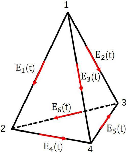
Figure 2. Electric field distribution of edges of the tetrahedral element.
Based on Galerkin’s weighted margin method and Eq. 5, the following equation can be obtained:
Finally, an equation in the following form is obtained:
where
where
where
In order to improve the numerical accuracy, the time is discretized using the second-order backward Euler difference scheme, and simultaneous Eq. 7 (Um et al., 2010):
Finally, large linear equations are formed, which can be expressed as follows:
In order to solve Eq. 13, the initial electric field
If the point source current strength is
where
The same grid is used to ensure the consistency of the boundary between the direct current electric field and the vector electric field, and the total field method is used to solve both the direct current (DC) field and the transient electromagnetic field. Due to the large solution area, the Dirichlet boundary condition is applied to the external boundary
The tangential electric fields of the edges of all of the tetrahedrons are obtained using the lower-upper (LU) decomposition and quick back substitution of the above equations using a multi-wavefront direct solver; namely, the multifrontal massively parallel sparse direct solver (MUMPS). The electric field response
To validate the accuracy of the algorithm proposed in this paper, a comparison verification is conducted using a homogeneous half-space model. Assuming that the resistivity of air is 106 Ω⋅m and the resistivity of the homogeneous half-space is 100 Ω⋅m, a vertical electric dipole with a depth range of 100 m–101 m underground is considered. The transmitting current is set to 1 A. The receiving point is located on the ground along the x-direction at a distance of 1,500 m from the transmitter. Schematic diagrams of the model and mesh partition are presented in Figure 3
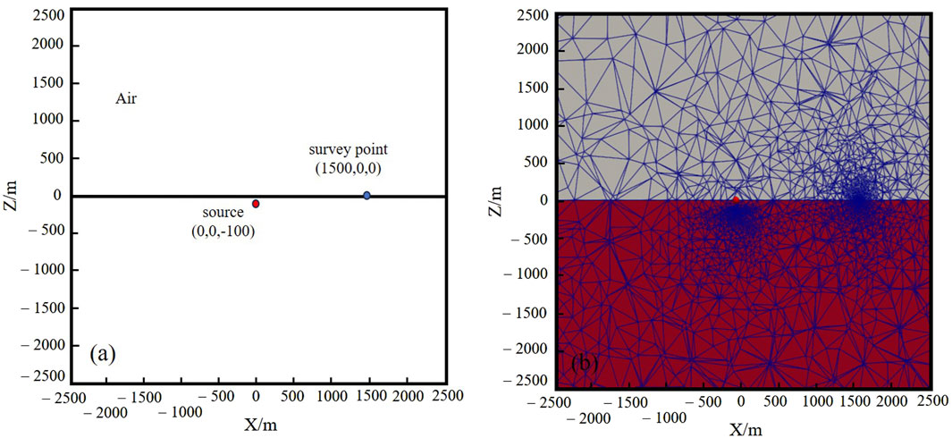
Figure 3. (A) Schematic diagram of the vertical electric dipole model in a uniform half-space, and (B) schematic diagram of its mesh discretization.
The computational results of the homogeneous half-space are compared and analyzed against the results obtained using COMSOL (Zheng and Zhao, 2023). As shown in Figure 4, the finite element solution closely matches the curve obtained using COMSOL. Based on calculations, the relative error between the two is within ±5%. Therefore, it can be concluded that the algorithm proposed in this paper is reliable and trustworthy.

Figure 4. (A) Comparison of the electric field results of the vertical electric dipoles in a uniform half space and (B) the relative error.
To verify the computational accuracy of the algorithm for complex geoelectric models, a three-dimensional model (Liu Y. J. et al., 2020) is designed. The electrical source has a length of 1,000 m, is arranged along the y-direction, and its center point is located at the surface (0,0,0). The transmitting current is set to 1 A. Three measurement points are arranged along the x-direction, and they have coordinates of A (−500,0,0), B (−1050,0,0), and C (−2000,0,0). Local refinement is applied to the mesh at the transmitter and measurement points (Figure 5).
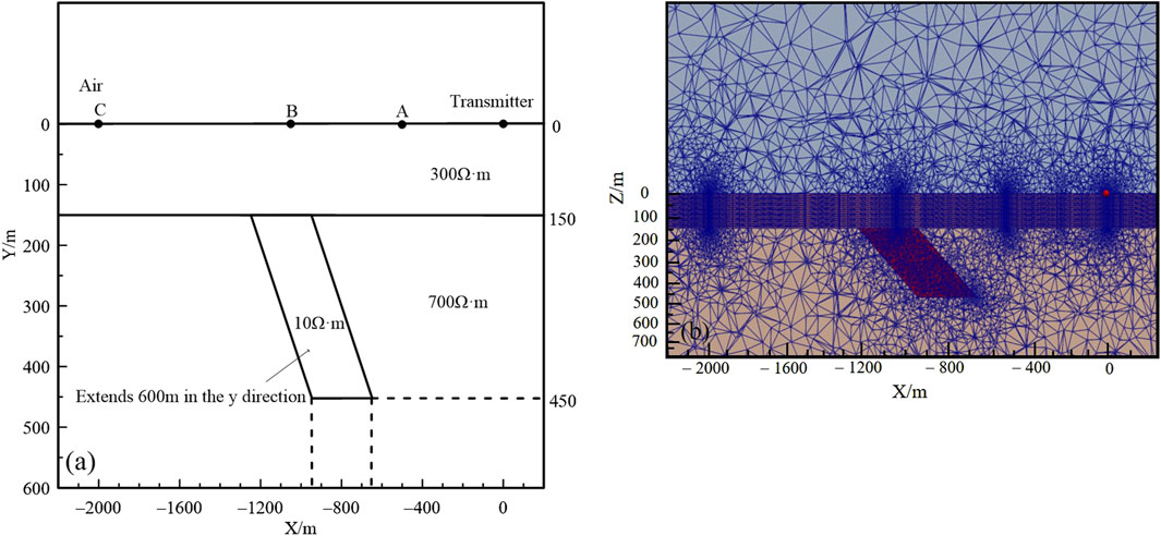
Figure 5. (A) Section diagram of a three-dimensional complex model and (B) schematic diagram of its mesh discretization.
Figure 6 compares the numerical results of the electric field component Ey at the three measurement points with the finite volume calculation results of Liu et al. (Liu Y. J. et al., 2020). It can be observed from Figure 6 that the results fit well, with errors all less than 5%. This demonstrates the accuracy of the algorithm proposed in this paper.
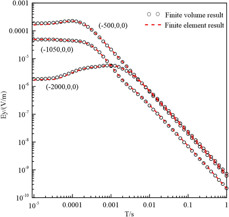
Figure 6. Results of the Ey component of the 3-D model in ground mode.
To theoretically explore the capability of the borehole transient electromagnetic method for the dynamic monitoring of shale gas hydraulic fracturing, a three-dimensional model (Figure 7) is designed. In this model, a layer of shale with a thickness of 300 m and resistivity of 40 Ω·m is located 2000 m below sea level. Above the shale layer, there is limestone with a thickness of 700 m and a resistivity of 2000 Ω·m, as well as mudstone with a thickness of 1,300 m and resistivity of 100 Ω·m. Below the shale layer, a layer of limestone with a resistivity of 2000 Ω·m and thickness of 4,300 m overlies a limestone substrate with a resistivity of 1,000 Ω·m. The wellhead is located at (0,0), where a transmitting source with a length of 2000 m along the z-direction is deployed. The transmitting current is set to 1 A. The measurement points are distributed within an x range of 200 m–5,000 m and a y range of −1,500 m–1,500 m, with a mesh size of 200 m × 200 m. Two hydraulic fracturing stages are conducted within the shale layer, each with a fracture range of 1,200 m × 1,000 m × 300 m. After fracturing, the resistivity changes to 5 Ω·m. Three observations are made at the surface to observe the response of the electric field before hydraulic fracturing, after the first fracturing stage, and after the second fracturing stage. The radial electric field
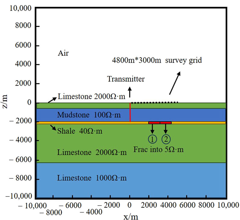
Figure 7. Schematic diagram of the shale fracturing model.
Figure 8 shows the
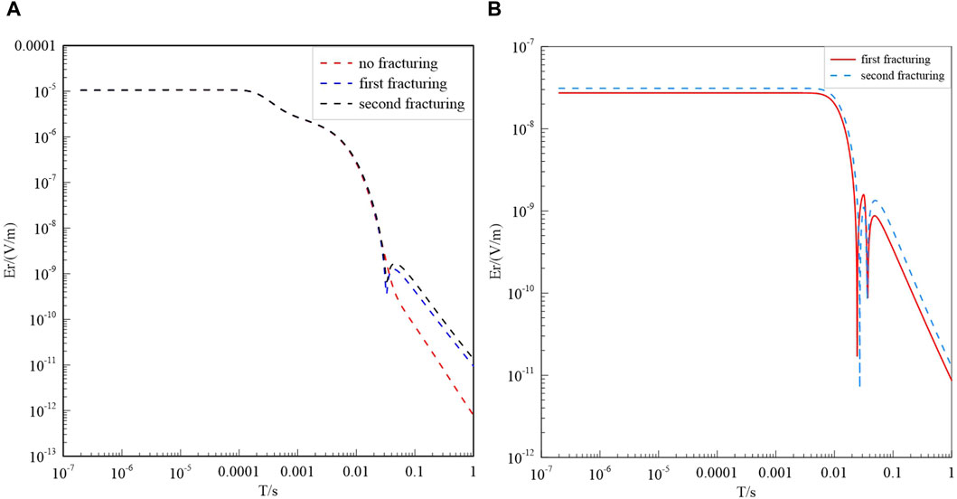
Figure 8. (A) Er response curve observed at the observation point (2200, 300, 0) at three times, and (B) the difference in Er between the first and second stages of fracturing and before fracturing.
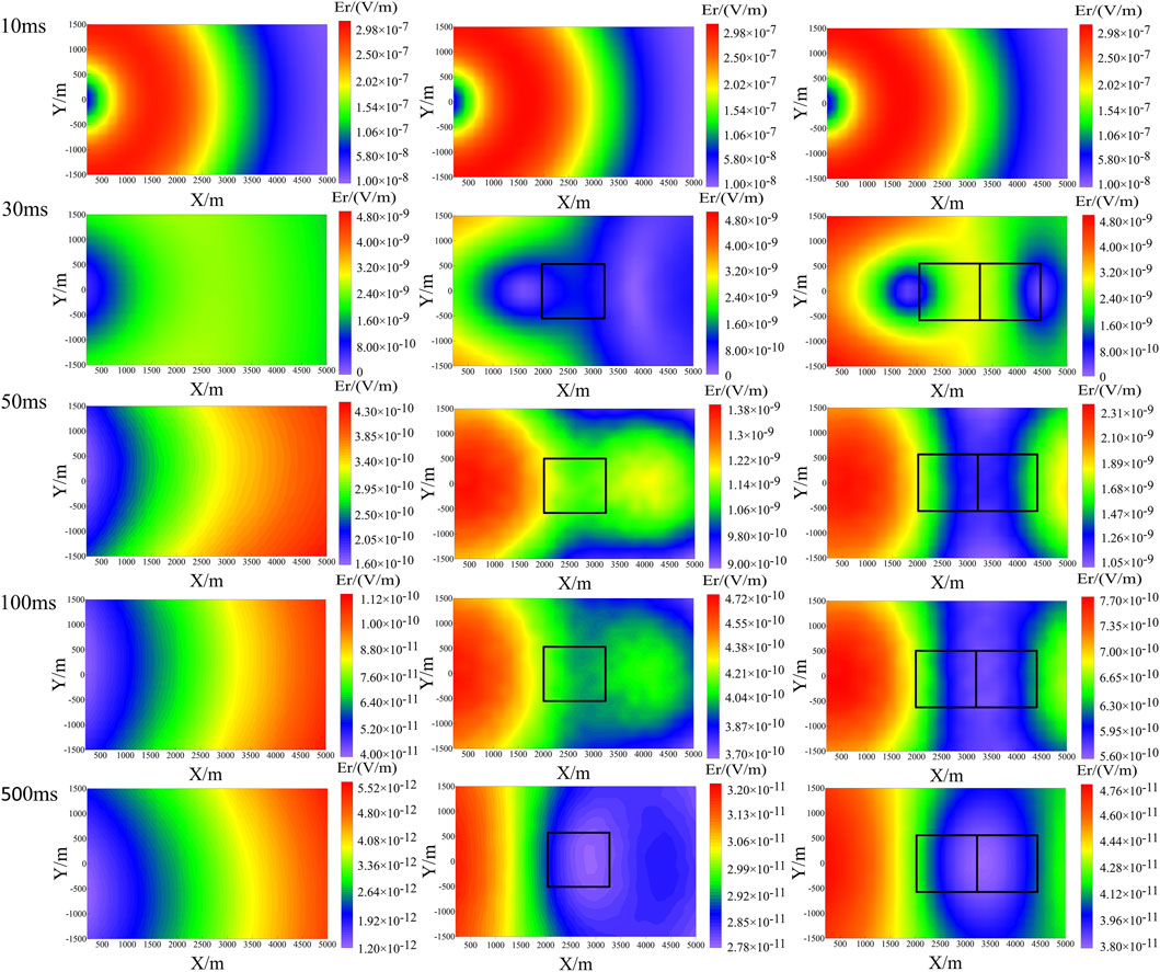
Figure 9. Response profiles of the electric field Er at 10 ms, 30 ms, 50 ms, 100 ms, and 500 ms, (rows one through five, respectively), and the response in the pre-fracturing, first-stage fracturing, and second-stage fracturing periods (columns one through three, respectively).
Figure 9 displays the response profiles of the electric field
To further analyze the changes in the electric field response values before and after hydraulic fracturing and to verify the applicability of this method in the dynamic monitoring of shale gas fracturing, we created difference profile maps of the electric field response
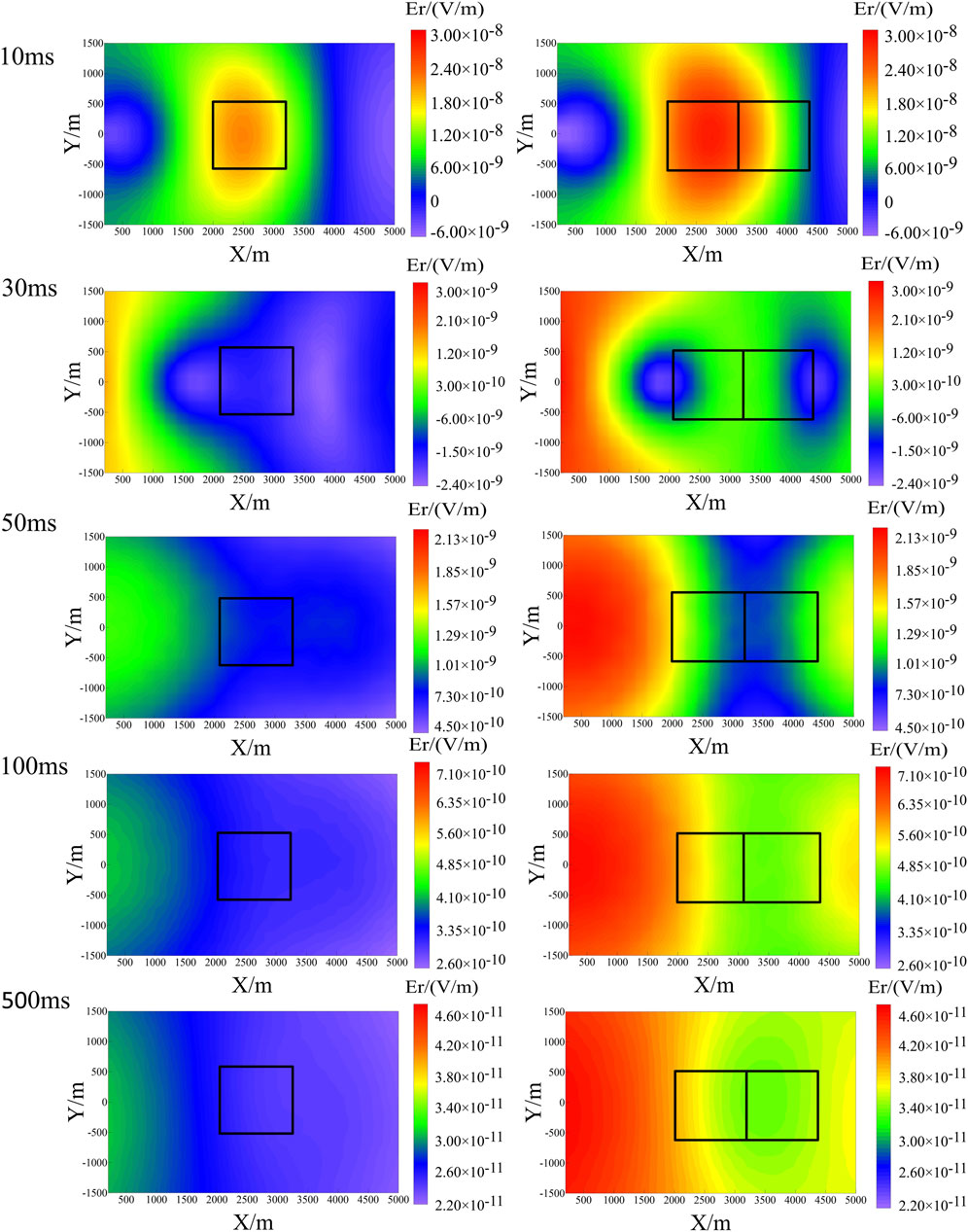
Figure 10. Response profiles of the electric field Er fracturing differential value in the first stage (column one) and second stage (column two) of Er fracturing at 10 ms, 30 ms, 50 ms, 100 ms, and 500 ms (rows one through five, respectively).
In this study, we applied the unstructured vector finite element method to three-dimensional forward simulation of the borehole transient electromagnetic (TEM) method for the dynamic monitoring of shale gas fracturing. The effectiveness of the borehole TEM method in monitoring the dynamic changes in underground mineral deposits and oil and gas reservoirs with resistivity differences was demonstrated. Based on the analysis of the response, the following conclusions were attained:
(1) Under the condition of a homogeneous half-space, the algorithm’s correctness was verified by comparing the finite element solution proposed in this study with the COMSOL solution. To further validate the accuracy of the algorithm, comparisons were made with the finite volume method in surface mode. It was demonstrated that the algorithm can effectively perform three-dimensional forward simulations of the borehole TEM method in complex models.
(2) Numerical analysis of underground shale gas reservoir models revealed that the borehole TEM method can effectively characterize the electrical differences before and after shale gas fracturing, thereby achieving high-precision dynamic monitoring of shale gas fracturing.
At present, many scholars have carried out the research of borehole to ground transient electromagnetic method, but it is rarely applied to the dynamic monitoring of shale gas fracturing. With the help of this algorithm proposed in this study allows for the analysis of the patterns of the borehole TEM method in the dynamic monitoring of unconventional oil and gas fracturing. This provides theoretical guidance for the dynamic monitoring of unconventional oil and gas fracturing in practical production processes.
The original contributions presented in the study are included in the article/Supplementary Material, further inquiries can be directed to the corresponding author.
WZ: Conceptualization, Formal Analysis, Methodology, Software, Writing–original draft. XX: Conceptualization, Methodology, Resources, Writing–review and editing. LZ: Formal Analysis, Resources, Writing–review and editing. XW: Software, Validation, Writing–review and editing. LY: Supervision, Writing–review and editing.
The author(s) declare that financial support was received for the research, authorship, and/or publication of this article. This research was funded by the National Natural Science Foundation of Key Project of China, grant number 42030805; the National Natural Science Foundation of China, grant number 42274103; and the Science and Technology Department Project of China Petroleum & Chemical Corporation, grant number P22163.
The authors declare that the research was conducted in the absence of any commercial or financial relationships that could be construed as a potential conflict of interest.
The authors declare that they have no known competing financial interests or personal relationships that could have appeared to influence the work reported in this paper.
All claims expressed in this article are solely those of the authors and do not necessarily represent those of their affiliated organizations, or those of the publisher, the editors and the reviewers. Any product that may be evaluated in this article, or claim that may be made by its manufacturer, is not guaranteed or endorsed by the publisher.
Ansari, S., and Farquharson, C. G. (2014). 3D finite–element forward modeling of electromagnetic data using vector and scalar potentials and unstructured grids. Geophysics 79, 149–165. doi:10.1190/geo2013-0172.1
Commer, M., Helwig, S. L., Hördt, A., Scholl, C., and Tezkan, B. (2006). New results on the resistivity structure of Merapi Volcano (Indonesia), derived from three-dimensional restricted in version of long-offset transient electromagnetic data. Geophys. J. Int. 167, 1172–1187. doi:10.1111/j.1365-246x.2006.03182.x
Cuevas, N. (2012). “Casing effect in borehole-surface (surface-borehole) EM fields,” in 74th Annual International Conference and Exhibition, EAGE//Extended Abstracts, P201.
Ghada, M. S., and Al-Najim, F. A. (2015). The transient electromagnetic field created by electric line source on a plane conducting Earth. Int. J. Mech. Appl. 5, 16–22. doi:10.5923/j.mechanics.20150501.03
Haroon, A., Adrian, J., Bergers, R., Gurk, M., Tezkan, B., Mammadov, A. L., et al. (2015). Joint inversion of long-offset and central-loop transient electromagnetic data: application to a mud volcano exploration in Perekishkul, Azerbaijan. Geophys. Prospect. 63, 478–494. doi:10.1111/1365-2478.12157
He, J. S., and Xue, G. Q. (2018). Review of the key techniques on short-offset electromagagnetic detection. Chin. J. Geophys. 61, 1–8. doi:10.6038/cig2018L0003
Hördt, A., Druskin, V. L., Knizhnerman, L. A., and Strack, K. M. (1992). Interpretation of 3-D effects in long-offset transient electromagnetic (LOTEM) soundings in the Münsterland area/Germany. Geophysics 57, 1127–1137. doi:10.1190/1.1443327
Hu, W. B., Shen, J. S., and Yan, L. J. (2022). Principle and application of controllable source electromagnetic method for reservoir fluid prediction. China: Science Press.
Hu, Z. Z., He, Z. X., Li, D. C., Liu, Y. X., Sun, W. B., Wang, C. F., et al. (2014). Reservoir monitoring feasibility study with time lapse magnetotellurics survey in Sebei Gas Field. Oil Geophys. Prospect. 49, 997–1005. doi:10.13810/j.cnki.issn.1000-7210.2014.05.051
Ke, G. P., and Huang, Q. H. (2009). 3D forward and inversion problems of borehole-to-surface electrical method. Acta Sci. Nat. Univ. Pekin. 45, 264–272. doi:10.13209/j.0479-8023.2009.041
Keller, G. V., Pritchard, J. I., Jacobson, J. J., and Harthill, N. (1984). Megasource time-domain electromagnetic sounding methods. Geophysics 49, 993–1009. doi:10.1190/1.1441743
Li, J. H., He, Z. X., and Xu, Y. X. (2017). Three-dimensional numerical modeling of surface-to-borehole electromagnetic method for monitoring reservoir. Appl. Geo-physics 14, 101–111. doi:10.1007/s11770-017-0643-8
Liu, R., Liu, J., Wang, J., Liu, Z., and Guo, R. W. (2020a). A time-lapse CSEM monitoring study for hydraulic fracturing in shale gas reservoir. Mar. Petroleum Geol. 120, 104545. doi:10.1016/j.marpetgeo.2020.104545
Liu, Y. J., Yogeshwar, P., Hu, X. Y., Peng, R. H., Tezkan, B., Mörbe, W., et al. (2020b). Effects of electrical anisotropy on long-offset transient electromagnetic data. Geophys. J. Int. 222, 1074–1089. doi:10.1093/gji/ggaa213
Mitsuhata, Y. J., Uchida, T., and Amano, H. (2002). 2.5-D in-version of frequency-domain electromagnetic data generated by a grounded-wire source. Geophysics 67, 1753–1768. doi:10.1190/1.1527076
Müller, M., Hördt, A., and Neubauer, F. (2002). Internal structure of Mount Merapi, Indonesia, derived from long-offset transient electromagnetic data. J. Geophys. Res. Solid Earth 107. doi:10.1029/2001jb000148
Orange, A., Key, K., and Constable, S. (2009). The feasibility of reservoir monitoring using time-lapse marine CSEM. Geophysics 74, 21–29. doi:10.1190/1.3059600
Peng, R. H., Hu, X. Y., Liu, Y. X., and He, Z. X. (2012). “The feasibility study of time-lapse two dimensional magnetotelluric for reservoir monitoring,” in The 28th Annual Meeting of the Chinese Geophysical Society, Beijing, China.
Strack, K. M. (1984). The deep transient electromagnetic sounding technique: first field test in Australia. Explor. Geophys. 15, 251–259. doi:10.1071/eg984251
Um, E. S., Harris, J. M., and Alumbaugh, D. L. (2010). 3D time–domain simulation of electromagnetic diffusion phenomena: a finite–element electric–field approach. Geophysics 75, 115–126. doi:10.1190/1.3473694
Wang, X. Y., Yan, L. J., and Mao, Y. R. (2022). Simulation and analysis of dynamic monitoring of oil and gas reservoir based on grounded electric source TEM. Oil Geophys. Prospect. 57, 459–466. doi:10.13810/j.cnki.issn.1000-7210.2022.02.023
Wang, Z. G., He, Z. X., and Liu, Y. (2006). Research of three-dimension modeling and anomalous rule on borehole-ground DC method. Chin. J. Eng. Geophys. 3, 87–92.
Wang, Z. G., He, Z. X., and Wei, W. B. (2007). Research on 3D modeling of borehole vertical bipole using body integral equation. Prog. Geophys. 22, 1802–1808.
Wirianto, M., Mulder, W. A., and Slob, E. C. (2010). A feasibility study of land CSEM reservoir monitoring in a complex 3-D model. Geophys. J. Interna-tional 181, 741–755. doi:10.1111/j.1365-246x.2010.04544.x
Xie, X. B., Zhou, L., Yan, L. J., and Hu, W. B. (2016). Remaining oil detection with time-lapse long offset& window transient electromagnetic sounding. Oil Geophys. Prospect. 51, 605–612. doi:10.13810/j.cnki.issn.1000-7210.2016.03024
Zhang, J. Q. (2018). Finite-length wire Source3D electromagnetic forward modeling of vertical. Beijing, China: China University of Geosciences.
Zhao, P. Q., Hao, H. M., Ni, T. L., Li, H. G., Tao, Z. Q., and Ma, Y. H. (2019). A novel technology: reservoir seepage geophysics. Oil Geophys. Prospect. 54, 719–728. doi:10.13810/j.cnki.issn.1000-7210.2019.03.028
Keywords: borehole transient electromagnetic method, finite element, three-dimensional forward modeling, dynamic monitoring, shale gas fracturing
Citation: Zhang W, Xie X, Zhou L, Wang X and Yan L (2024) 3-D forward modeling of shale gas fracturing dynamic monitoring using the borehole-to-ground transient electromagnetic method. Front. Earth Sci. 12:1394094. doi: 10.3389/feart.2024.1394094
Received: 01 March 2024; Accepted: 21 March 2024;
Published: 09 April 2024.
Edited by:
Wenguang Wang, Northeast Petroleum University, ChinaCopyright © 2024 Zhang, Xie, Zhou, Wang and Yan. This is an open-access article distributed under the terms of the Creative Commons Attribution License (CC BY). The use, distribution or reproduction in other forums is permitted, provided the original author(s) and the copyright owner(s) are credited and that the original publication in this journal is cited, in accordance with accepted academic practice. No use, distribution or reproduction is permitted which does not comply with these terms.
*Correspondence: Lei Zhou, 501161@yangtzeu.edu.cn
Disclaimer: All claims expressed in this article are solely those of the authors and do not necessarily represent those of their affiliated organizations, or those of the publisher, the editors and the reviewers. Any product that may be evaluated in this article or claim that may be made by its manufacturer is not guaranteed or endorsed by the publisher.
Research integrity at Frontiers
Learn more about the work of our research integrity team to safeguard the quality of each article we publish.