Grounded source transient electromagnetic 3D forward modeling with the spectral-element method and its application in hydraulic fracturing monitoring

A long wire with large current source transient electromagnetic (TEM) monitoring, with a large detection depth, low cost, safety, and environmental protection, has unique advantages in the testing and identification of unconventional reservoir fluid and the evaluation of stimulated reservoir volume. So, the TEM 3D forward modeling method has become a research hotspot. Although the finite-element method (FEM) is a type of numerical algorithm that has been widely applied in three-dimensional (3D) electromagnetic field forward modeling, the efficiency and accuracy of FEM require further improvement in order to meet the demand of fast 3D inversion. By increasing the order of the basis function and adjusting the principle of mesh discretization, the precision of the mixed-order spectral-element (SEM) result will be increased. The backward Euler scheme is an unconditionally stable technique which can ignore the impact of the scale of the time step. To achieve a better description of the nonlinear electromagnetic (EM) response of the grounded source TEM method and to optimize the efficiency and accuracy/precision of the 3D TEM forward modeling method significantly, we proposed the use of 3D TEM forward modeling based on the mixed-order SEM and the backward Euler scheme, which can obtain more accurate EM results with fewer degrees of freedom. To check its accuracy and efficiency, the 1D and 3D layered models are applied to compare the SEM results with the semi-analytical and FEM solutions. In addition, we analyzed the accuracy and efficiency of the SEM method for different types of order basis functions. Finally, we calculated the long-wire source TEM response for a practical 3D earth model of a shale gas reservoir for fracturing monitoring and tested the feasibility of the TEM method in a hydraulic fracturing monitoring area to further demonstrate the flexibility of the SEM method.

Highlights

This paper achieved long-wire source TEM-efficient and high-precision forward modeling for a practical 3D earth model of a shale gas reservoir for fracturing monitoring based on the SEM method, which verified the feasibility of the long-wire source TEM method in a hydraulic fracturing monitoring area, and further demonstrated the flexibility of SEM.

This paper proposed the use of 3D grounded source TEM forward modeling based on SEM and the backward Euler scheme, which can obtain more accurate EM results with fewer degrees of freedom.

This paper verified the accuracy and efficiency of the 3D long-wire source grounded source TEM via SEM, in which the lower-order spectral-element method with a detailed mesh and the higher-order spectral-element method with a coarse mesh have similar precision levels.

Introduction

Due to the rise and development in the field of hydraulic fracturing key technologies, significant progress has been made in the exploration and development of unconventional reservoir resources. Hydraulic fracturing technology injects fracturing fluid and proppants into the wellbore, which generates an artificial dense fractured network, and improves fluid transport channels, fracture development modes, and properties of unconventional reservoirs, thereby realizing the stimulated reservoir volume (SRV) modification. Hydraulic fracturing is an essential technical method in unconventional oil and gas development, and hydraulic fracturing monitoring is the key technique for accurately evaluating the effect of hydraulic fracturing and reservoir transformation. SRV is crucial for optimizing the well completion strategy, resource utilization, and reservoir productivity prediction. The reservoir physical property is a critical technology for SRV prediction and evaluation, and it has significant implications for optimizing fracturing construction and reducing costs. Time-lapse seismicity is the primary means of monitoring fracturing (Ahmadian et al., 2018). However, the micro-seismic method infers the location of fracturing by recording seismic events caused by rock fractures or sliding in the reservoir, including the positions of fracturing failure, in which effective support is not achieved after pressure loss. Thus, it may limit the development of fine-grained fracturing monitoring technologies. Fortunately, a low-resistance, high-polarization electromagnetic (EM) anomaly is formed in the reservoir regions with the fracturing fluid injected, which differs significantly from the surrounding rocks in electrical properties. Thus, EM monitoring has unique advantages in identifying fluid characteristics compared to the micro-seismic method (Strack, 2014). With the improvement of instrument equipment and data acquisition technology, the time-lapse EM monitoring technology is becoming increasingly mature and has become a research hotspot for unconventional reservoir monitoring. EM exploration methods, such as magnetotelluric (MT) and controlled-source electromagnetic (CSEM) methods, have been widely applied in the field of fracturing monitoring (Streich, 2016). Subsequently, the MT method has received more attention in deep geothermal hydraulic fracturing monitoring (Peacock et al., 2012; Peacock et al., 2013; Abdallah et al., 2020). The MT method is more suitable for monitoring hydraulic fracturing in large-scale and deep reservoirs. The CSEM method has a high sensitivity to thin layers, which promotes the application of the CSEM method in unconventional reservoir identification (Tietze et al., 2015; Liu R. et al., 2020).

It must be admitted that a large part of the unconventional oil and gas reservoirs are located in areas with complicated topography and geological conditions, which pose higher requirements on the resolution, exploration depth, and data processing and interpretation of EM hydraulic fracturing monitoring. The high-power and long-wire source transient electromagnetic method (TEM) has obvious advantages, such as a high signal-to-noise ratio, large exploration depth, and low cost. It is considered one of the most effective methods for monitoring hydraulic fracturing in unconventional reservoirs for complicated topography and geological conditions, especially compared to the conventional reservoir EM method (such as MT and CSEM) with time-lapse monitoring (Hördt et al., 1992; Schamper et al., 2011; Yan et al., 2018; Di et al., 2019; Liu Y. et al., 2020). The 3D forward modeling of time-domain EM induction is aimed at calculating the EM responses and variations at different stages of hydraulic fracturing, which is an important basis for the feasibility analysis and scheme design of dynamic monitoring (Orange et al., 2009). Ceia et al. (2007) demonstrated the effectiveness of long wire with large current TEM monitoring through 1D simulation. However, 1D modeling is based on the assumption of horizontally extended layered models, which is seriously inconsistent with the limited horizontal variation in the hydraulic fracturing area. Therefore, in order to obtain accurate responses to dynamic hydraulic fracturing changes, it is necessary to develop 3D forward modeling for complex models (Peacock et al., 2013; Didana et al., 2017).

There are two types of 3D TEM forward modeling schemes: indirect and direct methods. The indirect method utilizes the inverse Fourier transform method and 3D frequency-domain electromagnetic (EM) modeling simultaneously, which applies a numerical method, such as the integral equation method, finite-difference method (FDM), and finite-element method (FEM), to calculate the frequency-domain EM response. Then, the frequency domain can be converted to the time-domain response by the inverse Fourier transform (Mulder et al., 2008). Cox et al. (2012) calculated the time-domain EM response and sensitivity matrix by the integral equation method and the cosine transform. Sasaki et al. (2015) proposed a time-domain EM data inversion method on the strength of the inverse Fourier transform and frequency-domain FDM forward modeling, and they tested the inversion efficiency for practical data. Regarding the direct algorithm, it is derived from the time-domain governing equations, and space and time discretizations are conducted directly via a numerical method, including explicit and implicit schemes. The explicit scheme generally utilizes the central difference for time discretization. Commer and Newman (2004) used the finite-difference time-domain (FDTD) method based on a staggered grid and the modified Dufort–Frankel method to obtain a parallel algorithm for electrical source 3D TEM forward modeling, which effectively improved the modeling efficiency. Based on this, Commer et al. (2015) carried out the 3D TEM forward modeling of a drill steel casing method and developed a time-dependent function in the Dufort–Frankel method, which reduces the computation cost by using a larger time step. The implicit scheme adopts the backward difference method for time discretization. Um et al. (2010) realized electrical source 3D TME forward modeling based on unstructured grid FEM and the backward Euler technique and improved the modeling accuracy by the adaptive time-step method, which significantly promoted the application of the implicit method in 3D TEM modeling. Liu R. et al. (2020) combined the finite volume method and the backward Euler technique with second order to realize 3D long offset TEM forward modeling of arbitrary anisotropic media and analyzed the anisotropic anomaly response characteristics for typical geological models. Li et al. (2020) discussed the characteristics of the semi-airborne electrical source TEM response based on FEM and analyzed the impact of fluctuating terrain on the EM response using practical geological models. Based on unstructured grid FEM and the implicit scheme, Wang et al. (2021) achieved surface-to-borehole 3D TEM forward modeling and studied the resolution of surface-to-borehole TEM for anomalous targets. Lu et al. (2021) developed 3D TEM forward modeling codes using the unstructured grid finite volume method and the implicit scheme, proposed a trial-and-error modeling approach, and tested the practicability.

However, their methodology requires the EM response of a large number of frequency points be calculated for the indirect method, which limits the calculation efficiency and accuracy. The time and spatial step sizes have serious impacts on the precision and computational efficiency of the explicit method. The implicit method has the significant advantage of unconditional stability. However, the implicit method requires that large linear equations be solved in each time step, and this inherent property limited the application of the implicit method in early 3D forward modeling applications. With the rapid development of large, sparse direct solvers, the implicit method has become widely used for 3D TEM forward modeling. In particular, the combination of FEM and the backward Euler scheme, which has the advantages of flexible modeling and unconditional stability, is now broadly applied in 3D TEM forward modeling. However, the distribution of the EM field in a discrete element is normally assumed as a linear function or constant, which is inconsistent with real EM response characteristics. Therefore, it is an essential factor in 3D forward modeling to obtain a balance between accuracy and efficiency.

As a combination of the spectral method and traditional first-order FEM, the spectral-element method (SEM) has the characteristics of exponential convergence of the spectral method and flexible modeling of FEM. Thus, it can fit more complex models and has the advantage of synchronized optimization of the accuracy and efficiency for the targets. Compared with FEM, SEM introduces high-order polynomials as the interpolation basis function, which can enhance the interpolation accuracy and effectively improves the modeling efficiency and accuracy. Patera (1984) first proposed to utilize the Gauss–Lobatto–Chebyshev (GLC) polynomial as the basis function of SEM, and then, this method was applied to the numerical simulation of fluid mechanics. Later, Røquist and Patera (1987) proposed an alternative type of SEM, in which the basis function was formed by Gauss–Lobatto–Legendre (GLL) polynomials. The aforementioned basis functions have become the two most common types of SEMs. Since then, SEM has been developing rapidly and is widely used in seismic exploration (Komatitsch et al., 1999; Boaga et al., 2012; Liu et al., 2014; Gharti et al., 2019; Khan et al., 2020). In the 21st century, SEM is gradually applied in the field of computational EM and has been applied in micro-wave and circuit simulation research (Cohen, 2003; Lee and Liu, 2004; Lu and Li, 2007). Referring to the application of SEM in computational EM, researchers are trying to apply SEM to geophysical EM forward modeling. Zhou et al. (2016); Zhou et al. (2017) introduced SEM for the forward modeling of 3D frequency-domain CSEM. Based on the GLL basis function, Huang et al. (2017); Huang et al. (2019) realized the forward modeling of 3D airborne EM infrequency domain and time domain separately. Based on the GLC basis function, Zhu et al. (2020), 2022) applied the unstructured tetrahedral grid SEM to 3D direct current resistivity and frequency-domain airborne EM forward modeling and analyzed the modeling accuracy and efficiency of this method. Therefore, the efficiency and accuracy of SEM in geophysical EM modeling have been continuously verified. However, few studies have been conducted on 3D long-wire source TEM forward modeling using SEM. Therefore, we conduct research to realize 3D TEM forward modeling by SEM.

Based on the GLL interpolation basis function, in order to discretize the time-domain electric field diffusion equation, the Galerkin weighted residual method was introduced. Using an electric dipole to approximate the grounding of a long conductor source, combined with the second-order backward Euler technique and parallel direct solution technology, the high-efficiency and high-precision 3D forward modeling of electrical source TEM was realized, and the application effect of SEM in this field was tested. The stability of the algorithm was tested on 1D and 3D models, and then, the feasibility of applying the electrical source transient electromagnetic method in shale gas reservoir fracturing dynamic monitoring was analyzed. First, we derived the discretization formula from the time-domain Maxwell equation. We used the GLL basis function to discretize the EM field and the Galerkin weighted residual method to establish spatial discretization equations. Then, the implicit backward Euler scheme was introduced for temporal dispersion. In addition, to obtain a fast and accurate EM response, we applied the rational piecewise functional type of the electrical dipole to approximate the long-wire source, and we applied the direct parallel solver to accelerate the solution. Next, we verified the accuracy of SEM for layer-earth and 3D earth models and compared the results with those of the semi-analytical solution and FEM. We also investigated the influence of the basis function order on the modeling results. Finally, to further test the flexibility and adaptability of our method for complex earth models, we set a practical hydraulic fracturing monitoring earth model with small-scale targets and a large burial depth, and we analyzed the feasibility of applying long-wire source TEM to shale gas reservoir fracturing monitoring.

Over the last decade, forward modeling tests and EM techniques have been gradually introduced for hydraulic fracturing monitoring (Tietze et al., 2019). For frequency-domain EM methods, Bhuyian et al. (2012) and Zhdanov et al. (2013) first applied magnetotelluric (MT) and controlled-source electromagnetic (CSEM) data for hydraulic fracturing monitoring and proved the applicability of the reservoirs within a depth of 2 km. Tietze et al. (2015) studied the sensitivity of the CSEM method and concluded that by borehole-to-surface configuration, the EM signal changes caused by the hydraulic fracturing reservoir at the depth of 1200 m can be captured. Strack (2010) compared the detection capability between the MT and time-domain CSEM methods, and proposed that the time-domain CSEM method has a better resolution for reservoir monitoring. In the field study of a petroleum field in Brazil, Ceia et al. (2007) used 1D forward modeling and inversion to interpret the TEM signals of the long-wire source EM method and proved that this method can monitor fluid dynamic changes at a depth of 1 km.

In this paper, we proposed the use of 3D TEM forward modeling based on the mixed-order SEM and the backward Euler scheme. First, we derived the theoretical equations for the grounded source TEM 3D forward modeling with spatial discretization based on SEM and temporal discretization based on the backward Euler scheme. In addition, to effectively suppress the singularity caused by the source, we applied the rational piecewise functional type of the electrical dipole to approximate the long-wire source. Then, we adopted a direct solver to accelerate the solution of the SEM discrete equations. Moreover, to check its accuracy and efficiency, the 1D and 3D layered models are applied to compare the SEM results with the semi-analytical and FEM solutions. In addition, we analyzed the accuracy and efficiency of the SEM method for different types of order basis functions. Finally, we calculated the long-wire source TEM response for a practical 3D earth model of a shale gas reservoir for fracturing monitoring and tested the feasibility of the TEM method in a hydraulic fracturing monitoring area to further demonstrate the flexibility of the SEM method.

Methodology

Governing equations and initial–boundary conditions

Without considering the displacement current, we can derive the following electric field diffusion equation of time domain easily.

$\nabla \times \left[\frac{1}{\mu }\nabla \times \mathit{E}\right]+\sigma \frac{\partial \mathit{E}}{\partial t}+\frac{\partial {\mathit{J}}_{\mathrm{s}}}{\partial t}=0.(1)$

To avoid multi-solutions of the EM field, the boundary and initial conditions are needed for solving the EM diffusion problem. For the boundary condition, we adopt a finite and large-scale 3D region with a boundary surface $\mathrm{\Gamma }$ to replace the infinite 3D modeling region. Hence, on the boundary, the tangential component of the electrical field will be reduced to zero, and thus, the following Dirichlet boundary condition will hold.

${\left.\left(\mathbf{n}\times \mathbf{E}\right)\right|}_{\mathrm{\Gamma }}=0,(2)$

where $\mathbf{n}$ is the out normal direction of the outer boundary. Moreover, the initial electric field is set as 0 for a full waveform current source. As for a step-off source, a stable direct current electric field is set as the initial electric field, which can be obtained by solving the Poisson equation (Commer and Newman, 2004).

Space discretization for SEM

We use the hexahedral element to discretize the geoelectrical underground model and apply the mixed-order SEM to conduct spatial discretization. Then, the interpolated electric field can be expressed as follows (Huang et al., 2019):

$\begin{array}{l}\mathit{E}\left(x,y,z,t\right)={\displaystyle \sum _{k=0}^{N_z}}{\displaystyle \sum _{s=0}^{N_y}}{\displaystyle \sum _{r=0}^{N_x-1}}{E}_x\left(x_r,y_s,z_k,t\right){\stackrel{\sim }{\mathit{\Phi }}}_{rsk}^x\\ +{\displaystyle \sum _{k=0}^{N_z}}{\displaystyle \sum _{s=0}^{N_y-1}}{\displaystyle \sum _{r=0}^{N_x}}{E}_y\left(x_r,y_s,z_k,t\right){\stackrel{\sim }{\mathit{\Phi }}}_{rsk}^y\\ +{\displaystyle \sum _{k=0}^{N_z-1}}{\displaystyle \sum _{s=0}^{N_y}}{\displaystyle \sum _{r=0}^{N_x}}{E}_z\left(x_r,y_s,z_k,t\right){\stackrel{\sim }{\mathit{\Phi }}}_{rsk}^z\\ ={\displaystyle \sum _{i=0}^{Ne}}{E}_i\left(x_r,y_s,z_k,t\right){\stackrel{\sim }{\mathit{\Phi }}}_i,\end{array}(3)$

where $\stackrel{\sim }{\mathit{\Phi }}=\left[{\stackrel{\sim }{\mathit{\Phi }}}^x,{\stackrel{\sim }{\mathit{\Phi }}}^y,{\stackrel{\sim }{\mathit{\Phi }}}^z\right]$ is the physical domain basis function, and $N_x$, $N_y$, and $N_z$ are separately the basis function orders along each axis. $Ne=N_x\left(N_y+1\right)\left(N_z+1\right)+N_y\left(N_x+1\right)\left(N_z+1\right)+N_z\left(N_x+1\right)\left(N_y+1\right)$ is the number of total edges for the physical elements, and $E_i\left(x_r,y_s,z_k,t\right)$ and ${\stackrel{\sim }{\mathit{\Phi }}}_i$ are the tangential electric field and basis function on the ith total edge, respectively. Figure 1 presents a schematic diagram of a third-order SEM element ($N_x=3$, $N_y=3$ , and $N_z=3$).

FIGURE 1

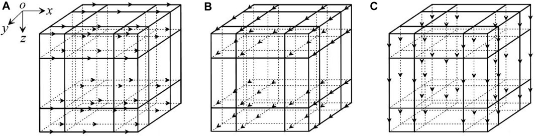
FIGURE 1. Schematic diagram of a third-order SEM element ($N_x=3$, $N_y=3$, and $N_z=3$): (A) edge elements along the x-axis; (B) edge elements along the y-axis; and (C) edge elements along the z-axis.

We apply the Galerkin method to minimize the weak form of Eq. 1, and we introduce the first vector Green’s theorem and Dirichlet boundary conditions. For all of the discrete elements,

$\begin{array}{l}{\displaystyle \sum _{e=1}^K}{\displaystyle \sum _{i,j=1}^{Ne}}{E}_j\frac{1}{\mu }{{\iiint }_{{\mathrm{\Omega }}^e}\left(\nabla \times {\stackrel{\sim }{\mathit{\Phi }}}_i\right)}^{\mathrm{T}}\cdot \left(\nabla \times {\stackrel{\sim }{\mathit{\Phi }}}_j\right)\mathrm{d}V+{\displaystyle \sum _{e=1}^K}{\displaystyle \sum _{i,j=1}^{Ne}}\frac{\mathrm{d}{E}_j}{\mathrm{d}t}\sigma {\iiint }_{{\mathrm{\Omega }}^e}{{\stackrel{\sim }{\mathit{\Phi }}}_i}^{\mathrm{T}}\cdot {\stackrel{\sim }{\mathit{\Phi }}}_j\mathrm{d}V\\ =-{\displaystyle \sum _{e=1}^K}{\displaystyle \sum _{i=1}^{Ne}}{\iiint }_{{\mathrm{\Omega }}^e}{{\stackrel{\sim }{\mathit{\Phi }}}_i}^{\mathrm{T}}\cdot \frac{\partial {\mathit{J}}_{\mathrm{s}}}{\partial t}\mathrm{d}V,\end{array}(4)$

where K represents the number of elements. Through element matrix analysis of SEM, we obtain

$\mathit{A}\mathit{E}+\mathit{B}\frac{\mathrm{d}\mathit{E}}{\mathrm{d}t}+\mathit{S}=0,(5)$

where $\mathit{A}$ is the total stiffness matrix, $\mathit{B}$ is the total mass matrix, $\mathit{S}$ is the imposed source vector, and $\mathit{E}$ is the electric field vector to be solved on the discrete edges.

Gauss–Lobatto–Chebyshev (GLC) and Gauss–Lobatto–Legendre (GLL) polynomials are generally introduced to form the basis function of SEM. The GLL-type basis function is more widely applied in EM simulation applications, and the 1D GLL-type basis function is expressed as follows:

${\phi }_j^{\left(N\right)}\left(\xi \right)=\frac{-1}{N\left(N+1\right)L_N\left({\xi }_j\right)}\frac{\left(1-{\xi }^2\right)}{\left(\xi -{\xi }_j\right)}{L}_N^{\prime }\left(\xi \right)j=1,\cdots ,N,(6)$

where $L_N\left(\xi \right)$ and $L_N^{\prime }\left(\xi \right)$ are the Nth order Legendre orthogonal polynomial and its derivative, respectively, and ${\xi }_j$ is the jth interpolation node of the GLL polynomial, which can be solved using $\left(1-{\xi }^2\right)L_N^{\prime }\left(\xi \right)=0$. Thus, the definition domain of the GLL polynomial is [−1,1]. Moreover, for mixed-order SEM, the 3D GLL basis function $\mathit{\Phi }=\left[{\mathit{\Phi }}^{\xi },{\mathit{\Phi }}^{\eta },{\mathit{\Phi }}^{\zeta }\right]$ can be derived by the 1D GLL polynomials in three orthogonal directions ($\xi$, $\eta$, and $\zeta$ directions) as follows:

${\mathit{\Phi }}_{rsk}^{\xi }\left(\xi \right)={\phi }_r^{\left(N_{\xi }-1\right)}\left(\xi \right){\phi }_s^{\left(N_{\eta }\right)}\left(\eta \right){\phi }_k^{\left(N_{\zeta }\right)}\left(\zeta \right)\cdot \overrightarrow{\xi },(7)$

${\mathit{\Phi }}_{rsk}^{\eta }\left(\eta \right)={\phi }_r^{\left(N_{\xi }\right)}\left(\xi \right){\phi }_s^{\left(N_{\eta }-1\right)}\left(\eta \right){\phi }_k^{\left(N_{\zeta }\right)}\left(\zeta \right)\cdot \overrightarrow{\eta },(8)$

${\mathit{\Phi }}_{rsk}^{\zeta }\left(\zeta \right)={\phi }_r^{\left(N_{\xi }\right)}\left(\xi \right){\phi }_s^{\left(N_{\eta }\right)}\left(\eta \right){\phi }_k^{\left(N_{\zeta }-1\right)}\left(\zeta \right)\cdot \overrightarrow{\zeta },(9)$

where $\overrightarrow{\xi }$, $\overrightarrow{\eta }$, and $\overrightarrow{\zeta }$ represent the corresponding unit vectors. The definition domain of the GLL-type 3D basis function is $\left(\xi ,\eta ,\zeta \right)\in \left[-\mathrm{1,1}\right]\times \left[-\mathrm{1,1}\right]\times \left[-\mathrm{1,1}\right]$. Similar to the basis function of vector FEM, the order of the polynomial in the tangential direction of the basis function of the mixed-order SEM is one order less than those in the normal direction. Thus, for the interface between two adjacent elements, the mixed-order basis function can ensure that the passed tangential field components are continued.

However, the definition domain of our physical discrete element is not limited to $\left[-\mathrm{1,1}\right]\times \left[-\mathrm{1,1}\right]\times \left[-\mathrm{1,1}\right]$ for the 3D model. Here, the reference domain is defined as the domain of the basis function, and the physical domain is defined as the domain of the model. Then, establishing the mapping relationship between these two domains is required. We assume that the range of the definition domain in the physical coordinates of the eth element is $\left(x,y,z\right)\in \left[x_e,x_{e+1}\right]\times \left[y_e,y_{e+1}\right]\times \left[z_e,z_{e+1}\right]$, and the range of its corresponding reference domain is $\left(\xi ,\eta ,\zeta \right)\in \left[-\mathrm{1,1}\right]\times \left[-\mathrm{1,1}\right]\times \left[-\mathrm{1,1}\right]$. The mapping relationship is as follows (Lee et al., 2006):

$\stackrel{\sim }{\mathit{\Phi }}\left(x,y,z\right)={\mathit{J}}^{-1}\mathit{\Phi }\left(\xi ,\eta ,\zeta \right),(10)$

$\nabla \times \stackrel{\sim }{\mathit{\Phi }}\left(x,y,z\right)=\frac{1}{\left|\mathit{J}\right|}{\mathit{J}}^{\mathrm{T}}\nabla \times \mathit{\Phi }\left(\xi ,\eta ,\zeta \right).(11)$

$\mathit{J}$ is the Jacobian matrix:

$\mathit{J}=\left[\begin{array}{ccc}\frac{\partial x}{\partial \xi }& \frac{\partial y}{\partial \xi }& \frac{\partial z}{\partial \xi }\\ \frac{\partial x}{\partial \eta }& \frac{\partial y}{\partial \eta }& \frac{\partial z}{\partial \eta }\\ \frac{\partial x}{\partial \zeta }& \frac{\partial y}{\partial \zeta }& \frac{\partial z}{\partial \zeta }\end{array}\right].(12)$

Therefore, the element stiffness matrix ${\mathit{A}}_{i,j}^e$, the element mass matrix ${\mathit{B}}_{i,j}^e$, and the imposed source vector of an element ${\mathit{S}}_j^e$ can be expressed as follows:

${\mathit{A}}_{i,j}^e=\frac{1}{\mu }{\int }_{-1}^1{\int }_{-1}^1{\int }_{-1}^1{\left(\nabla \times {\mathit{\Phi }}_i\right)}^{\mathrm{T}}{\mathit{J}\mathit{J}}^{\mathrm{T}}\left(\nabla \times {\mathit{\Phi }}_j\right)\frac{1}{\left|\mathit{J}\right|}\mathrm{d}\xi \mathrm{d}\eta \mathrm{d}\zeta ,(13)$

${\mathit{B}}_{i,j}^e=\sigma {\int }_{-1}^1{\int }_{-1}^1{\int }_{-1}^1{\mathit{\Phi }}_i^{\mathrm{T}}\cdot {\mathit{J}}^{-\mathrm{T}}\cdot {\mathit{J}}^{-1}\cdot {\mathit{\Phi }}_j\cdot \left|\mathit{J}\right|\mathrm{d}\xi \mathrm{d}\eta \mathrm{d}\zeta ,(14)$

${\mathit{S}}_j^e=-{{\displaystyle \int }}_{-1}^1{{\displaystyle \int }}_{-1}^1{{\displaystyle \int }}_{-1}^1\frac{\partial {\mathit{J}}_{\mathrm{s}}}{\partial t}\cdot {\mathit{J}}^{-\mathrm{T}}\cdot {\mathit{\Phi }}_j^{\mathrm{T}}\cdot \left|\mathit{J}\right|\mathrm{d}\xi \mathrm{d}\eta \mathrm{d}\zeta .(15)$

Here, we can calculate ${\mathit{A}}_{i,j}^e$, ${\mathit{B}}_{i,j}^e$, and ${\mathit{S}}_j^e$ via reduced-order GLL numerical integration, which can effectively increase the sparsity of the mass and stiffness matrices. Then, the element matrix analysis will be sped up (Lee et al., 2006).

To effectively suppress the singularity caused by the current source, we introduce the rational piecewise functional type of the electrical dipole to approximate the long-wire source. The detailed process is as follows. First, we divide the long-wire source into several electric dipole segments with finite lengths and place them on the edge of the elements. The current density direction is set parallel to the edge of the element. Second, we introduce the delta function to describe the tangential component of the current density for each element. The current density of the electric dipole can be written as

${\mathit{J}}_{\mathrm{s}}=\mathrm{\delta }\left(\mathit{r}-{\mathit{r}}_{\mathrm{s}}\right)\mathit{p}I\left(t\right)\mathrm{d}l,(16)$

where $\mathrm{\delta }$ is the delta function, ${\mathit{r}}_{\mathrm{s}}$ and $\mathrm{d}l$ are the spatial location and length of the electric dipole, respectively, $\mathit{p}$ represents the current direction, and $I\left(t\right)$ represents current intensity at time t. Furthermore, the imposed source can be rewritten as

$\mathit{S}={\stackrel{\sim }{\mathit{\Phi }}}_i\cdot \mathit{p}\frac{\mathrm{d}I\left(t\right)}{\mathrm{d}t}\mathrm{d}l.(17)$

To promote the forward modeling accuracy, the unconditional stable backward Euler scheme with second order is introduced to deal with time discretization:

$\frac{\mathrm{d}{\mathit{E}}^{\left(k\right)}}{\mathrm{d}t}=\frac{1}{2\Delta t}\left(3{\mathit{E}}^{\left(k\right)}-4{\mathit{E}}^{\left(k-1\right)}+{\mathit{E}}^{\left(k-2\right)}\right),(18)$

where ${\mathit{E}}^{\left(k\right)}$ is the electric field solution vector in the kth time step and $\Delta t$ is t in the kth time step. Then, once $\frac{\mathrm{d}{\mathit{E}}^{\left(k\right)}}{\mathrm{d}t}$ in Eq. 4 is replaced by Eq. 18, we obtain

$\left(3\mathit{B}+2\Delta t\mathit{A}\right){\mathit{E}}^{\left(k\right)}=\mathit{B}\left[4{\mathit{E}}^{\left(k-1\right)}-{\mathit{E}}^{\left(k-2\right)}\right]-2\Delta t{\mathit{S}}^{\left(k\right)}.(19)$

Through the coupled relationship between the common edges, we can create the total matrix and obtain a large-scale linear equation system (Eq. 19). Then, the direct solver PARDISO is used. For time-domain EM forward modeling, when $\left(3\mathit{B}+2\Delta t\mathit{A}\right)$ is unchanged, the left side coefficient matrix $\left(3\mathit{B}+2\Delta t\mathit{A}\right)$ is the same for the adjacent time channel, and the LU decomposition is only needed when the time step changes. Thus, with the application of “PARDISO,” the speed of TEM forward modeling can be significantly improved.

In this study, the forward modeling cases were conducted using a workstation with an AMD Ryzen 9-5950 processor and 96 GB of memory space.

Numerical experiments

Accuracy verification and efficiency analysis

To verify the efficiency and precision of our SEM algorithm, the three-layered earth model shown in Figure 2 is used, and the results are compared with the conventional method―FEM (Wang et al., 2021) and 1D semi-analytical solutions. The detailed parameters were as follows: the thicknesses of the upper two layers were 500 m and 100 m, and the resistivities were separately $E_x$, $E_x$, and $E_x$. We imposed a square waveform with a maximum transmitting current of 1 A and a 4 ms on-time duration. The transmitting long-wire source extended 200 m along the x-direction, with the location of the mid-point of the long-wire source at (0 m, −400 m, 0 m). The receiver location was set as (0 m, 0 m, 0 m). Moreover, to study the influences of mesh subdivision and SEM orders, we selected two types of physical mesh subdivision scale: a coarse mesh with 14 × 15 × 15 elements based on the 100 m × 100 m × 100 m minimum size element and a detailed mesh with 18 × 18 × 20 elements based on the 50 m × 50 m × 50 m minimum size element. To model the detailed mesh, we used the third- and fourth-order SEM. To model the coarse mesh, we used fourth-order SEM. In addition, we discretized the time into 1,373 time channels (Figure 2), defined the beginning off-time as the initial time (t = 0), and calculated the $E_x$ responses from 10^–4 s to 1 s.

FIGURE 2

FIGURE 2. Three-layer earth model (A) and discrete time step distribution (B).

We conducted a comparison between the conventional unstructured tetrahedral FEM and SEM for accuracy and efficiency analyses. Meanwhile, we selected two types of mesh subdivisions (detailed and coarse mesh discretization) and combined the third- and fourth-order SEM basis functions for the accuracy verification. Table 1 shows the mesh discretization information and the time consumption values for the different numerical methods. For the model shown in Figure 2, Figure 3 shows the TEM responses and relative error of $E_x$ components. Table 1 shows the mesh discretization information and the time consumption values of the multiple-time channel TEM response for the different numerical methods. By analyzing Table 1 and Figure 3, we found that 1) the maximum relative errors for the four cases (unstructured tetrahedral FEM, third-order SEM with detailed mesh, fourth-order SEM with detailed mesh, and fourth-order SEM with coarse mesh) are less than 3.00%. The relative errors of FEM and SEM with most time channels are separately larger than 1.00% and less than 1.00%, respectively. This indicates that the SEM basis function can better describe the nonlinear EM fields. 2) For SEM, with the increase in the order of the basis function, the modeling accuracy increases significantly. 3) The third-order SEM with a detailed mesh and the fourth-order SEM with a coarse mesh have similar precision levels.

TABLE 1

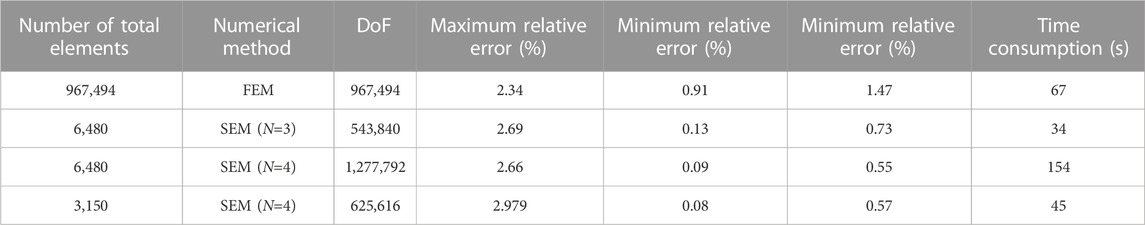
TABLE 1. Statistics of mesh discretization and time consumption for the different numerical methods.

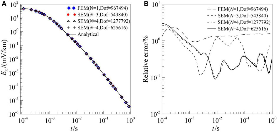
FIGURE 3

FIGURE 3. $E_x$ responses and relative error corresponding to the model shown in Figure 2, $E_x$ responses of the FEM and SEM (A), and the relative errors compared to the 1D semi-analytical solution (B).

As for the analysis in terms of efficiency, based on the comparisons of the time consumptions of the different methods in Table 1, the sorting order for the numerical methods from minimum to maximum computational time is as follows: third-order SEM with a detailed mesh, fourth-order SEM with a coarse mesh, unstructured tetrahedral FEM, and fourth-order SEM with a detailed mesh. Among them, the modeling of third-order SEM with a detailed mesh has the shortest computational time, the fewest degrees of freedom, and the lowest accuracy. The modeling of the fourth-order SEM with a detailed mesh has the longest computational time, maximum degrees of freedom, and the highest accuracy. It is worth noting that the fourth-order SEM with a coarse mesh, under the condition of fewer degrees of freedom, exhibits better computational efficiency and accuracy compared to the conventional FEM. In addition, the fourth-order SEM with coarse detailed meshes has the same accuracy level, which means that in situations with high-accuracy modeling, increasing the grid density may not contribute significantly to improving the accuracy but significantly affect computational efficiency. Therefore, in some cases, further increasing the mesh density may not significantly enhance the accuracy of the results but rather increase the computational complexity and cost.

It is important to strike a balance between the accuracy requirements, computational efficiency, and associated costs. By comparing with conventional FEM, SEM can provide higher accuracy results while maintaining a relatively lower computational cost. For FEM, it uses the first-order vector basis function for the interpolation and requires that a refined mesh subdivision be generated to guarantee the modeling accuracy, which leads to a sharp increase in the degrees of freedom (DoF) and affects the modeling efficiency. Therefore, SEM can offer a good balance between accuracy and computational efficiency, making it a suitable choice for various applications. Because the high-order GLL basis function with spectral convergence is used in SEM, which only slightly depends on the mesh subdivision, it can obtain more accurate modeling results. In summary, using SEM for the forward modeling of 3D TEM has a higher accuracy and efficiency.

For long-wire source TEM response, the accuracy of SEM is also further studied. First, we set a 3D model with a high resistance background and a conductive anomalous cuboid embedded (Figure 4), and we compared the results of SEM with those of the unstructured tetrahedral FEM. The detailed parameters were as follows: the conductive cuboid size is 200 m × 400 m × 400 m, and the top surface is 400 m; the resistivities of the anomaly and background were $E_x$ and $E_x$, respectively; and the coordinates of the center of the anomalous body were (0 m, 1,000 m, 600 m). We set a long-wire source extending 100 m in the x-direction. The center coordinate is (0 m, 0 m, 0 m), and the transmitting current intensity is 100 A. The survey points were laid out within a 600 m × 800 m area located directly above the anomalous body, with a survey point spacing of 25 m and 825 survey points. We applied the same waveform as the three-layer model used. To further investigate the modeling capability of SEM, the third-order SEM was applied, and an element scale of 50 m × 50 m × 50 m was used to discretize the target modeling area. The total number of discrete elements was 8,360, and the DoF were 699,672. DoF for the FEM were 1,141,968.

FIGURE 4

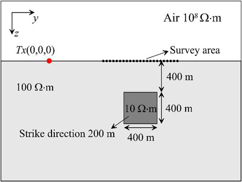
FIGURE 4. Schematic diagram of the yz-profile of the 3D earth model (the length of the source).

Figure 5 shows the $E_x$ contour distribution for different time channels for SEM and FEM. Figures 5A–E present the FEM results, and Figures 5F–J present the SEM results. Figure 6 shows a comparison of the $E_x$ responses at the survey point of (0 m, 1,000 m, 0 m) for FEM and SEM. As can be seen from Figures 5, 6, the results of the two methods are consistent, and the difference of the relative errors is under 3.00%. These results indicate that SEM is efficient and applicable to 3D long-wire source TEM forward modeling.

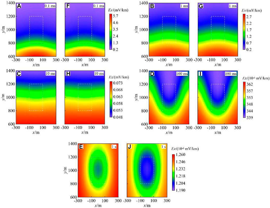
FIGURE 5

FIGURE 5. $E_x$ contour distribution for different time channels for SEM and FEM. (A–E) Results for FEM and (F–J) results for SEM.

FIGURE 6

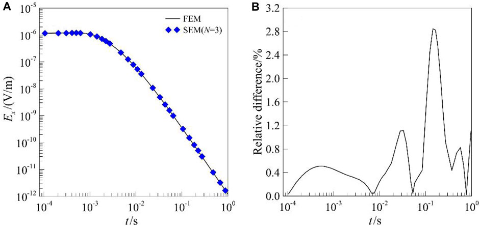
FIGURE 6. $E_x$ responses and relative difference of SEM and FEM for the survey point of (0 m, 1,000 m, 0 m). E_x response (A), B is relative errors (B).

To investigate the characteristics of the underground current density distribution, we calculated the underground current density of the 3D model in Figure 4 for the channels of [0, 1, 3, 5] ms. The modeling area is $\left(x,y,z\right)\in \left[-1000\mathrm{m},1000\mathrm{m}\right]\times 1000\mathrm{m}\times \left[0\mathrm{m},2000\mathrm{m}\right]$. Figure 7 shows the current density distribution. It can be seen that the underground material produces an eddy current field, which is opposite to the direction of the current density for the on-time interval, and decays and propagates downward over time.

FIGURE 7

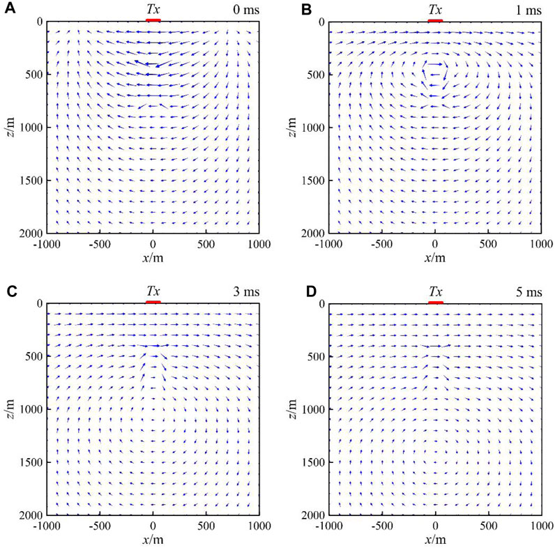
FIGURE 7. Distribution of the current density in the y=1,000 m profile for different time channels. The blue arrow indicates the direction and magnitude of the underground current density. Current density at time channel 0 ms (A), current density at time channel 1 ms (B), current density at time channel 3 ms (C), current density at time channel 5 ms (D).

Geoelectric model for shale gas reservoir fracturing monitoring

Hydraulic fracturing technology is a core technique used in the development of unconventional oil and gas resources, as well as enhanced geothermal systems. Its purpose is to modify the reservoir by creating effective artificial fracture zones and maintaining sustainable production. The dynamic monitoring of the reservoir physical property changes during the hydraulic fracturing process is a key technology for predicting and evaluating the volume modification of the fracturing treatment. It plays a significant role in optimizing fracturing operations and increasing production while reducing costs. After the injection of fracturing fluid into the reservoir, a low-resistivity anomaly is formed, which exhibits significant electrical contrast with the surrounding rocks. Therefore, EM methods have unique advantages over microseismic-based methods in identifying fluid characteristics. With the improvement of instrument equipment and data acquisition techniques, EM monitoring technology has been continuously maturing and has become a research hotspot for unconventional reservoir monitoring. In recent years, since the high-power long-wire TEM method, which has the outstanding advantage of deep detection at a low cost, researchers have been paying much attention to applying this in the field of hydraulic fracturing monitoring. However, the target area of hydraulic fracturing is mainly composed of fractured media with a large burial depth and small scale, so developing a method of extracting the effective signal (the variations in the TEM response between the pre-fracturing and post-fracturing) caused by the hydraulic fracturing is a key step in TEM. Yan et al. (2018) carried out continuous TEM investigations of monitoring shale hydraulic fracturing in the Jiaoshiba National Shale Gas Development Zone and successfully captured the EM signal changes caused by fracturing of the target layer at a depth of 3 km. In addition, Hoversten et al. (2015); Hoversten and Schwarzbach (2021) proved that the long-wire TEM has the capability of detection with a 3 km depth using the 3D forward modeling tests, which further indicates the detection validity of TEM for the hydraulic fracturing reservoirs.

To explore the feasibility of using long-wire source TEM for monitoring hydraulic fracturing in a practical region, we designed a practical shale gas reservoir model (Figure 8) with a scale of 300 m × 1,000 m × 300 m based on the well-logging and petrophysical information for the Jiaoshiba National Shale Gas Development Zone in China. The geoelectrical resistivity model based on JIAOYE 1# well-logs is shown in Table 2 (referred to Yan et al., 2018). According to the resistivity model of JIAOYE 1#, the practical geoelectric model is set up in Figure 8. The length of each fracturing stage was 500 m along the y-direction, and the resistivity of the formation before and after fracturing were separately 50 Ω·m and 5 Ω·m, respectively. We calculated the variations in the TEM responses for two fracturing stages. Referring to Yan et al. (2018), the long-wire transmitting source with the current intensity of 100 A extends 5000 m along the x-direction. The coordinate of the central point was (0 m, 0 m, 0 m). The survey points with a spacing of 100 m were laid out over [−500 m, 500 m] × [3,500 m, 6,500 m]. The waveform of the transmitting current we applied was a bipolar square with a 4-s period. We used an 80 m × 80 m × 80 m element scale to discretize the target modeling area and adopted the third-order SEM to calculate the TEM responses.

FIGURE 8

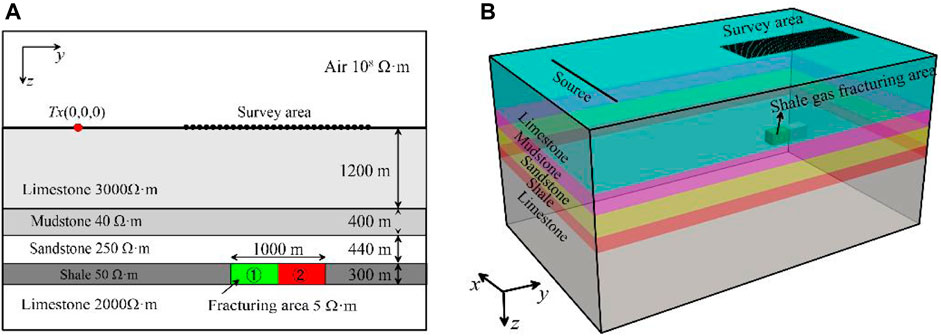
FIGURE 8. 3D earth model for the shale gas reservoir fracturing monitoring. 2D yz cross-section (A), 3D model diagram (B).

TABLE 2

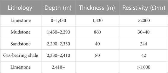
TABLE 2. Geoelectrical resistivity model based on Jiaoye 1# well logs.

Figure 9 shows the residual voltage variations of a single surveying point (0 m, 5,000 m, 0 m) at different time channels during the two fracturing stages. Figure 10 shows the residual voltage contour surface between the pre-fracturing and post-fracturing periods for time channels of 1 ms, 10 ms, and 100 ms. It can be seen from Figure 10 that 1) based on the residual voltage contour surface, the fracturing range in the xy-plane differs for the different time channels, and a reverse voltage occurs at 100 ms. Compared with the residual voltage at the three time channels, the fracturing area delineated by the residual voltage at 10 ms is more accurate. This may be because the EM signals decay with depth and time, so the detection depth of the EM signals at 1 ms is less than the depth of the fracturing formation, while that at 100 ms is too large to exceed the fracturing target layer. 2) Regarding the voltage differences of the two fracturing stages, as the number of fracturing stages increases, the voltage differences increase significantly. For the instrument, limited by resolution and signal-to-noise ratio, the voltage differences of less than 10 $\mu V$ cannot be distinguished by the sensor. Based on our modeling results, our method can capture the EM signal changes caused by two-stage fracturing. Therefore, the distribution of the shale gas fracturing can be easily delineated with high-power and long-wire source TEM, even when the fracturing area has a large burial depth and small scale. This demonstrates that the long-wire source TEM has a good prospect for use in shale gas fracturing monitoring.

FIGURE 9

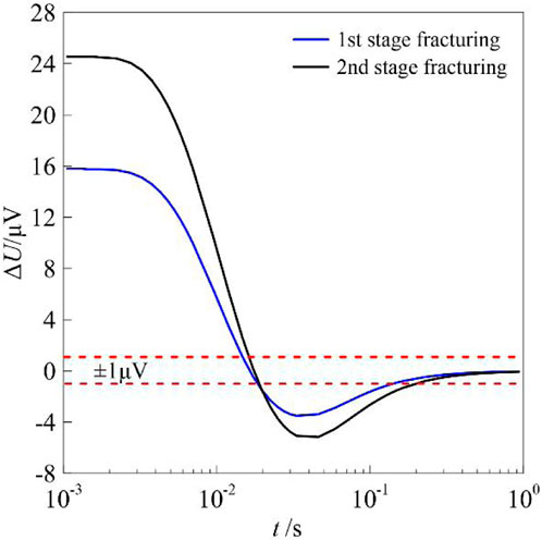
FIGURE 9. Residual voltage between the pre-fracturing and post-fracturing periods at the survey point of (0 m, 5,000 m, 0 m).

FIGURE 10

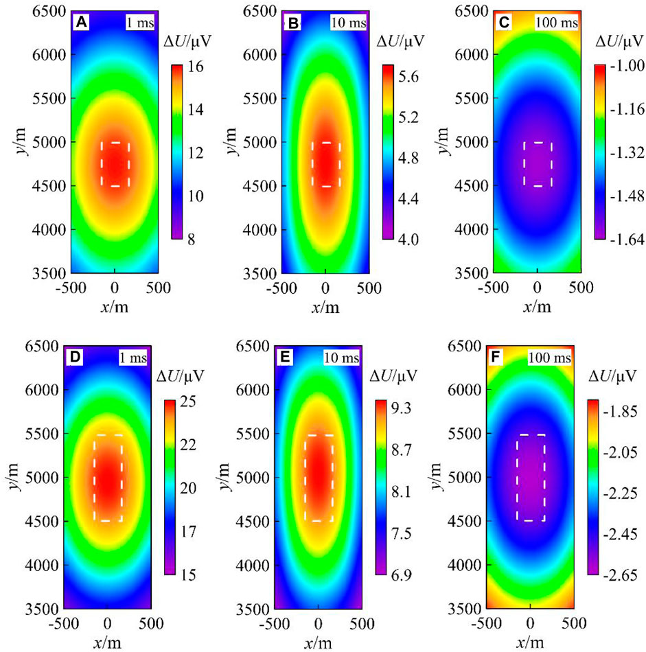
FIGURE 10. Residual voltage contour surface between the pre-fracturing and post-fracturing periods. (A–C) Residual voltage in the first stage and (D–F) residual voltage in the second stage; the areas denoted by the dotted line are the fracturing range in the xy-plane.

To further explore the variation mechanism of the physical field between pre-fracturing and post-fracturing, the characteristics of current density are analyzed and shown in Figure 11. As shown, the EM wave propagates in the lossy medium, and $E_x$ and current density decay continuously. Moreover, it produced a significant current channel effect in the shale low-resistance layer of the fracturing area. Based on the normal continuity of current density, the amplitudes of $E_x$ for the shale layer are significantly smaller than those of the surrounding medium. It is worth noting that with the passage of time, the distribution of $E_x$ and current density in Figure 11 occurred in the reverse amplitude. With the analysis in Figure 7, in the early time channel, the eddy current center is mainly concentrated in the shallow underground layer, the fracturing area is at the lower part of the eddy current center, and the current density points to the negative direction of x-axis; with the eddy current propagating, the fracturing area changes to the upper part of the eddy current center, and the direction of the current density points to x-axis. Thus, the distribution of $E_x$ and current density are reversed. Thus, the distribution characteristics of current density show that the process of hydraulic fracturing can lead to EM field variation, which is the essential reason why the long-wire source TEM method can monitor shale gas fracturing.

FIGURE 11

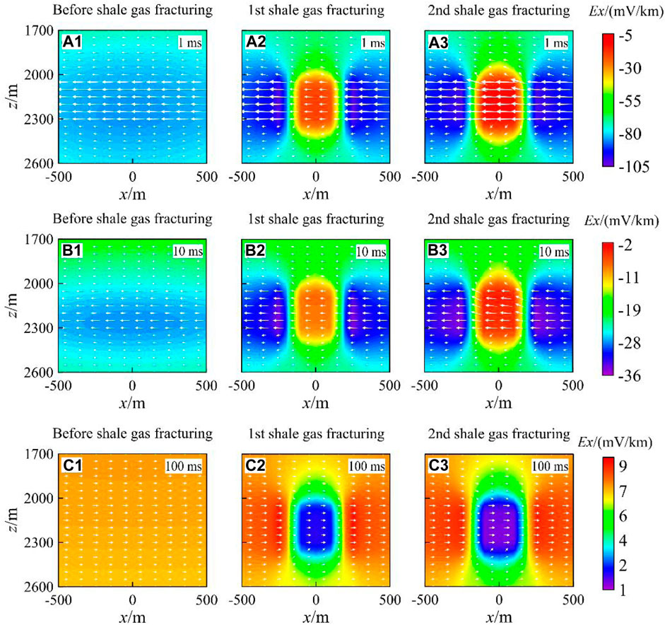
FIGURE 11. Distributions of $E_x$ and the current density in profile y = 5,000 for different time channels; the white arrow indicates the direction and magnitude of the underground current density. Before shale gas fracturing at time channel 1 ms (A1), after 1st shale gas fracturing at time channel 1 ms (A2), after 2nd shale gas fracturing at time channel 1 ms (A3), before shale gas fracturing at time channel 10 ms (B1), after 1st shale gas fracturing at time channel 10 ms (B2), after 2nd shale gas fracturing at time channel 10 ms (B3), before shale gas fracturing at time channel 1 ms (C1), after 1st shale gas fracturing at time channel 100 ms (C2), after 2nd shale gas fracturing at time channel 100 ms (C3).

Therefore, by calculating the TEM response of a relatively simple model for electrical resistivity with isotropy, we can confirm that by analyzing the changes in EM signals collected during multiple segmented fracturing processes, it is possible to identify anomalies in the target zone of the fracturing fluid. However, when a large amount of water or fracturing fluid is injected into reservoir layers, the fluid flows along microfractures and continuously expands the fractures. This process may lead to an increase in the porosity and permeability of the reservoir and causes anisotropy (Kirkby et al., 2016). Therefore, it is essential to study the characteristics of TEM responses in anisotropic media during fracturing monitoring processes. In the future, we will focus on the TEM response forward modeling of anisotropic electrical models.

Conclusion

We successfully introduced SEM into 3D long-wire source TEM forward modeling. With the comparison of the SEM, FEM and 1D semi-analytical solution on 1D and 3D models, the high accuracy and efficiency of SEM are verified. In addition, the impact of mesh subdivision and the basis function order on accuracy and efficiency are analyzed. It is proved that the modeling accuracy can be improved by mesh refinement and increasing basis function order. In addition, we applied SEM to modeling the TEM response in the application of shale gas fracturing monitoring, and confirmed that we can capture the EM signal variation caused by the conductivity change of the thin-bed reservoir. Via analyzing the current density of yz-profiles for pre-fracturing, first post-fracturing, and second post-fracturing, we further confirmed that the long-wire source TEM method can be used for fracturing monitoring.

In future research, we will continue to optimize SEM algorithms and use deformed meshes to adapt to more complex electrical models. We will also introduce parallel computing techniques to further improve the computational efficiency. In addition, we will delve into the application of TEM forward modeling with SEM in hydraulic fracturing monitoring. By incorporating rock physics information and considering more realistic geological conditions, we will introduce anisotropic electrical models and explore the characteristics of segmented TEM responses in the presence of electrical anisotropy for hydraulic pressure monitoring, which can lay the foundation for the development of techniques for identifying and extracting anisotropic signals in the target area of hydraulic fracturing, and serve as a theoretical basis for the analysis of measured TEM data in the hydraulic fracturing monitoring area.

Data availability statement

The raw data supporting the conclusion of this article will be made available by the authors, without undue reservation.

Author contributions

XH: methodology and writing–original draft. LY: conceptualization, funding acquisition, supervision, and writing–review and editing. XW: data curation, formal analysis, methodology, validation, visualization, and writing–original draft. XX: conceptualization, project administration, validation, visualization, and writing–review and editing. LZ: funding acquisition, investigation, methodology, and writing–original draft. XC: formal analysis, funding acquisition, and writing–review and editing.

Funding

The authors declare financial support was received for the research, authorship, and/or publication of this article. This paper is financially supported by the China Natural Science Foundation (42030805, 42104070, 42274103, and 42374096), the Natural Science Foundation Project of Hubei Province (2022CFB229), the Key Laboratory of Geophysical Electromagnetic Probing Technologies of the Ministry of Natural Resources (KLGEPT202204), and the Open Fund of Key Laboratory of Exploration Technologies for Oil and Gas Resources (Yangtze University), Ministry of Education (PI2023-02).

Conflict of interest

The authors declare that the research was conducted in the absence of any commercial or financial relationships that could be construed as a potential conflict of interest.

Publisher’s note

All claims expressed in this article are solely those of the authors and do not necessarily represent those of their affiliated organizations, or those of the publisher, the editors, and the reviewers. Any product that may be evaluated in this article, or claim that may be made by its manufacturer, is not guaranteed or endorsed by the publisher.

References

Abdallah, S., Utsugi, M., Aizawa, K., Uyeshima, M., Kanda, W., Koyama, T., et al. (2020). Three-dimensional electrical resistivity structure of the Kuju volcanic group, Central Kyushu, Japan revealed by magnetotelluric survey data. J. Volcanol. Geotherm. Res. 400, 106898. doi:10.1016/j.jvolgeores.2020.106898

CrossRef Full Text | Google Scholar

Ahmadian, M., LaBrecque, D., Liu, Q. H., Slack, W., Brigham, R., Fang, Y., et al. (2018). “Demonstration of proof of concept of electromagnetic methods for high resolution illumination of induced fracture networks” in SPE Hydraulic Fracturing Technology Conference and Exhibition. Society of Petroleum Engineers.

Google Scholar

Bhuyian, A. H., Landrø, M., and Johansen, S. E. (2012). 3D CSEM modeling and time-lapse sensitivity analysis for subsurface CO2 storage. Geophysics 77 (5), 343–E355. doi:10.1190/geo2011-0452.1

CrossRef Full Text | Google Scholar

Boaga, J., Renzi, S., Vignoli, G., Deiana, R., and Cassiani, G. (2012). From surface wave inversion to seismic site response prediction: beyond the 1D approach. Soil Dyn. Earthq. Eng. 36, 38–51. doi:10.1016/j.soildyn.2012.01.001

CrossRef Full Text | Google Scholar

Ceia, M. A. R., Carrasquilla, A. A. G., Sato, H. K., and Lima, O. (2007). Long offset transient electromagnetic (LOTEM) for monitoring fluid injection in petroleum reservoirs - preliminar results of fazenda alvorada field (Brazil). Seg. Glob. Meet. Abstr., 60–64. doi:10.1190/sbgf2007-013

CrossRef Full Text | Google Scholar

Cohen, G. (2003). Higher-order numerical methods for transient wave equations. Phys. Today 56 (3), 70–71. doi:10.1063/1.1570776

CrossRef Full Text | Google Scholar

Commer, M., Hoversten, G. M., and Um, E. S. (2015). Transient-electromagnetic finite–difference time–domain earth modeling over steel infrastructure. Geophysics 80 (2), E147–E162. doi:10.1190/geo2014-0324.1

CrossRef Full Text | Google Scholar

Commer, M., and Newman, G. (2004). A parallel finite–difference approach for 3D transient electromagnetic modeling with galvanic sources. Geophysics 69 (5), 1192–1202. doi:10.1190/1.1801936

CrossRef Full Text | Google Scholar

Cox, L. H., Wilson, G. A., and Zhdanov, M. S. (2012). 3D inversion of airborne electromagnetic data. Geophysics 77 (4), WB59–WB69. doi:10.1190/geo2011-0370.1

CrossRef Full Text | Google Scholar

Di, Q., Zhu, R., Xue, G., Yin, C., and Li, X. (2019). New development of the Electromagnetic (EM) methods for deep exploration. Chin. J. Geophys. (in Chinese) 62 (6), 2128–2138. doi:10.6038/cjg2019M0633

CrossRef Full Text | Google Scholar

Didana, Y. L., Heinson, G., Thiel, S., and Krieger, L. (2017). Magnetotelluric monitoring of permeability enhancement at enhanced geothermal system project. Geothermics 66, 23–38. doi:10.1016/j.geothermics.2016.11.005

CrossRef Full Text | Google Scholar

Gharti, H. N., Langer, L., and Tromp, J. (2019). Spectral-infinite-element simulations of coseismic and post-earthquake deformation. Geophysical Journal International 216 (2), 1364–1393. doi:10.1093/gji/ggy495

CrossRef Full Text | Google Scholar

Hördt, A., Druskin, V. L., Knizhnerman, L. A., and Strack, K. (1992). Interpretation of 3-D effects in long-offset transient electromagnetic (LOTEM) soundings in the Münsterland area/Germany. Geophysics 57 (9), 1127–1137. doi:10.1190/1.1443327

CrossRef Full Text | Google Scholar

Hoversten, G. M., Commer, M., Haber, E., and Schwarzbach, C. (2015). Hydro-frac monitoring using ground time-domain electromagnetics. Geophysical Prospecting 63 (6), 1508–1526. doi:10.1111/1365-2478.12300

CrossRef Full Text | Google Scholar

Hoversten, G. M., and Schwarzbach, C. (2021). Monitoring hydraulic fracture volume using borehole to surface electromagnetic and conductive proppant. Geophysics 86 (1), E93–E109. doi:10.1190/geo2020-0410.1

CrossRef Full Text | Google Scholar

Huang, X., Yin, C., Cao, X., Liu, Y. H., Zhang, B., and Cai, J. (2017). 3D anisotropic modeling and identification for airborne EM systems based on the spectral-element method. Applied geophysics 14 (3), 419–430. doi:10.1007/s11770-017-0632-y

CrossRef Full Text | Google Scholar

Huang, X., Yin, C., Farquharson, C. G., Cao, X., Zhang, B., Huang, W., et al. (2019). Spectral-element method with arbitrary hexahedron meshes for time-domain 3D airborne electromagnetic forward modeling. Geophysics 84 (1), E37–E46. doi:10.1190/geo2018-0231.1

CrossRef Full Text | Google Scholar

Khan, S., Shafique, M., Vander, M., and Van der Werff, H. (2020). Scenario-based seismic hazard analysis using spectral element method in northeastern Pakistan. Natural hazards 103 (2), 2131–2144. doi:10.1007/s11069-020-04074-w

CrossRef Full Text | Google Scholar

Kirkby, A., Heinson, G., and Krieger, L. (2016). Relating permeability and electrical resistivity in fractures using random resistor network models. Journal of Geophysical Research Solid Earth 121 (3), 1546–1564. doi:10.1002/2015jb012541

CrossRef Full Text | Google Scholar

Komatitsch, D., Vilotte, J. P., Vai, R., Castillo-Covarrubias, J. M., and Sánchez-Sesma, F. J. (1999). The spectral element method for elastic wave equations-application to 2-D and 3-D seismic problems. International Journal for numerical methods in engineering 45 (9), 1139–1164. doi:10.1002/(sici)1097-0207(19990730)45:9<1139::aid-nme617>3.0.co;2-t

CrossRef Full Text | Google Scholar

Lee, J. H., and Liu, Q. H. (2004). “Analysis of 3D eigenvalue problems based on a spectral element method” in Int. Union Radio Science (URSI) Meeting Abstract. Monterey, CA, 30.

Google Scholar

Lee, J. H., Xiao, T., and Liu, Q. H. (2006). A 3-D spectral-element method using mixed-order curl conforming vector basis functions for electromagnetic fields. IEEE transactions on Microwave Theory and Techniques 54 (1), 437–444. doi:10.1109/tmtt.2005.860502

CrossRef Full Text | Google Scholar

Li, J., Hu, X., Cai, H., and Liu, Y. (2020). A finite-element time-domain forward–modelling algorithm for transient electromagnetics excited by grounded-wire sources. Geophysical Prospecting 68 (4), 1379–1398. doi:10.1111/1365-2478.12917

CrossRef Full Text | Google Scholar

Liu, R., Liu, J., Wang, J., Liu, Z., and Guo, R. (2020). A time-lapse CSEM monitoring study for hydraulic fracturing in shale gas reservoir. Marine and Petroleum Geology 120, 104545. doi:10.1016/j.marpetgeo.2020.104545

CrossRef Full Text | Google Scholar

Liu, Y., Teng, J., Lan, H., Si, X., and Ma, X. (2014). A comparative study of finite element and spectral element methods in seismic wavefield modeling. Geophysics 79 (2), T91–T104. doi:10.1190/geo2013-0018.1

CrossRef Full Text | Google Scholar

Liu, Y., Yogeshwar, P., Hu, X., Peng, R., Tezkan, B., Mörbe, W., et al. (2020). Effects of electrical anisotropy on long-offset transient electromagnetic data. Geophysical Journal International 222 (2), 1074–1089. doi:10.1093/gji/ggaa213

CrossRef Full Text | Google Scholar

Lu, G., and Li, Y. (2007). The study of spectral element method in electromagnetic fields: international symposium on antennas. IEEE.

Google Scholar

Lu, X., Farquharson, C. G., Miehé, J. M., and Harrison, G. (2021). 3D electromagnetic modeling of graphitic faults in the Athabasca Basin using a finite-volume time-domain approach with unstructured grids. Geophysics 86 (6), B349–B367. doi:10.1190/geo2020-0657.1

CrossRef Full Text | Google Scholar

Mulder, W. A., Wirianto, M., and Slob, E. C. (2008). Time-domain modeling of electromagnetic diffusion with a frequency-domain code. Geophysics 73 (1), F1–F8. doi:10.1190/1.2799093

CrossRef Full Text | Google Scholar

Orange, A., Key, K., and Constable, S. (2009). The feasibility of reservoir monitoring using time-lapse marine CSEM. Geophysics 74 (2), F21–F29. doi:10.1190/1.3059600

CrossRef Full Text | Google Scholar

Patera, A. T. (1984). A spectral element method for fluid dynamics: laminar flow in a channel expansion. Journal of computational Physics 54 (3), 468–488. doi:10.1016/0021-9991(84)90128-1

CrossRef Full Text | Google Scholar

Peacock, J. R., Thiel, S., Heinson, G. S., and Reid, P. (2013). Time-lapse magnetotelluric monitoring of an enhanced geothermal system. Geophysics 78 (3), B121–B130. doi:10.1190/geo2012-0275.1

CrossRef Full Text | Google Scholar

Peacock, J. R., Thiel, S., Reid, P., and Heinson, G. (2012). Magnetotelluric monitoring of a fluid injection: example from an enhanced geothermal system. Geophys Res Lett 39 (17), 3–7. doi:10.1029/2012gl053080

CrossRef Full Text | Google Scholar

Rønquist, E. M., and Patera, A. T. (1987). A Legendre spectral element method for the Stefan problem. International journal for numerical methods in engineering 24 (12), 2273–2299. doi:10.1002/nme.1620241204

CrossRef Full Text | Google Scholar

Sasaki, Y., Yi, M. J., Choi, J., and Son, J. S. (2015). Frequency and time domain three-dimensional inversion of electromagnetic data for a grounded-wire source. Journal of Applied Geophysics 112, 106–114. doi:10.1016/j.jappgeo.2014.09.016

CrossRef Full Text | Google Scholar

Schamper, C., Rejiba, F., Tabbagh, A., and Spitz, S. (2011). Theoretical analysis of long offset time-lapse frequency-domain controlled source electromagnetic signals using the method of moments: application to the monitoring of a land oil reservoir. Journal of Geophysical Research Solid Earth 116 (B3), B03101. doi:10.1029/2009jb007114

CrossRef Full Text | Google Scholar

Strack, K. (2010). Advances in electromagnetics for reservoir monitoring. GEOHORIZONS 2010 (6), 1–4.

Google Scholar

Strack, K. (2014). Future directions of electromagnetic methods for hydrocarbon applications. Surv. Geophys. 35 (1), 157–177. doi:10.1007/s10712-013-9237-z

CrossRef Full Text | Google Scholar

Streich, R. (2016). Controlled-source electromagnetic approaches for hydrocarbon exploration and monitoring on land. Surveys in geophysics 37 (1), 47–80. doi:10.1007/s10712-015-9336-0

CrossRef Full Text | Google Scholar

Tietze, K., Ritter, O., Patzer, C., Veeken, P., and Dillen, M. (2019). Repeatability of land-based controlled-source electromagnetic measurements in industrialized areas and including vertical electric fields. Geophysical Journal International 218 (3), 1552–1571. doi:10.1093/gji/ggz225

CrossRef Full Text | Google Scholar

Tietze, K., Ritter, O., and Veeken, P. (2015). Controlled-source electromagnetic monitoring of reservoir oil-saturation using a novel borehole-to-surface configuration. Geophys. Prospect. 63 (6), 1468–1490. doi:10.1111/1365-2478.12322

CrossRef Full Text | Google Scholar

Um, E. S., Harris, J. M., and Alumbaugh, D. L. (2010). 3D time-domain simulation of electromagnetic diffusion phenomena: a finite-element electric-field approach. Geophysics 75 (4), F115–F126. doi:10.1190/1.3473694

CrossRef Full Text | Google Scholar

Wang, L., Yin, C., Liu, Y., Yang, S., Xiu-Yan, R., Zhe-Jian, H., et al. (2021). Three-dimensional forward modeling for the SBTEM method using an unstructured finite-element method. Applied Geophysics 18 (1), 101–116. doi:10.1007/s11770-021-0863-9

CrossRef Full Text | Google Scholar

Yan, L., Chen, X., Tang, H., Xie, X. B., Zhou, L., Hu, W. B., et al. (2018). Continuous TDEM for monitoring shale hydraulic fracturing. Applied Geophysics 15 (1), 26–34. doi:10.1007/s11770-018-0661-1

CrossRef Full Text | Google Scholar

Zhdanov, M. S., Endo, M., Black, N., Spangler, L., Fairweather, S., Gibbs, A., et al. (2013). Electromagnetic monitoring of CO2 sequestration in deep reservoirs. First Break 31, 85–92. doi:10.3997/1365-2397.31.2.66662

CrossRef Full Text | Google Scholar

Zhou, Y., Shi, L., Liu, N., Zhu, C., and Liu, Q. H. (2016). Spectral element method and domain decomposition for low-frequency subsurface EM simulation. IEEE Geoscience and Remote Sensing Letters 13 (4), 550–554. doi:10.1109/lgrs.2016.2524558

CrossRef Full Text | Google Scholar

Zhou, Y., Shi, L., Liu, N., Zhu, C., Sun, Y., and Liu, Q. H. (2017). Mixed spectral-element method for overcoming the low-frequency breakdown problem in subsurface EM exploration. IEEE Transactions on Geoscience and Remote Sensing 55 (6), 3488–3500. doi:10.1109/tgrs.2017.2674685

CrossRef Full Text | Google Scholar

Zhu, J., Yin, C. C., Liu, Y. S., Liu, Y. H., Liu, L., Yang, Z. L., Qiu, C. K., et al. (2020). 3-D dc resistivity modelling based on spectral element method with unstructured tetrahedral grids. Geophysical Journal International 220 (3), 1748–1761. doi:10.1093/gji/ggz534

CrossRef Full Text | Google Scholar