Software techniques for training restricted Boltzmann machines on size-constrained quantum annealing hardware

Restricted Boltzmann machines are common machine learning models that can utilize quantum annealing devices in their training processes as quantum samplers. While this approach has shown promise as an alternative to classical sampling methods, the limitations of quantum annealing hardware, such as the number of qubits and the lack of connectivity between the qubits, still pose a barrier to wide-scale adoption. We propose the use of multiple software techniques such as dropout method, passive labeling, and parallelization techniques for addressing these hardware limitations. The study found that using these techniques along with quantum sampling showed comparable results to its classical counterparts in certain contexts, while in others the increased complexity of the sampling process hindered the performance of the trained models. This means that further research into the behavior of quantum sampling needs to be done to apply quantum annealing to training tasks of more complicated RBM models.

1. Introduction

When training a well-known machine learning model called restricted Boltzmann machine (RBM), the gradient estimation process for the weights and biases requires the taking samples from a probability distribution called the Boltzmann distribution. While there are classical methods for this process, such as the Contrastive Divergence (CD) algorithm, they are known to grow computationally expensive as the model grows in size (Adachi and Henderson, 2015). An interesting alternative for this classical sampling process is generating these samples using quantum computation devices called quantum annealers (Hauke et al., 2020). While most of the contemporary use cases for these devices are focused on finding low-energy states for quantum systems, these devices have shown promise for sampling data points from the Boltzmann distribution of Hamiltonian energy functions (Adachi and Henderson, 2015; Dixit et al., 2021). This feature of quantum annealing devices has wide applicability in training of classical machine learning models, such as RBM (Restricted Boltzmann Machine) or layer-wise pretraining of more complicated deep learning algorithms. While these models are not on par with the leading industry-level machine learning models, they provide a task where it is quite simple to compare the performance of these quantum techniques with classical techniques, which are of high academic interest.

Quantum sampling have some advantages, such as being faster on large layer sizes or showing improved performance on learning tasks, over the conventional sampling algorithms, such as Gibbs sampling or the contrastive divergence algorithm (Hinton, 2002). These algorithms, especially Gibbs sampling, are relatively slow and do not produce accurate estimations of the underlying probability distribution (Carreira-Perpiñán and Hinton, 2005). While these algorithms have been deemed good enough for classical use cases, it is still vital to compare them with novel quantum sampling-based approaches to determine whether the switch from classical to quantum can be deemed practical.

The quantum sampling approach does have its own set of issues as follows: (1) The accuracy of the technique is highly dependent on device parameters related to the annealing process, and no known way of determining these parameters exists properly yet; (2) it is not known whether the technique can even produce proper samples from the Boltzmann distribution; and (3) size limitations imposed on the machine learning model by the hardware itself cause the problem space to be limited to toy examples, instead of actually useful real-world problems.

This article will focus mostly on the last issue and proposes and evaluates several techniques to circumvent some obstacles caused by hardware limitations. First of these is the use of extreme rates of unit dropout to reduce the effective layer width of RBMs during the sampling process. The second technique is to use passive labeling schemes to reduce the total width of the visible layer, by disabling all labeling units during the training and adding their influence to the hidden layer as a modifier to the bias of the hidden unit during sampling. Finally, the article will take a look into the inherent parallelism of the quantum annealing device and provide insight into how this technique can have wide use cases on quantum sampling. It is important to note that this last technique does not allow training our models in smaller hardware, but it shows ways that RBMs could take advantage of hypothetical future hardware, especially in tandem with the unit dropout method.

The study shows that while classical methods require fewer epochs for well-behaving models, the end result after a longer period of training can be closely the same, or sometimes even better, which is in line with previous research. The unit dropout method further accentuates this effect and, in our experiments, performs demonstrably worse compared with classical dropout techniques. The reasons for this are analyzed in the Section 7 of the article. The parallelization schemes seem to somewhat lower the performance of the training but decrease the time-to-solution of each round of estimating the model distribution drastically. Finally, the passive labeling strategy shows promise for evaluating the performance of quantum sampling, without any hardware-related costs.

The key contributions of this article are as follows:

• Proposing these techniques for alleviating the presented hardware-related issues and evaluating the effects and the limitations to use a theoretical setting (Section 4).

• Developing an experimental setup to evaluate how these techniques perform when training RBMs against classical methods in similar contexts and showing their benefits and restrictions (Sections 5, 6).

• Providing discussion on the results and how current generation quantum annealing hardware needs to scale to be usable in these sampling tasks (Section 7).

2. Related research

Restricted Boltzmann machine has been studied extensively for a very long time (Hinton and Sejnowski, 1983), but their usefulness has become more apparent in the last decade (Hinton, 2012). Research on classical sampling methods gained traction when the Contrastive Divergence algorithm was discovered, which allowed RBMs to be trained more efficiently compared with the older sampling methods (Carreira-Perpiñán and Hinton, 2005). The dropout algorithm featured in this article has been researched quite extensively, showing improvements on performance and also working as a weight regularization method for many different machine learning models (Srivastava et al., 2014).

The use of quantum annealing in sampling tasks has been researched widely, and it has shown some advantages over classical sampling methods, despite the stated issues. In the study by Adachi and Henderson (2015), quantum annealing was used to pretrain a deep belief network, which showed increased performance over classical sampling methods on a Bars and Stripes dataset. In the study by Dixit et al. (2021) quantum annealing was shown to be as effective as classical sampling methods when training the RBM on a cybersecurity ISCX dataset. Pelofske et al. (2022) presented the technique for parallelizing QUBO problems for quantum annealing devices, which is particularly useful for training RBMs as presented in this study.

There is also a study conducted on a purely quantum version of the more general Boltzmann Machines that are called QBMs (Quantum Boltzmann Machines) (Amin et al., 2018). There are also Quantum Born Machines, which have shown quite a bit of promise in various generative machine learning tasks, that share a lot of their underlying math with Boltzmann Machines (Coyle et al., 2020). It is important to note that these quantum machine learning models are most often implemented in gate-based quantum hardware, as opposed to quantum annealing hardware.

3. Theoretical background

Restricted Boltzmann Machines are simple neural networks that can be applied to various machine learning tasks (Hinton, 2012). In practice, they are mostly used in the pretraining phase of more complex machine learning models such as deep belief networks (Hinton et al., 2006). They are characterized by a visible and a hidden layer of units connected bilaterally, and the units are activated using the sigmoid function.

These models are based on the Ising model: a mathematical representation of ferromagnetic system, where the stochastic behavior of the system is governed by a Hamiltonian energy function E. With this function, the probability P, often also referred to as the Boltzmann distribution, of a system being in a certain configuration can be computed using the following equations:

$\begin{array}{ll}\begin{array}{lll}E(v,h)\hfill & =\hfill & -\underset{i}{{{\displaystyle \sum }}^{\text{}}}{b}_i{h}_i-\underset{i}{{{\displaystyle \sum }}^{\text{}}}{c}_i{v}_i-\underset{i,j}{{{\displaystyle \sum }}^{\text{}}}{w}_{i,j}{v}_i{h}_j\hfill \end{array}& (1)\end{array}$

$\begin{array}{llll}P(v,h)& =& Z^{-1}{e}^{E(v,h)/T}& (2)\end{array}$

where σ is the collection of units in an RBM with possible states {0, 1}. b_i and c_i are the bias values of the hidden and visible units h_i and v_i. w_{i, j} is the weight of the connection between units v_i and h_j. Z is the partition function over all possible combinations of σ that normalizes the probability to be between 0 and 1. T is the temperature of the system, which is often normalized as 1. The structure of a RBM is visualized in the Figure 1.

FIGURE 1

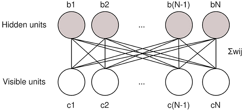
Figure 1. Restricted Boltzmann machines have a hidden and a visible layer of units with biases b_i and c_i, connected by weights w_ij.

Training these models requires finding a set of parameters θ, which makes the model distribution P mimic an unknown data distribution Q that characterizes the problem. These parameters can be found by minimizing the Kullback-Leibler divergence between these two distributions, which, in turn, can be approximated by minimizing the average negative log-likelihood of the model distribution (Joyce, 2011; Hinton, 2012). This ultimately results in the following training rules for weights and biases which can be used for gradient descent:

$\begin{array}{llll}\partial w_{ij}\hfill & =\hfill & \eta \left({\langle v_i{h}_j\rangle }_{data}-{\langle v_i{h}_j\rangle }_{model}\right)\hfill & (3)\end{array}$

$\begin{array}{llll}\partial b_i\hfill & =\hfill & \eta \left({\langle h_i\rangle }_{data}-{\langle h_i\rangle }_{model}\right)\hfill & (4)\end{array}$

$\begin{array}{llll}\partial c_i\hfill & =\hfill & \eta \left({\langle v_i\rangle }_{data}-{\langle v_i\rangle }_{model}\right)\hfill & (5)\end{array}$

where η is the learning rate and < ..>_data and < ..>_model, respectively, are the data and model distributions of the system.

The important thing to notice here is the fact that estimating the data distribution of an RBM can be done easily using classical algorithms, but estimating the model distribution is considered to be analytically intractable. This is due to the partition function, which requires the algorithm to compute the total energy of the system for all possible configurations of σ. This requires O(2ⁿ) computations where n is the number of units in the system, which means that alternative methods for estimating this distribution are needed.

Instead of computing an exact solution for the model distribution, sampling methods are used to get an estimate of the model distribution. If it is possible to draw accurate samples from the probability distribution P, the average of these samples can form a proper estimate of the model distribution. This is usually done using the Contrastive Divergence (CD) algorithm, where the states of the visible and hidden layers are inferred repeatedly from each other, starting from the initial data vector v assigned to the visible units (Carreira-Perpiñán and Hinton, 2005). The number of cycles in this process can influence the accuracy of the resulting model depending on the problem at hand. Even one iteration has been found to converge toward the correct solution, more iterations can result in improved accuracy of the resulting model (Carreira-Perpiñán and Hinton, 2005). Increasing the number of cycles is a very expensive process, which is why more efficient sampling methods can provide more benefits in tasks that require training RBMs. Contrastive divergence is often marked by appending the number of cycles after the CD abbreviation, i.e., contrastive divergence with one cycle becomes CD-1.

3.1. Sampling from the Boltzmann distribution using quantum annealing

Quantum annealing is a novel alternative to universal quantum computing, where, instead of using gate operations to modify the states of the qubits in the device, it implements a physical system that corresponds to the Ising Model (Hauke et al., 2020). Mathematically, the quantum annealing process implements a Hamiltonian function as follows:

$\begin{array}{llll}H(\tau )& =& A(\tau )H_D+B(\tau )H_P& (6)\end{array}$

$\begin{array}{ll}{H}_D=-{\displaystyle \sum _{i\in V}{\sigma }_i^x}& (7)\end{array}$

$\begin{array}{ll}{H}_P={\displaystyle \sum _{ij\in ℰ}{J}_{ij}}{\sigma }_i^z{\sigma }_j^z+{\displaystyle \sum _{i\in V}{h}_i}{\sigma }_i^z& (8)\end{array}$

where H_D is the initial Hamiltonian of the system, and H_P is the target Hamiltonian which describes the problem at hand. ${\sigma }_i^x$ and ${\sigma }_i^z$ are Pauli matrices localized to qubit i, A(τ) and B(τ) are time-dependent monotonic functions, which describe the schedule in which H_D is transformed into H_P, when normalized annealing time τ moves from 0 to 1. J_{i, j} and h_i are the parameters that describe the interactions between the qubits of the system.

Quantum annealing devices are capable of finding ground states for Hamiltonian systems, due to the adiabatic theory of quantum mechanics. While this has been contested before, after years of research, it has become quite evident that these devices can be also used to sample from the Boltzmann distribution of the given Hamiltonian (Benedetti et al., 2016). This could benefit the process of training RBMs drastically, as the model distribution of an RBM can be approximated by an average of samples taken from the Boltzmann distribution of the model.

Sampling from the Boltzmann distribution of the model requires small changes to the quantum annealing process. The control parameters of the system have to be scaled down by a parameter called the effective temperature B_eff, which allows the system to thermalize more freely during the annealing (Benedetti et al., 2016). Choosing the correct value for this parameter can be difficult, as it seems to be dependent on multiple factors, like the size of the system and the parameters of the system itself. This choice is often done before the training process by evaluating the performance of the parameter against classical methods on similarly sized models and keeping it constant during the training process.

There is also research suggesting that only using B_eff to scale the parameters of the model can be insufficient while using alternative annealing schedules provided by current generation quantum annealing devices can help to alleviate these issues (Marshall et al., 2019). For example, pausing the annealing in the middle of the process can improve the accuracy sampling process, provided that the pause happens on a correct region, which is again dependent on the model parameters. The process of reverse annealing has also shown promise for improving the sampling accuracy.

While the sampling capabilities of quantum annealing devices are promising, the limited device sizes and the constraint they impose on the layer sizes of RBMs are still the key limiting factors on applying quantum annealing to machine learning problems (Dumoulin et al., 2013). As the connectivity between qubits is very limited in the current generation quantum annealing devices, embedding fully connected RBMs requires chaining qubits together. This imposes a maximum layer width on the trained RBMs, which is still far away from conventionally used layer sizes, which can have easily over 1,000 units in a single layer. The quantum annealing device DWave 2000Q has a theoretical maximum layer width of 64 units, and while DWave Advantage does not yet have a known theoretical maximum layer width, the modern embedding heuristics are capable of finding embeddings with a layer width of 128 units.

4. Materials and methods

This section describes various methods which can be used to circumvent limitations that arise due to maximum layer sizes imposed by the small qubit counts and the effects of limited topology of current generation quantum annealing hardware.

4.1. The unit dropout method

Unit Dropout is a widely adopted weight regularization method for neural networks, originally developed for RBMs (Srivastava et al., 2014). In this method, during training, units from the model are dropped out with probability p, usually referred to as the dropout rate. It is also possible to keep the amount of dropped-out units constant, in which case we can describe the dropout process using a variable called S_max, which is the amount of units kept in the RBM Layer. This process is presented in Figure 2. The training will, then, resume for the pruned network for the duration of a single batch, and the parameter updates will be computed for the pruned network. After this, the units that were dropped out are returned to normal, and the process can repeat until the training has been completed. This has been shown to regularize the weights very efficiently and to be resilient against overfitting during training (Srivastava et al., 2014).

FIGURE 2

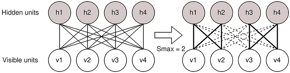
Figure 2. Example of the dropout process. Here, the total layer width is 4 units and before sampling half of the units are dropped out from the model. The remaining weights are shown using bolded lines between the units.

This method is very convenient for the purpose of training Restricted Boltzmann Machines using quantum annealing, as it automatically prunes the model to a smaller subset of the original one. This means that the new model will be easier to fit inside a contemporary quantum annealing device. The dropout rate can also be tweaked to control the size of the model that will be embedded into the quantum annealing device, allowing for a lot of control over the resulting model.

When using this method in tandem with quantum annealing, small modifications need to be made to the original algorithm to take into account the limits imposed by the quantum annealing device. Instead of using a probabilistic dropout rate p, constant S_max number of units should be picked from the model with uniform probability. In this way, it is easier to ensure that the model can still be embedded into the device, and it also allows us to reuse the same embedding scheme for the duration of the training, which is useful as computing an embedding scheme for a problem is an expensive process (Cai et al., 2014). If S_max/N_units ≤ 0.5, multiple subsets of size S_max can be chosen from the units of the model, making the training more efficient, as these models can be sampled in parallel. Existing research places the optimal value for the dropout rate approximately 0.5, but this rate can be pushed further to allow larger layer sizes to be trained using existing quantum annealing devices, as shown in Section 5.

4.2. Passive labeling

While RBMs are often used for unsupervised learning tasks, they are also capable of supervised learning by adding predictive label units to the hidden layer of the network. Because these additional units can be treated as additional visible units in the system, it is often convenient to use different activation functions, like the softmax activation function, for them, as this can improve the predictive capabilities of the network. Though this works quite well for classical sampling algorithms, the core assumption of quantum annealing assumes the likelihood of a unit coming from the Boltzmann distribution. This means that alternative activation functions are not viable for quantum-sampled RBMs.

Adding labeling units into the RBM is useful, as they provide a clear metric for the fitness of the training process, as opposed to measuring the reconstruction error of the model or evaluating the generative capabilities of the model by eye. For quantum sampled RBMs, this can be difficult, as adding labels to the system takes valuable space in the embedding map, increases total chain length of the system, and breaks the symmetry of the total area required by the model. We have developed a novel technique of adding labels to RMBs called the passive labeling technique to address these inconveniencies.

In passive labeling, an average influence of the label units on the hidden units is computed classically before the sampling starts using any activation function. This influence can, then, be added to the bias of the hidden unit for the duration of the sampling procedure, while all the labeling units are kept out from the sampling process.

$\begin{array}{ll}{h}_i^{passive}=h_i+\text{softmax}({\displaystyle \sum _{k\in l}{l}_k}{w}_{i,k}^{label})& (9)\end{array}$

where l is the set of labeling units, and $w_{i,k}^{label}$ is the weight associated with the hidden unit h_i and labeling unit l_k.

After the states of the units are sampled, the states of the labeling units can be inferred from the hidden states classically, and these states can be used to compute the parameter gradients of the label units. This should cause only a slight cost for the accuracy of the learning process, with no requirements imposed on the sampling compared with the unsupervised learning methods. If the purpose of the labeling is to evaluate the effectiveness of the sampling techniques for the quantum annealing algorithms, this cost should be more than reasonable, compared with the apparent cost of adding multiple label units to the system.

4.3. Inherent parallelism of quantum annealing

Whenever quantum annealing is used for sampling from systems, it is possible that many of the qubits that are not connected to the embedded model are left unused during the sampling. This is especially wasteful when the problem size is much smaller than the maximum allowed. As shown in the study mentioned in the reference (Pelofske et al., 2022), smaller problems can be embedded into quantum annealing device multiple times, as shown in Figure 3, which reduces the time-to-solution of the problem greatly. This technique is especially interesting for quantum sampling, as using novel annealing control techniques, such as mid-annealing pauses, can increase the overall sampling time by a large margin. This means that the overhead of embedding the problem multiple times into the annealing device will become quite negligible, as the time of taking each sample can increase from the default value of 20μs to even 1, 000μs.

FIGURE 3

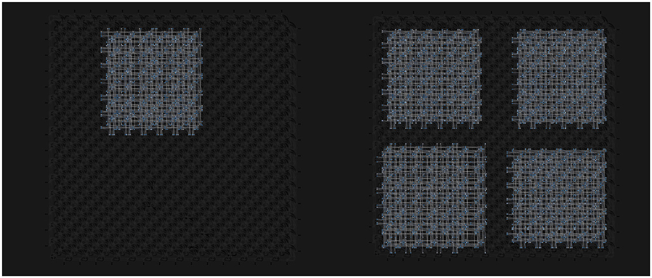
Figure 3. Example of problem parallelization on quantum annealing devices: On the left, a single 64 × 64 RBM is embedded into the device, leaving many of the qubits unused during sampling. On the right, the 64 × 64 RBM has been embedded into the device four times, allowing these RBMs to be sampled simultaneously. These RBMs can be identical or distinct from one another depending on the use case. An image is created using DWave visualization tools.

There are two main ways in which this parallelism technique can help in the process of quantum sampling. The first one is reducing the number of samples to 1/N of the original size, where N is the number of times in which the problem will fit into the sampling device (Pelofske et al., 2022). The other way is an intersection between using the dropout technique and the inherent parallelism of the quantum annealing device, taking the pruned networks from the dropout process, embedding them all into the quantum annealing device, and producing samples for them in parallel. This method of parallelism should outperform the original one in relation to time, as the time-consuming calls to the quantum sampling device will be reduced to the 1/N of the original amount, negating a lot of unnecessary networking overhead while also increasing the amount of work that can be now done in parallel by the classical processes.

While this technique does not address the issue of limited hardware, a reasonable assumption is that if these techniques become viable in future, the growth of the possible hardware will allow us to further take advantage of the computational resources we have. Even on current generation hardware, this technique managed to save a lot of computational resources and time, as shown in the Section 6 of the article.

5. Experimental setup

The techniques presented were evaluated by training restricted Boltzmann machines on a custom-made generated bars and stripes dataset, which is presented in Figure 4. This allowed for strict control over the overall size N_problem of the dataset and the difficulty of the machine learning task itself, as a variable amount of noise was introduced to the dataset to make the task more difficult. Using these rules, a labeled training set of 10,000 images, a prediction set of 2,000 images, and an evaluation set of 2,000 images were created. The training dataset is, then, divided into 20 batches for training, and the relatively large batch size was chosen to save computational resources. Two distinct datasets were created for evaluating the different qualities of the algorithm: the 64-pixel dataset and the 256-pixel dataset.

FIGURE 4

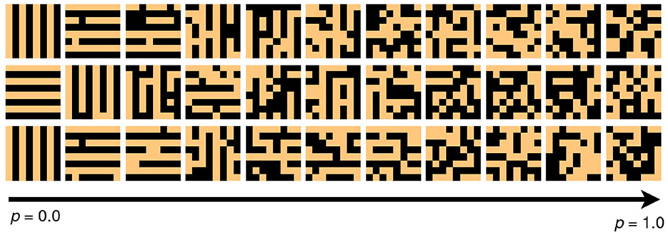
Figure 4. Examples 8x8 images generated for testing the learning methods of this study from noise level p = 0.0 to p = 1.0. The dataset is divided into images of bars (vertical stripes) and stripes (horizontal stripes), after which noise is introduced to the image by randomizing each pixel with the probability of p. The choice of this probability p determines how difficult this learning task will be. These images for the study were created with p = 0.7.

The 64-pixel bars and stripes problem was formulated for testing out how embedding one RBM multiple times into the quantum annealing device compares to embedding it a single time performance-wise. This dataset allowed us to also test how parallel embedding of RBMs affects the performance of the training algorithm.

The 256-pixel bars and stripes problem was formulated for looking into the effects of drastic rates of dropout used in tandem with quantum annealing. Multiple RBMs were trained with various rates of unit dropout, using the CD-1 sampling and quantum annealing. The effects of embedding multiple RBMs into the device and sampling them at the same time were also tested.

The RBM implementation was written in python, and the quantum sampling was implemented using the APIs of the DWave Leap platform and AWS platform. The quantum sampling implementation targeted the DWave Advantage quantum annealing device, for which the embedding schemes were precomputed using the DWave MinorMiner tool (Cai et al., 2014). The parameters of the annealing procedure were chosen manually by evaluating the L1 distance between the gradients of the quantum sampling approach and classical Gibbs sampling with 1,000 cycles. Additional evaluation of techniques was done by classical means.

An effective temperature of 1.0 was chosen for annealing by evaluating the accuracy of the gradient estimation for different values. A pause of 10μs was introduced in the middle of the annealing process, which improved the sampling accuracy by a sizeable margin. Five spin reversal transforms were used to ensure that the device-specific errors would not affect the learning process that much. Each gradient update was computed from 100 samples taken from the annealer. Finally, the strength of the chain between logically coupled qubits was set to 1, which was essential for achieving well-trained models during the training.

Classical machine learning parameters were chosen by training various models classically and picking the best one for quantum sampling approaches. This was hardly the ideal method for choosing parameters, as there is no guarantee that the ideal classical parameters for the quantum sampling method mirror the classical methods, but as training the models using quantum annealing was very time-consuming and expensive, this way was chosen due to convenience.

The experimental setup was affected by the fact that while the process of sampling from the quantum annealer itself is very fast, the API calls to the cloud platforms for each of the quantum annealing tasks were very slow, as most of the time was spent on queues waiting to get access to the annealing device.

6. Results

Figure 5 shows results for training multiple RBMs using different sampling approaches. As can be seen, quantum sampling performs similarly or worse than classical sampling approaches. It has to be noted that this performance could be improved with more careful choices for the annealing parameters.

FIGURE 5

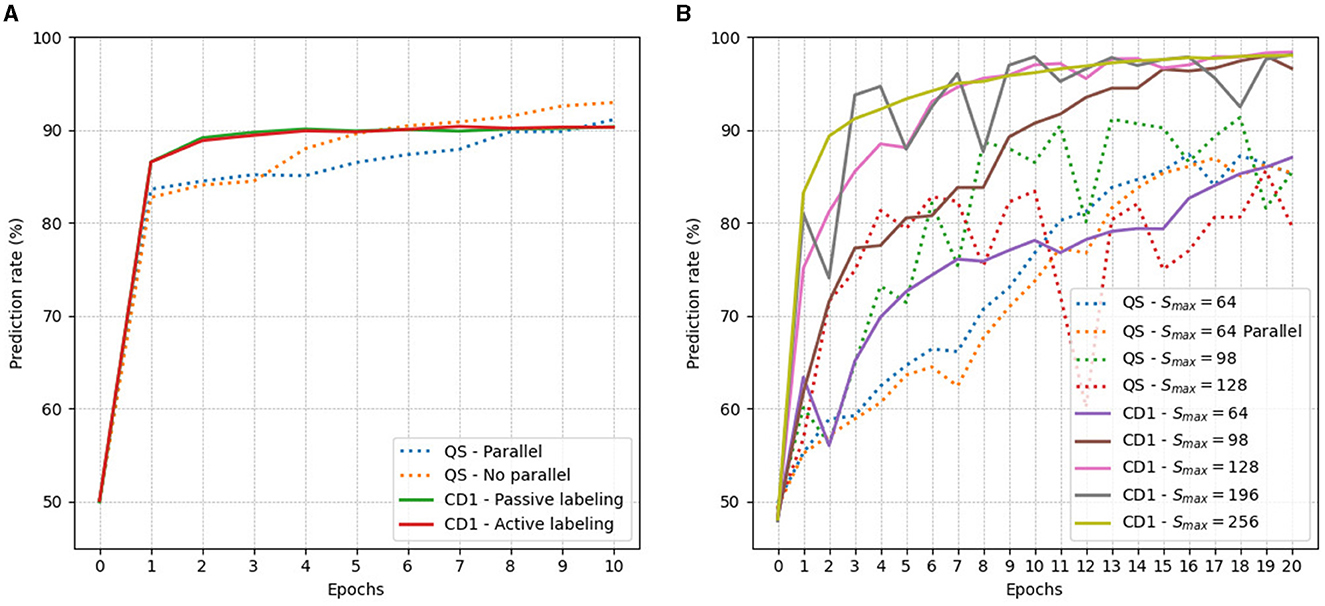
Figure 5. Prediction rates of RBMs that have been trained for 20 epochs. QS indicates quantum sampling and CD-1 contrastive divergence with one sampling step (A) results of 8 × 8 Bars and Stripes problem trained on RBM with 64 visible and hidden units. (B) Results of 16 × 16 Bars and Stripes problem trained on RBM with 256 visible and hidden units with various rates of dropout.

In the 64-pixel dataset, quantum annealing managed to achieve higher prediction rates compared to the classical approach, but the training process required more epochs. This result is in line with previous findings on the performance of the quantum annealing in these sampling tasks (Adachi and Henderson, 2015; Benedetti et al., 2016; Dixit et al., 2021). Initially, the parallel and non-parallel sampling approaches were in line with one another, but in the end, the non-parallel approach outperformed the parallel one. In the classical training case, the passive labeling scheme was completely identical compared to the traditional sampling approach, but in other more complex problems, it showed consistent slight decreases in accuracy. Parallelizing sampling reduced the time that it took to generate the samples from around 98 ms to 84 ms, which is not a huge decrease, but this gap could widen, if advanced annealing control schemes would be used during the annealing.

In the 256-pixel dataset, the classical sampling methods outperformed the quantum ones quite consistently. Only one of the classical sampling methods with the largest rate of the dropout was in line with the quantum sampling approach. The results of these quantum-sampled RBMs also were a lot noisier compared to classical RBMs. The effects of dropout on the prediction rates were quite consistent with existing research for about halfway into the training (Srivastava et al., 2014), as the lower dropout rates seemed to outperform the higher ones until the quantum sampling approaches seemed to converge into the same region of prediction rates. The parallel and non-parallel quantum sampling approaches were again very similar to the 64-pixel dataset until the difference converged in the end. Here the real difference is in the time-to-solution of the parallel and non-parallel sampling methods, which is quite drastic. Taking 100 samples for four different RBMs at the same time would take about 110 ms, compared to about 390 ms when taken subsequently. This does not take into account the overhead from networking-related tasks with the communication with the classical computer and quantum platforms, which could take anywhere from a couple of seconds to a couple of minutes of real-time when conducting this study, further widening the gap between the parallel and non-parallel sampling methods.

7. Discussion

Quantum sampling seems to perform similarly to classical sampling methods in the 64-pixel bars and stripes problem. While classical sampling methods find the well-performing model parameters faster, quantum sampling seems to catch up with the classical methods after some additional training. The prediction rates of quantum sampled RBMs seem to be sometimes more unstable during training, probably due to the noisiness of the gradient estimation. These results indicate that quantum sampling can at least be considered to be a good alternative for estimating the model distribution of a Hamiltonian energy function, to the contemporary classical method of CD-1.

The largest issue with using the quantum sampling approach comes from the larger parameter space, which needs to be controlled for the duration of the training (Benedetti et al., 2016). Device parameters need to be chosen well enough for the training to be effective and there are no known heuristics for choosing them correctly, other than applying some commonly used default values for them. The optimal values for these parameters can be dependent on the embedded problem, which makes constantly evaluating new values for them during the training an intractable task. Finding a heuristic for estimating these parameters could be vital for the commercial viability of the quantum sampling approach.

The passive labeling strategy seemed to perform well in this learning task when comparing the prediction rates for conventional classical training methods and using the passive labeling scheme classically, though its performance can suffer when using it on more complicated machine learning tasks. This means that this method of attaching labels without any increase to the effective size of the embedded problem can be used to evaluate the performance of quantum sampling methods. As most often RBMs are used only for pretraining more complicated deep neural networks like deep belief networks (Hinton et al., 2006), attaching labels this way is probably not needed in industry-level machine learning tasks. It provides a more concrete way of looking into the effectiveness of quantum sampling, compared to reconstruction rate or evaluating generated sampled images out of the network.

The dropout method, when used in tandem with quantum sampling, seems to produce more volatile results as shown in Figure 5B. As both techniques introduce some noise in the gradient estimation process, the resulting quantum sampled models ended up performing worse than their classical counterparts. This could be because of poor parameter choices for many of the quantum annealed RBMs, as the only model that behaved similarly to the classical equivalent was the S_max = 64 model, which was also incidentally the model size which was used for determining the hyperparameters for the training. It is also possible that the use of the dropout technique is not compatible with these quantum sampling techniques. Further research on the topic of unit dropout and quantum annealing should be done, but this was not possible to do here due to a lack of access to quantum hardware. The key takeaway is that better heuristics for device parameters could allow introducing dropout into quantum sampling in actual use cases.

Parallelizing quantum sampling tasks into the quantum annealing device showed a slight decrease in performance but lowered the time-to-solution of the problem by a good margin. This is especially true when using these parallelization techniques in tandem with the dropout technique, allowing us to sample from all the sub-RBMs at the same time. Likely, the upper limit of the number of different RBMs that could be embedded into the quantum annealing device is two, as the optimal value for the dropout rate dictates that going beyond 0.5 will only hinder the training process. This can still give us results about two times faster than normal, and these two distinct sub-RBMs can be further parallelized, assuming that the device size itself is large enough.

Quantum annealing devices have already grown quite large from the point of view of qubit counts, and further advances in hardware will bring us new ways quantum computing can be used to benefit existing computational methods. The importance of this study can be seen at two points in time in relation to hardware advancements: (1) in the near term these techniques can be used to train up to two or three times wider networks than normally would be possible due to hardware limitations and (2) in long term these techniques allow for parallelizing the training process of pruned networks, reducing the number of API calls or samples needed for completing quantum sampling tasks. Both of these possibilities are dependent on whether exploring the rather large hyperparameter space of quantum sampled RBMs becomes convenient in the future.

8. Conclusion

While the current generation quantum annealing devices are still quite small in the context of using them for quantum sampling, the industry leader of quantum annealing devices DWave has already envisioned creating larger devices with more advanced connectivity schemes (DWave, 2021). But despite the rapid development of hardware, it is still important to try to bridge the gap between it and the software side, as reaching applicability as early as possible can be vital for adoption on larger scales. It also has to be noted that whether quantum annealing can provide a proper quantum advantage in computational problems is still a highly debated topic (Hauke et al., 2020).

The unit dropout method can be seen as a convenient way of pruning RBM layers into more palatable chunks for next-generation quantum annealing devices, while the parallelization techniques can be used to compute these chunks in parallel on the same annealing device, saving precious computational time, especially on the classical side of things. The passive labeling scheme instead should be thought of as a convenient way of adding labels to RBMs without having to think about their effect on the embedding of the RBM into the hardware itself.

Some possible pitfalls of adopting quantum sampling as a method of evaluating the model distribution function of a Hamiltonian is the increased parameter space caused by the device parameters related to the annealing process. Quite a lot of work shows that choosing the effective temperature of the model can be an intractable task, which is why a lot of research ends up choosing a fiat default value for the duration of the training. Also moving away from the API model of quantum computing to a more integrated model, where the classical computer and the quantum computer work closely together will be vital for any of these speed-ups to matter.

Data availability statement

The original contributions presented in the study are publicly available. This data can be found at: GitHub, https://github.com/Ilmosal/QDBN.

Author contributions

IS: Conceptualization, Formal analysis, Investigation, Methodology, Software, Validation, Visualization, Writing—original draft, review, and editing. JN: Funding acquisition, Supervision, Writing—review and editing.

Funding

The author(s) declare financial support was received for the research, authorship, and/or publication of this article. This work was partly funded by Business Finland Quantum Computing Campaign project FrameQ (8578/31/2022) and ITEA3 programme project IVVES (ITEA-2019-18022-377).

Acknowledgments

The authors would like to express gratitude to Valter Uotila from the University of Helsinki for providing access to computational resources for the AWS platforms' quantum devices.

Conflict of interest

The authors declare that the research was conducted in the absence of any commercial or financial relationships that could be construed as a potential conflict of interest.

Publisher's note

All claims expressed in this article are solely those of the authors and do not necessarily represent those of their affiliated organizations, or those of the publisher, the editors and the reviewers. Any product that may be evaluated in this article, or claim that may be made by its manufacturer, is not guaranteed or endorsed by the publisher.

References

Adachi, S., and Henderson, M. (2015). Application of quantum annealing to training of deep neural networks. arXiv preprint arXiv:1510.06356. doi: 10.48550/arXiv.1510.06356

CrossRef Full Text | Google Scholar

Amin, M. H., Andriyash, E., Rolfe, J., Kulchytskyy, B., and Melko, R. (2018). Quantum Boltzmann machine. Phys. Rev. X 8, 021050. doi: 10.1103/PhysRevX.8.021050

CrossRef Full Text | Google Scholar

Benedetti, M., Realpe-Gomez, J., Biswas, R., and Perdomo-Ortiz, A. (2016). Estimation of effective temperatures in quantum annealers for sampling applications: a case study with possible applications in deep learning. Phys. Rev. A 94. doi: 10.1103/PhysRevA.94.022308

CrossRef Full Text | Google Scholar

Cai, J., Macready, W., and Roy, A. (2014). A practical heuristic for finding graph minors. arXiv preprint arXiv:1406.2741. doi: 10.48550/arXiv.1406.2741

CrossRef Full Text | Google Scholar

Carreira-Perpiñán, M. Á., and Hinton, G. E. (2005). “On contrastive divergence learning,” in International Conference on Artificial Intelligence and Statistics.

Google Scholar

Coyle, B., Mills, D., Danos, V., and Kashefi, E. (2020). The born supremacy: quantum advantage and training of an ising born machine. NPJ Quant. Inform. 6, 60. doi: 10.1038/s41534-020-00288-9

CrossRef Full Text | Google Scholar

Dixit, V., Selvarajan, R., Aldwairi, T., Koshka, Y., Novotny, M., Humble, T., et al. (2021). Training a quantum annealing based restricted Boltzmann machine on cybersecurity data. IEEE Trans. Emerg. Top. Comput. Intell. 6, 417–428.

Google Scholar

Dumoulin, V., Goodfellow, I. J., Courville, A., and Bengio, Y. (2013). On the challenges of physical implementations of RBMs. arXiv preprint arXiv:1312.5258. doi: 10.1609/aaai.v28i1.8924

CrossRef Full Text | Google Scholar

DWave (2021). Zephyr Topology of D-Wave Quantum Processors.

Google Scholar

Hauke, P., Katzgraber, H. G., Lechner, W., Nishimori, H., and Oliver, W. D. (2020). Perspectives of quantum annealing: methods and implementations. Rep. Prog. Phys. 83, 054401. doi: 10.1088/1361-6633/ab85b8

PubMed Abstract | CrossRef Full Text | Google Scholar

Hinton, G., Osindero, S., and Teh, Y.-W. (2006). A fast learning algorithm for deep belief nets. Neural Comput. 18, 1527–1554. doi: 10.1162/neco.2006.18.7.1527

PubMed Abstract | CrossRef Full Text | Google Scholar

Hinton, G., and Sejnowski, T. (1983). “Optimal perceptual inference,” in Proceedings of the IEEE conference on Computer Vision and Pattern Recognition (Washington, DC), 448–453.

Google Scholar

Hinton, G. E. (2002). Training products of experts by minimizing contrastive divergence. Neural Comput. 14, 1771–1800. doi: 10.1162/089976602760128018

PubMed Abstract | CrossRef Full Text | Google Scholar

Hinton, G. E. (2012). “A practical guide to training restricted Boltzmann machines,” in Neural Networks: Tricks of the Trade, eds G. Montavon, K.-R. Müller, and G. B. Orr (Berlin; Heidelberg: Springer), 599–619.

Google Scholar

Joyce, J. (2011). Kullback-Leibler Divergence. Berlin; Heidelberg: Springer.

Google Scholar

Marshall, J., Venturelli, D., Hen, I., and Rieffel, E. G. (2019). Power of pausing: advancing understanding of thermalization in experimental quantum annealers. Phys. Rev. Appl. 11, 044083. doi: 10.1103/PhysRevApplied.11.044083

CrossRef Full Text | Google Scholar

Pelofske, E., Hahn, G., and Djidjev, H. N. (2022). Parallel quantum annealing. Sci. Rep. 12, 4499. doi: 10.1038/s41598-022-08394-8

CrossRef Full Text | Google Scholar

Srivastava, N., Hinton, G., Krizhevsky, A., Sutskever, I., and Salakhutdinov, R. (2014). Dropout: a simple way to prevent neural networks from overfitting. J. Mach. Learn. Res. 15, 1929–1958.

Google Scholar