Benefit of vertical localization for sea surface temperature assimilation in isopycnal coordinate model

Sea surface temperature (SST) observations are a critical data set for long-term climate reconstruction. However, their assimilation with an ensemble-based data assimilation method can degrade performance in the ocean interior due to spurious covariances. Assimilation in isopycnal coordinates can delay the degradation, but it remains problematic for long reanalysis. We introduce vertical localization for SST assimilation in the isopycnal coordinate. The tapering functions are formulated empirically from a large pre-industrial ensemble. We propose three schemes: 1) a step function with a small localization radius that updates layers from the surface down to the first layer for which insignificant correlation with SST is found, 2) a step function with a large localization radius that updates layers down to the last layer for which significant correlation with SST is found, and 3) a flattop smooth tapering function. These tapering functions vary spatially and with the calendar month and are applied to isopycnal temperature and salinity. The impact of vertical localization on reanalysis performance is tested in identical twin experiments within the Norwegian Climate Prediction Model (NorCPM) with SST assimilation over the period 1980–2010. The SST assimilation without vertical localization greatly enhances performance in the whole water column but introduces a weak degradation at intermediate depths (e.g., 2,000–4,000 m). Vertical localization greatly reduces the degradation and improves the overall accuracy of the reanalysis, in particular in the North Pacific and the North Atlantic. A weak degradation remains in some regions below 2,000 m in the Southern Ocean. Among the three schemes, scheme 2) outperforms schemes 1) and 3) for temperature and salinity.

1. Introduction

Climate reanalyzes are dynamically consistent reconstructions of the climate system. They are highly in demand by the climate research community and serve for understanding anthropologically driven global warming and its impact, mechanisms of climate variability and teleconnections, and are used for initializing climate predictions. Atmospheric reanalyzes (e.g., ERA-Interim, Dee et al., 2011) and oceanic reanalyzes (e.g., ORAS5, Zuo et al., 2019) have been produced for a while and can achieve a high degree of accuracy. Coupled reanalyzes (e.g., Brune et al., 2015; Counillon et al., 2016; Laloyaux et al., 2018a; O'Kane et al., 2021) have emerged as they better account for coupled dynamics of the climate, and help to better understand coupled variability mechanisms. Such initiative is also well suited to initialize the climate prediction model with a coupled reanalysis from the same model, as it limits physical inconsistencies in initial conditions between different components (i.e., initial shocks Balmaseda and Anderson, 2009; Mulholland et al., 2015).

Nowadays coupled reanalyzes are getting extended for the full instrumental period (i.e., from 1850). Sea surface temperature (SST) observation is the primary source of instrumental oceanic measurements prior to 1950. The raw SST measurements are very cumbersome to use because they combine very various types of measurements (e.g., methods of bucket retrieval, thermometer and satellite remote sensing) and thus have different representativity, uncertainty and bias. It is a common practice in climate research to use SST analysis products that derive a coordinated estimate from pre-calibrated measurements. The Hadley Centre Sea Ice and Sea Surface Temperature (HadISST, Rayner et al., 2003) is one of such products and covers the period 1850–present. It provides an estimate of SST and its uncertainty and is a critical dataset for climate reanalyzes (Counillon et al., 2016; Laloyaux et al., 2018a). Its stochastic property (i.e., 10 realizations) is critical to optimally account for SST uncertainty for long-term reanalysis.

Data assimilation (DA, Kalnay et al., 1996; Carrassi et al., 2018) is a statistical method that can estimate the optimal model state based on observations, the dynamical model and their statistical information. Ensemble DA methods (e.g., the ensemble Kalman filter (EnKF), Evensen, 2003) make use of an ensemble of model simulations (e.g., multiple realizations of an Earth system model) to estimate the forecast error covariances and propagate information from the observed variables into the non-observed variables (i.e., multivariate updates). Such a method also allows the forecast error covariances to evolve with the variability of the climate system (i.e., flow-dependent), which is important to handle climate regime shifts (Zhang et al., 2007; Karspeck et al., 2013; Brune et al., 2015; Counillon et al., 2016).

A practical limitation of using the ensemble DA method in a high-dimensional system is that one can only afford a limited number of realizations [${O}$(10), a limited ensemble size], much smaller than the degree of freedom of the system (Miyoshi et al., 2014). The forecast error covariances estimated by the relatively small ensemble suffer spurious covariances that are caused by sampling error and cause a degradation of the assimilation particular at long distances. To limit the impact of these sample noises in the forecast error covariances, one has to rely on an auxiliary regularization technique known as localization (Hamill et al., 2001; Houtekamer and Mitchell, 2001). Localization either filters the forecast error covariances by multiplying element by element (Schur product) with a distance-dependent function (e.g., Houtekamer and Mitchell, 2001) that decreases from 1 (at the observation location) to 0 at some radial distances, or tapers observation error variance with the reciprocal of the distance-dependent function in a local framework (e.g., Evensen, 2003). The two schemes are comparable (Sakov and Bertino, 2010). Localization is well suited to geophysical applications in which typical covariances decay as a function of the distance. An excessive localization (e.g., a too-short localization radius) will under-use observations, while insufficient localization (e.g., a too-large localization radius) will let spurious variability introduce artificial signals. Tapering is used to ensure continuity in the update, but it may as well distort the covariance (Miyoshi et al., 2014). Localization function is often isotropic, but Ménétrier et al. (2015a) explicitly formulated heterogeneous/anisotropic localization function through the optimal linear filtering theory and the centered moment estimation theory. Such a localization function has been applied in numerical weather prediction systems (Ménétrier et al., 2015b; Laloyaux et al., 2018b). Localization in the isopycnal coordinate ocean model has been mostly applied horizontally, but less commonly applied in the vertical. It is because assimilation in isopycnal limits spurious covariance and propagates updates at the deep ocean by formulating the covariance in a dynamical manner (e.g., Counillon and Bertino, 2009).

Isopycnal coordinate ocean models are a specific type of ocean models that are vertically discretised with potential densities (Bleck et al., 1992). They allow for excellent conservation of water mass properties and have thus become popular among the Earth system modeling community. Several studies have investigated DA in isopycnal coordinate models and found that covariance formulated in isopycnal coordinates can better extract information from surface observation than covariance constructed in z-coordinate (geopotential), and less prone to spurious covariance (Gavart and Mey, 1997; Srinivasan et al., 2011; Counillon et al., 2014, 2016). Still, assimilating SST in isopycnal coordinates causes a slow degradation in the ocean interior for long climate reanalysis. For instance, in a climate reanalysis of the Norwegian Climate Prediction Model (NorCPM) over 1950–2010, Counillon et al. (2016) found that the ocean temperature variability of the North Atlantic Subpolar Gyre (SPG) region below 1,000 m was in disagreement with EN4 objective analysis. Bethke et al. (2018) showed that this mismatch leads to drift in the decadal prediction of the system in the North Atlantic SPG region. This further motivates to development of a vertical localization methodology for isopycnal coordinate ocean models.

In this study, we primarily aim to demonstrate the benefit of vertical localization for SST assimilation in an isopycnal coordinate ocean model for the purpose of improving the representation of the ocean interior in coupled reanalysis. We work in an idealized twin experiment framework (Halem and Dlouhy, 1984) where synthetic observations are generated from the same model. We take advantage of the existence of a very long model simulation (i.e., a stable pre-industrial simulation) to quantify sampling errors in forecast error covariances with bootstrapping techniques and to estimate the vertical localization function. We test different approaches to implement vertical localization in isopycnal coordinates and assess the performance of reanalysis produced with sole SST assimilation. We make use of NorCPM (Section 2 and Counillon et al., 2014), because it typically provides long reanalyzes (Bethke et al., 2021) and its ocean component is an isopycnal coordinate model (Bentsen et al., 2013). It is worth noting that there are several other isopycnal (or hybrid) ocean models for which the supposed methodology could be applied (e.g., HYCOM Bleck, 2002 and MOM6 Adcroft et al., 2019).

The following section describes the model's practical implementation. Section 3 describes the different schemes to define vertical localization function. Section 4 describes the identical twin experiments and evaluation metrics. In Section 5, we evaluate globally the reanalysis performances of NorCPM without or with vertical localization. Section 6 summarizes and concludes the study.

2. The Norwegian climate prediction model

NorCPM combines the Norwegian Earth System Model (NorESM, Bentsen et al., 2013) and the EnKF (Evensen, 2003). The NorESM is a state-of-the-art fully coupled Earth system model participating in the Coupled Model Intercomparison Project (CMIP, Taylor et al., 2012; Eyring et al., 2016). The EnKF is an advanced flow-dependent DA method (Section 2.2). NorCPM has been developed to produce climate reanalysis and seasonal-to-decadal climate prediction (Counillon et al., 2014, 2016; Bethke et al., 2021).

2.1. The Norwegian Earth System Model

NorESM (Bentsen et al., 2013) is a global fully–coupled model for climate simulations. It is based on the Community Earth System Model version 1.0.3 (CESM1, Vertenstein et al., 2012), a successor to the Community Climate System Model version 4 (CCSM4, Gent et al., 2011). In NorESM, the ocean component is the Bergen Layered Ocean Model (BLOM, Bentsen et al., 2013) that originates from the Miami Isopycnic Coordinate Ocean Model (Bleck et al., 1992); the sea ice component is the Los Alamos sea ice model (CICE4, Gent et al., 2011; Holland et al., 2012); the atmosphere component is a version of the Community Atmosphere Model (CAM4-Oslo, Kirkevåg et al., 2013); the land component is the Community Land Model (CLM4, Oleson et al., 2010; Lawrence et al., 2011); the version 7 coupler (CPL7, Craig et al., 2012) is used.

In this study, we employ the version of NorESM that is included in the CMIP Phase 5 (CMIP5, Taylor et al., 2012). CAM4 has a horizontal resolution of 1.9° at the latitude and 2.5° at the longitude and 26 vertical levels in a hybrid sigma-pressure coordinate. CLM4 shares the same horizontal grid as CAM4. BLOM and CICE4 have a horizontal resolution of approximately 1°. BLOM has 51 isopycnal layers respecting the chosen reference potential densities in the range 1028.202–1037.800kgm⁻³ with reference pressure set to 2,000 dbar, and 2 additional layers for representing the bulk mixed layer. More specifically, the mixed layer is divided into two model layers with equal thicknesses when the mixed layer is shallower than 20m. When the mixed layer is deeper than 20m, the uppermost layer is limited to 10m. The main reason for this was to allow for a faster ocean surface response to surface fluxes. BLOM allows empty vertical layers. While the bulk mixed layer varies in density, these empty layers can be present at the ocean floor or at the base of the mixed layer (Bentsen et al., 2013).

2.2. The ensemble Kalman filter

The EnKF (Evensen, 2003) is a recursive ensemble-based DA method. It consists of a Monte Carlo integration of the model—that allows for a flow-dependent forecast error covariance estimate—and a variance-minimizing update (a linear analysis update). In this paper, we use a deterministic variant of the EnKF (DEnKF, Sakov and Oke, 2008). The DEnKF updates the ensemble perturbations using an expansion in the expected correction to the forecast state. This yields an approximate but deterministic form of the traditional stochastic EnKF. Note that compared to the transitional EnKF, the DEnKF inflates the analysis error covariance by construction (Sakov and Oke, 2008).

Let the ensemble of model states ${\text{X}}_{\text{f}}=\left[{\text{x}}_{\text{f}}^1,{\text{x}}_{\text{f}}^2,...,{\text{x}}_{\text{f}}^m\right]\in {ℝ}^{n\times m}$, the ensemble mean be ${\overline{\text{x}}}_{\text{f}}\in {ℝ}^n$ and the ensemble anomalies or perturbations ${\text{A}}_{\text{f}}={\text{X}}_{\text{f}}-{\overline{\text{x}}}_{\text{f}}{1}_m\in {ℝ}^{n\times m}$, where the subscript ‘f' denotes forecast, n is the size of model states, m is the ensemble size, and $1_m=\left[1,1,...,1\right]\in {ℝ}^{1\times m}$. The DEnKF update can be written as follows:

$\begin{array}{lll}{\overline{\text{x}}}_{\text{a}}& ={\overline{\text{x}}}_{\text{f}}+\text{K}\left(\text{y}-H\left[{\overline{\text{x}}}_{\text{f}}\right]\right),& (1)\end{array}$

$\begin{array}{lll}{\text{A}}_{\text{a}}& ={\text{A}}_{\text{f}}-\frac{1}{2}\text{K}\text{H}{\text{A}}_{\text{f}},& (2)\end{array}$

$\begin{array}{lll}{\text{x}}_{\text{a}}& ={\overline{\text{x}}}_{\text{a}}{1}_m+{\text{A}}_{\text{a}},& (3)\end{array}$

where the subscript “a” denotes analysis, y is the observation vector, H is the observation operator that maps model states to the observation space and H is the tangent linear operator of H. The Kalman gain K is defined by

$\begin{array}{ll}\text{K}={\text{P}}_{\text{f}}{\text{H}}^{\text{T}}{\left(\text{H}{\text{P}}_{\text{f}}{\text{H}}^{\text{T}}+\text{R}\right)}^{-1},& (4)\end{array}$

where P_f is the forecast error covariance matrix estimated by the ensemble perturbations:

$\begin{array}{ll}{\text{P}}_{\text{f}}=\frac{1}{m-1}{\text{A}}_{\text{f}}{\text{A}}_{\text{f}}^{\text{T}}& (5)\end{array}$

and R is the observation error covariance matrix.

2.3. Assimilation implementation

We assimilate monthly SST observations (as typically provided in the SST analysis data set) in the middle of the month and update the instantaneous model state. The innovation (i.e., observations minus model state) compares the variability of an instantaneous model snapshot with that of monthly averaged observations. This approximation has been shown not to be critical for our system (Billeau et al., 2016).

The EnKF updates all ocean physical state variables in the isopycnal coordinate: temperature, salinity, layer thickness and velocities. The layer thickness is by definition always positive or zero. However, the linear analysis update of the EnKF may return unphysical (negative) values due to the normality assumption of the error distribution. To solve this issue, we use the aggregation method proposed by Wang et al. (2016), in which we iteratively aggregate vertical layers (i.e., reduce the vertical resolution) until no unphysical value is returned by the analysis.

We use 30 ensemble members (i.e., 30 model realizations), which is common in NorCPM (Counillon et al., 2016; Kimmritz et al., 2019; Wang et al., 2019; Bethke et al., 2021). The ensemble size is relatively small compared to the dimension of the system. In each horizontal grid point, we utilize a local analysis framework (Evensen, 2003; Ott et al., 2004), which solves the analysis for each horizontal grid (i.e., each water column) based on neighboring observations. In order to avoid discontinuity in the increment at the edge of the local domain, we use the reciprocal of the Gaspari and Cohn function (Gaspari and Cohn, 1999) to taper observation error variances (i.e., to reduce the influence of observations at long distance). The horizontal localization radius is a bimodal Gaussian function that varies with latitude (Wang et al., 2017). It is smaller in the high latitudes than in mid-latitudes to account for the effect of the Coriolis force. It has a local maximum of approximately 2,300 km at mid-latitudes consistently with the cross-basin inter-gyre barotropic flow and reduces to 1,500 km near the Equator where covariances become anisotropic.

In our EnKF package, the analysis is performed for each water column (i.e., local analysis Evensen, 2003; Ott et al., 2004). Due to practical reasons, vertical localization is simply applied for covariance localization (Sakov and Bertino, 2010), an element-wise (i.e., Schur) product of a filtering matrix ρ and the forecast error covariance matrix P_f, as follows:

$\begin{array}{ll}{\text{P}}_{\text{f}}\to \rho ○{\text{P}}_{\text{f}},& (6)\end{array}$

where ρ is a positive definite and distance-dependent matrix, e.g., derived from a vertical localization function of the layer number (Section 3). In this way, the vertical localization reduces the amplitude of the covariance as a function of the vertical layer number in the Kalman gain K (Equation 4) used for the state updates (Equations 1, 2).

A typical assumption in the EnKF is that observation errors are uncorrelated. Such an assumption fails in the case where the assimilated data (e.g., HadISST2 analysis) is the result of an analysis. As a consequence, it is cautious to only assimilate the nearest SST data in the local analysis framework (i.e., one observation per horizontal model grid), as in NorCPM (Counillon et al., 2016). We follow this setting to have a comparable configuration as the real framework, despite the fact that observation errors are by construction uncorrelated in this idealized framework.

While the DEnKF scheme already includes an inflation term (Section 2.2), we complement it with the following inflation techniques to avoid ensemble spread degeneracy. We use the R-factor and K-factor inflation (Sakov et al., 2012). With the R-factor, while we update the ensemble mean with the original observation error variance, we update the ensemble anomaly with observation error variance by a factor of 4. With the K-factor, the observation error variance is inflated so that the ensemble mean of analysis remains within two standard deviations of the forecast error from the ensemble mean of the forecasts (Sakov et al., 2012). In addition, to avoid an abrupt start of the reanalysis, the observation error variance is inflated by a factor of 8 during the first assimilation and this factor decreases by 1 (until it reaches 1) at every two assimilation cycles (Sakov et al., 2012).

3. Isopycnal vertical localization

To formulate a vertical localization function in isopycnal coordinate, we use an existing long and stable NorESM simulation performed with fixed pre-industrial forcings over 315 years (piControl). The snapshot model states of piControl were saved in the middle of the month so that we have access to 3,780 (i.e., 12 months in 315 years) model states in total. Based on that, we formulate three tapering functions in the isopycnal coordinate that vary with horizontal location and calendar month. The two first schemes use a step function, while the last one uses a smooth function. In the following sections, the three tapering functions are only presented for isopycnal temperature, but we discuss the multivariate aspect of the tapering function in Section 3.4. The three functions are evaluated within NorCPM in Sections 4, 5.

3.1. Step function with minimal support

In this approach, we aim to limit the influence of SST observations to upper layers to avoid the impact of spurious covariances at deeper layers. Starting from the surface, we stop the analysis update in the first layer in which the correlation between isopycnal temperature and SST is not statistically significant. Such a step function can introduce discontinuity in the update, but continuity is less required in isopycnal coordinate models and would not cause a dynamical adjustment (unlike in horizontal direction), since diapycnal mixing between two isopycnal layers is very small (Bentsen et al., 2013).

In order to estimate typical sampling errors with an ensemble size of 30, we use a bootstrapping approach to estimate the significance of the vertical correlation. For a target calendar month (e.g., January) and each water column (horizontal model grid), the correlation estimated from the model states (e.g, in January) over 315 years of piControl (315 samples) is considered as “true”. We assume that the correlation estimated from the ensemble size of 30 (i.e., the size of NorCPM dynamical ensemble, Section 2.3) follows a normal distribution around the “true” correlation. We select randomly (without repetition) 1,000 ensembles, each of 30 members, from these 315 samples and construct correlations between SST and isopycnal temperature from each ensemble of 30 members. In total, we get 1,000 correlation profiles around the “true” correlation profile. In Figure 1, the dark blue line represents the “true” correlation profile and the light blue envelope represents the 5 and 95th percentile. If the shading crosses the zero line, the correlation is considered to not be significant. We compared (results not shown) the sample sizes of 10,000 and 1,000 in the bootstrapping approach. There were no significant differences in the results.

FIGURE 1

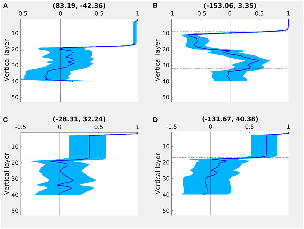
Figure 1. “True” correlation (Pearson correlation coefficient) profile (dark blue line) and 5th-to-95th percentile (light blue area) of 1,000 correlation profiles at (A) (83.19°E, –42.36°N), (B) (–153.06°E, 3.35°N), (C) (–28.31°E, 32.24°N), and (D) (–131.67°E, 40.38°N). The correlations are computed between SST and ocean temperature in the isopycnal coordinate from the same water column in January. The top (bottom) horizontal dashed line determines the threshold layer L in Equation (7) for step function with minimal (maximal) support.

We use the first isopycnal layer L (e.g., L = 19 in Figure 1A and L = 9 in Figure 1B, L = 17 in Figures 1C,D), below which (i.e., in layer L+1) correlations with SST are not significant, to define a step function:

$\begin{array}{ll}\rho (l)=\{\begin{array}{cc}1& \text{\hspace{1em}if }l\le L,\\ 0& \text{\hspace{1em}if }l>L,\end{array}& (7)\end{array}$

where l is the isopycnal layer index (starting from the surface). As such, the support of the step function (the domain where the function is not zero) is the interval [1, L] and the assimilation will not update the isopycnal temperature below the layer L.

Such an estimate is carried out for each water column (horizontal model grid) and for each calendar month. Figure 2 shows examples of the global maps of the threshold layer number L for different calendar months. As examples shown in Figure 1, L is located in the first few non-empty isopycnal layers below the mixed layer. As the ocean water density increases with latitudes and the constant potential densities are chosen for vertical discretization, there are more empty isopycnal layers below the mixed layer at higher latitudes (e.g., Figures 1A,C,D vs. 1B). It is the reason why L is higher in polar regions (e.g., Greenland, Barents, Labrador, Weddell and Ross Seas) and lower in the tropical regions (e.g., western tropical Pacific and Indian Oceans). The time-dependence of L is more obvious in the Arctic where sea ice influences ocean stratification, but less obvious at lower latitudes.

FIGURE 2

Figure 2. Global maps of the threshold layer number L (between 1 and 53) used to define step function with minimal support (Equation 7) for (A) March, (B) June, (C) September, and (D) December.

3.2. Step function with maximal support

At several locations (e.g., Figure 1B) we notice that correlation crosses zero at some intermediate layers but becomes rapidly significant again. In these cases, the step function with minimal support (Section 3.1) is not optimal as the deeper layer could potentially be updated by the assimilation thanks to their co-variability with the ocean surface. Such an oscillating structure is characteristic of a stratification change, typically with a higher (lower) SST linked to a shallower stratified (deeper) mixed layer and less heat exchange with the layer underneath causing a cold anomaly. Several other mechanisms can also cause a reemergence of correlation at depth, e.g., SST being a tracer of a front or deep water convection (e.g., Counillon et al., 2016).

In this scheme, we allow update until the last isopycnal layer for which the correlation is significant (i.e., L = 32 for Equation (7) in Figure 1B). Such a step function maximizes the impact of SST observations, and still removes insignificant correlations in deeper layers. Figure 3 presents the spatial distribution of the threshold layer L estimated with this approach. In most regions, the threshold layer is similar to the former step function (Figure 2). This corresponds to regions with relatively stable ocean stratification (e.g., Figures 1A,C,D). Nevertheless, the threshold layer L is much larger in the eastern tropical Pacific, North Atlantic SPG region and the Southern Ocean.

FIGURE 3

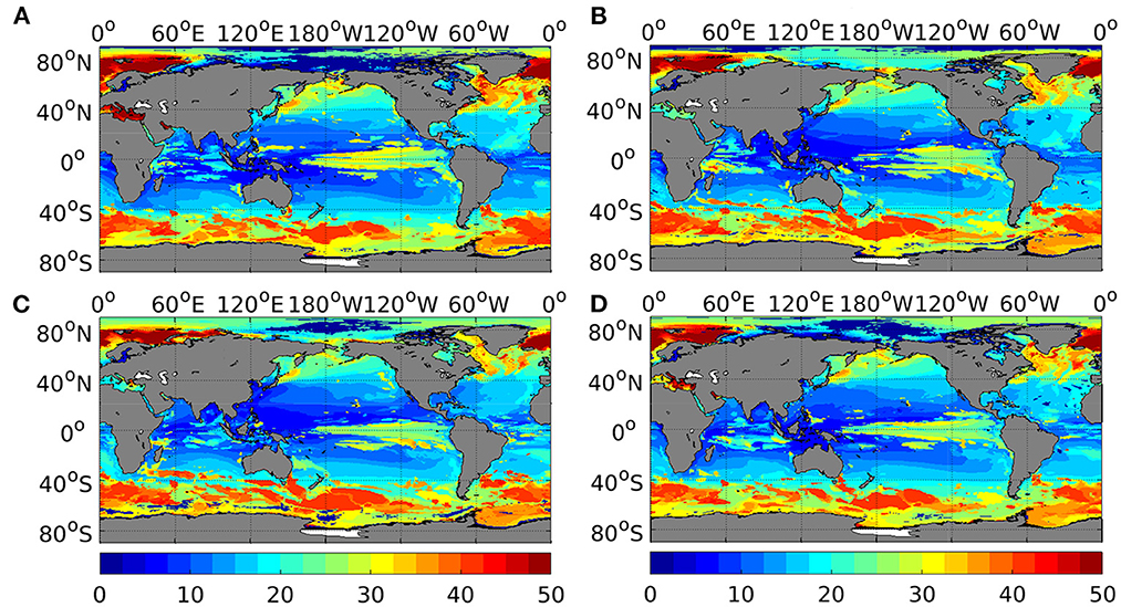
Figure 3. As in Figure 2, but for step function with maximal support (Section 3.2).

3.3. Smooth function

When applying localization in geoscience, typical covariances decay as a function of the distance and it is quite common to make use of a smooth tapering function (e.g., Gaspari and Cohn, 1999; Ménétrier et al., 2015a) to avoid discontinuity near the edge of the local domain (e.g., Sakov and Bertino, 2010; Wang et al., 2017). At the same time, the Gaussian-like tapering is distorting the covariance (Miyoshi et al., 2014). In this section, we make use of the covariance filtering theory developed by Ménétrier et al. (2015a) to define a smooth flattop tapering function. The flattop function gives more weights than the Gaussian-like function and leads to better use of surrounding observations in the analysis (e.g., Ménétrier et al., 2015a). This formulation is derived from the centered moment estimation theory and the optimal Schur filtering theory. It removes most of the sampling noise while keeping the signal of interest in the linear filtering of sample covariances. Please refer to Ménétrier et al. (2015a) for more details.

Assuming that the ensemble forecast error covariance is Gaussian, we employ Equation (64) of Ménétrier et al. (2015a) and simplify notations as follows:

$\begin{array}{ll}f(l)=\frac{m-1}{(m+1)(m-2)}\left[(m-1)-\frac{\text{𝔼}\left[{\text{P}}_{11}{\text{P}}_{ll}\right]}{\text{𝔼}\left[{\text{P}}_{1l}^2\right]}\right],& (8)\end{array}$

where l is the isopycnal layer number from the surface to the bottom, and m is the dynamic ensemble size (e.g., m = 30 in our case). The covariance matrix P is estimated from an ensemble of size m = 30. P₁₁ is the variance of SST, P_ll is the variance of temperature in the l-th layer and P_1l is the covariance between SST and temperature in l-th layer. 𝔼 is the expectation over 1,000 ensembles sampled from the large static ensemble (please refer to the beginning of Section 3.1). Note that when l = 1, f(l) is equal to $\frac{m-1}{m+1}$ that is less than 1. It is due to the fact that the sampling noise in variance is considered (Ménétrier et al., 2015a). As an example, blue circles in Figure 4 present the estimation from Equation (8). These estimates are noisy due to the fact that the number of ensemble-based estimates of the covariances, 315, is still relatively small (Miyoshi et al., 2014). The optimal localization function should have a flatter top than the Gaussian function (e.g., Ménétrier et al., 2015a), which leads to better use of surrounding observations in the analysis. We use a smooth flattop function to fit (Equation 8) as follows:

$\begin{array}{ll}\rho (l,L_1,L_2)=\{\begin{array}{ll}1\hfill & \text{\hspace{1em}if }l\le L_1,\hfill \\ \left[1+\text{cos}(\frac{l-L_1}{L_2-L_1}\pi )\right]/2\hfill & \text{\hspace{1em}if }{L}_1\le l\le L_2,\hfill \\ 0\hfill & \text{\hspace{1em}if }{L}_2\le l.\hfill \end{array}& (9)\end{array}$

FIGURE 4

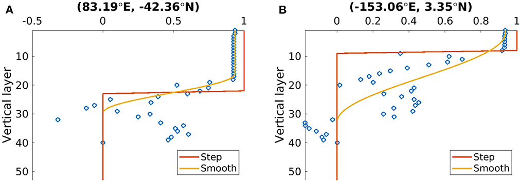
Figure 4. Tapering functions at (A) (83.19°E, –42.36°N) and (B) (–153.06°E, 3.35°N) in July. Blue circles are estimated from Equation (8). Yellow lines fit the blue circles with Equation (9). Red lines are step function with minimal support (Section 3.1).

Yellow lines of Figure 4 present the estimated smooth tapering functions. Compared to the step function with minimal support (red lines in Figure 4), the smooth function starts from $\frac{m-1}{m+1}$ rather than 1 to damp noise in variance. It smoothly decreases to zeros to damp noise in covariance at long distances. The two hyper-parameters of Equation (9): L₁ and L2 are tightly linked to the threshold layer numbers L in Sections 3.1, 3.2, respectively. As it is nicely exemplified in Figure 4, L₁ is typically smaller than L in the step function with minimal support and L₂ is larger than L in the step function with maximal support.

3.4. Multivariate consideration of tapering

We have above introduced the vertical localization functions for isopycnal temperature. We investigated also the vertical localization for salinity, velocity and layer thickness. For salinity, the tapering function is almost identical to that for temperature (not shown) because temperature and salinity are tightly linked by the target density of the isopycnal layer to which they belong.

The BLOM ocean model uses a barotropic/baroclinic mode splitting (Bentsen et al., 2013). As such the layer thickness and velocities combine both a signal that is correlated over the whole water column (barotropic) and another signal that is vertically local (baroclinic). Empirical correlation in layer thickness and velocities shows quite often a significant reemergence near the bottom layer (not shown in the paper). Furthermore, vertical localization leads to different linear weights for the different layers, implying that the linear properties are no longer preserved by the assimilation, e.g., geostrophy. For instance, this will make the sum of all layer thicknesses not consistent with the bottom pressure. The latter is challenging because its post-processing introduces a slow drift of global mass, heat and salt content (Mignac et al., 2015; Wang et al., 2016). We thus decided to employ vertical localization only for isopycnal temperature and salinity, but not for velocity and layer thickness.

4. Experimental design and metrics

We perform perfect twin experiments with NorCPM (Section 2) to demonstrate the benefit of vertical localization for the isopycnal coordinate model and to assess the different tapering functions (Section 3). In our idealized framework, the “truth” is known and produced from the same model but started from different initial conditions than used in the assimilation experiment. We assimilate synthetic SST observations generated from the “truth” and produce several reanalyzes over the period 1980–2010. The reanalysis performance is validated against the “truth”.

4.1. Twin experiment design

All experiments are forced by CMIP5 historical forcings (Taylor et al., 2012) before 2005 and the representative Concentration Pathway 8.5 (RCP8.5, van Vuuren et al., 2011) forcings after 2005. The CMIP5 historical forcings for 1850–2005 are based on observational variations in solar radiation (Lean et al., 2005; Wang et al., 2005), volcanic sulfate aerosol concentration (Ammann et al., 2003), GHG concentration (Lamarque et al., 2010), aerosol emission (Lamarque et al., 2010), and land-use (Hurtt et al., 2011).

The 30-member NorESM historical simulation without DA is referred to as FREE. Each member is started from a randomly selected initial condition from a stable pre-industrial simulation and integrates the ensemble from 1850 to 2014. The “truth” is spawned from member 1 of FREE by perturbing the SST of the initial conditions in January 1960 with spatially uncorrelated white noise with a standard deviation of 10⁻⁶ °C and then integrating it up to 2010 (henceforth referred to as TRUTH). We have verified that TRUTH and FREE's member 1 have fully diverged from each other before the start of the assimilation experiment in January 1980 (not shown in the paper). The global RMSE of FREE in reference to TRUTH is comparable to the model error in the real framework (Counillon et al., 2016, their Figure 1).

Synthetic SST observations are generated from monthly outputs of TRUTH by adding white noises. The amplitude of the noise is constructed to mimic that of realistic observations and set equal to the time-varying estimate of HadISST2 (i.e., the standard deviation of its 10 realizations). We also discard SST observations in sea ice cover regions, as in the real framework (Counillon et al., 2016).

We perform four NorCPM simulations with assimilation of synthetic monthly SST observations (i.e., reanalyzes) over 1980–2010 as follows:

• NOVL: Reanalysis without vertical localization,

• STEPmin: Reanalysis with the step function with minimal support (Section 3.1),

• STEPmax: Reanalysis with the step function with maximal support (Section 3.2),

• SMOOTH: Reanalysis with the smooth tapering function (Section 3.3).

All four reanalyzes start from January 1980 with the same initial conditions as FREE and have 30 ensemble members. The only difference in the configuration of these reanalyzes is the vertical localization setting.

4.2. Evaluation metrics

We measure simulation accuracy with the Mean Squared Skill Score (MSSS) and/or Root Mean Square Error (RMSE) difference (ΔRMSE). The MSSS is estimated from Mean Squared Error (MSE) against TRUTH. Following the formulations of Murphy (1988) and Goddard et al. (2013), the MSE is given as follows

$\begin{array}{ll}\text{MSE}={\displaystyle \sum _{j=1}^N}{w}_j{(x_j-x_j^{\text{t}})}^2,& (10)\end{array}$

where x_j is the state of the reanalysis (or FREE), $x_j^{\text{t}}$ is that of the TRUTH, and N is the number of states or observations. w_j is a weight for the index j and is set to $\frac{1}{N}$, but when computing the global MSE (e.g., Figure 5), w_j is a normalization term that considers the grid cell area. We take the FREE MSE as a reference to define the MSSS as follows:

$\begin{array}{ll}\text{MSSS}=1-\frac{{\text{MSE}}_{\text{r}}}{{\text{MSE}}_{\text{F}}},& (11)\end{array}$

where MSE_F is FREE's MSE and MSE_r is the MSE of reanalysis. In the case where MSE_r is equal to zero, the MSSS becomes one. The RMSE is the square root of the MSE. We take FREE as the reference and define ΔRMSE as the FREE RMSE minus the reanalysis RMSE. A positive MSSS (ΔRMSE) indicates that the reanalysis is more accurate than FREE and a negative MSSS (ΔRMSE) indicates that the reanalysis is less accurate than FREE. While ΔRMSE indicates error difference, the MSSS shows the proportion of error difference and FREE's error. Significant MSSS does not mean large ΔRMSE and vice versa. One advantage of the MSSS is that it is unitless. Thus, the MSSS is suitable for validation in depth (e.g., Figure 5), since the magnitude of error in the upper ocean is larger than that in the deeper ocean.

FIGURE 5

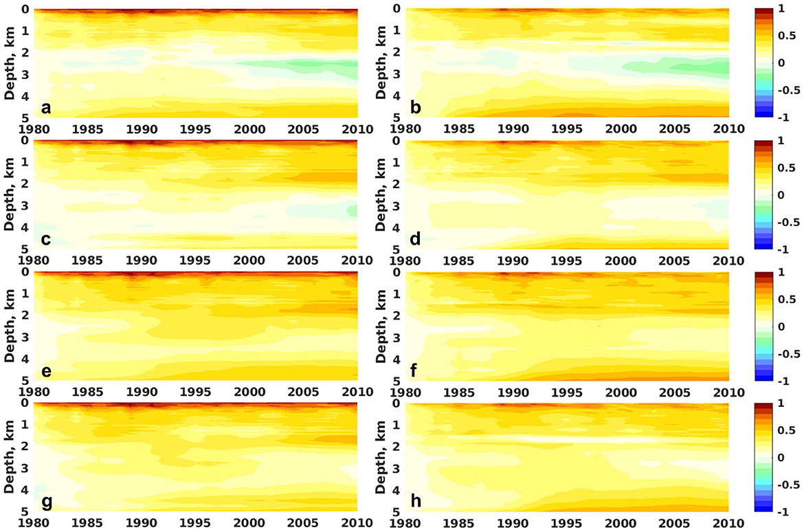
Figure 5. Hovmöller plots of MSSS of NOVL (row 1), STEPmin (row 2), STEPmax (row 3) and SMOOTH (row 4) in temperature (left column) and salinity (right column). Warm colors (positive MSSSs) indicate that the reanalysis overperforms FREE; cold colors (negative MSSSs) indicate that FREE overperforms the reanalysis.

5. Results and discussions

Figure 5 shows Hovmöller plots of MSSS of the reanalyzes in temperature and salinity. The reanalysis NOVL is more accurate than FREE in the top 2,000 m and below 4,000 m for both temperature and salinity, in particular temperature in the top 300 m. It is less accurate than FREE between 2,000 and 4,000 m in particular from 1995 onward (Figures 5a,b). The reanalysis STEPmin has similar MSSSs to NOVL in the top 1,000 m, higher MSSSs from 1,000 to 4,000 m in depth and lower MSSSs below 4,000 m in depth (Figures 5c,d). The reanalysis STEPmax notably alleviates the degradation between 2,000 and 4,000 m shown in NOVL (Figures 5a,b,e,f). The reanalysis STEPmax has higher MSSSs than STEPmin in both temperature and salinity (Figures 5c–f), which indicates the benefit of maximizing observation influence and updating the deeper layers (Figures 1, 3). The reanalysis SMOOTH is nearly as good as STEPmax, but its MSSSs are slightly lower.

Figure 6 shows the global maps of ΔRMSE in temperature and salinity over 0–1,000 m below the surface. The assimilation without vertical localization overall improves the model performance (Counillon et al., 2014, 2016), but leads to slight degradations in some regions (blue areas in Figures 6A,B), e.g., the Southern Ocean and tropical North Atlantic. There is a larger improvement in temperature than in salinity, because we assimilate SST and the two quantities are not tightly linked by the reference densities in the mixed layer (Section 2.1). The step function with minimal support significantly alleviates the degradation in these regions for temperature, but is less efficient for salinity (Figures 6C,D). The step function with maximal support leads to further improvements for salinity, e.g., the Southern Ocean (Figure 6F). Overall, the smooth tapering function yields relatively similar results to the step function with maximal support, but with significantly poorer performance for salinity near the Ross Sea.

FIGURE 6

Figure 6. Global maps of ΔRMSE of NOVL (row 1), STEPmin (row 2), STEPmax (row 3) and SMOOTH (row 4) in temperature (left column) and salinity (right column) over 0–1,000 m in depth. Warm colors (positive ΔRMSEs) indicate that the reanalysis overperforms FREE; cold colors (negative ΔRMSEs) indicate that FREE overperforms the reanalysis.

Figure 7 shows the global maps of ΔRMSE in temperature and salinity over 1,000-2,000 m below the surface. The significant improvement and degradation of the assimilation are mostly found in the middle latitudes (Figures 7A,B), which is related to ocean stratification and/or reemergence of covariance (Figures 2, 3). Vertical localization overall improves the reanalysis performance (Figures 7C–H). In particular, it reduces or alleviates the degradation found in NOVL, e.g., North Atlantic, North Pacific and Southern Ocean. Among different tapering functions, the step function with maximal support leads to the highest scores and the most stable performance (positive and negative anomalies). Regionally, STEPmax has the highest scores in temperature in the central North Pacific and North Atlantic, and in salinity in the North Atlantic.

FIGURE 7

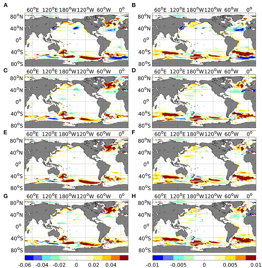
Figure 7. As in Figure 6, but for temperature (left column) and salinity (right column) over 1,000–2,000 m in depth.

The assimilation without vertical localization leads to a large degradation in temperature and salinity below 2,000 m (Figures 8A,B), e.g., in the North Pacific, North Atlantic and Southern Ocean. Note that the geographic patterns in temperature and salinity mostly coincide with each other due to the feature of density vertical coordinate. Vertical localization overall improves the reanalysis performance (Figures 8C–H). It notably removes degradation in temperature and salinity in the North Pacific and mitigates degradation in the North Atlantic. However, STEPmin has a degradation in the Southern Ocean. Since we discard sea ice-covered SST observations (Section 4.1), there is almost no DA update in the sea ice cover area (not shown in the paper). The changes are thus remote and mostly caused by the changes in the Circumpolar Deep Water (Carter et al., 2008), due to a significant relation between SST and the deep water masses. A piece of evidence is that the step functions with minimal and maximal support were substantially different (Figures 2, 3). The latter leads to better performance (STEPmax, Figures 8E,F) in the Southern Ocean. STEPmax has higher scores (Figures 8E,F) than STEPmin. It is worth noting that using a deeper threshold layer alleviates degradation in the eastern subtropical North Atlantic where STEPmin has degradation. It may be related to improved performance in the Mediterranean Sea. The relatively saline water flows out of the Mediterranean Sea through the Strait of Gibraltar (called the Mediterranean outflow, Price et al., 1993) and quickly sinks and spreads westward around a depth of 1,000 m. The Mediterranean Water can be detected several 1,000 km west of the Strait of Gibraltar. It may also be related to the circulation changes in the North Atlantic (Bozec et al., 2011), e.g., the SPG region (Figures 2, 3). There, SST can skillfully update deep water masses in SPG region (i.e., deep water convection, Counillon et al., 2016), which influences the subtropical North Atlantic (e.g., Koul et al., 2020). The reanalysis SMOOTH has similar geographic patterns to STEPmax (Figures 8E–H) but with slightly poorer performance for temperature near the Ross Sea.

FIGURE 8

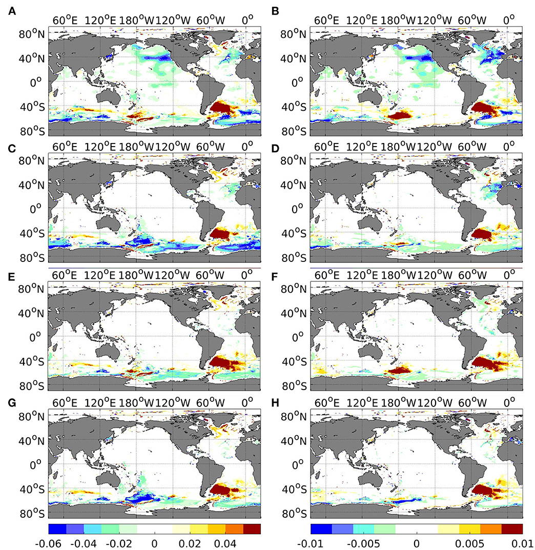
Figure 8. As in Figure 6, but for temperature (left column) and salinity (right column) below 2,000 m in depth.

As found in the paragraphs above, the step function with maximal support (i.e., a large localization radius) overall outperforms the smooth tapering function for both temperature and salinity. That is because of the key feature of isopycnal coordinate ocean models. There is microscopic exchange across isopycnal coordinates. The covariance formulated in isopycnal coordinates has a significant discontinuity in the vertical layers (e.g., near the bottom of the mixed layer Counillon et al., 2016, the left panels of their Figure 9). We foresee that a smooth tapering function would be most suitable for the models in geopotential coordinates. Furthermore, since our findings are based on an isopycnal coordinate model (i.e., NorCPM), we expect that our findings can be applied to other isopycnal or hybrid ocean models, e.g., HYCOM (Bleck, 2002) and MOM6 (Adcroft et al., 2019). We use the EnKF in this study, but the proposed approach can be applied to the ensemble Optimal Interpolation (Evensen, 2003).

6. Conclusions and perspectives

We introduced vertical localization in the isopycnal coordinate to limit the degradation in the interior ocean that emerges when assimilating SST with an ensemble-based DA method and a finite ensemble size. We proposed three schemes which vary spatially and for each calendar month: a step function with a small localization radius, a step function with a large localization radius and a smooth flattop tapering function. The three schemes rely on a very long pre-industrial simulation to perform statistical significance tests. They were tested in identical twin experiments with NorCPM and applied for both isopycnal temperature and salinity. It is found that vertical localization greatly reduces the degradation and improves the overall accuracy of the climate reanalysis, in particular between 2,000 and 4,000 m and in the North Pacific and the North Atlantic. Among the three schemes, the step function with large localization radius (i.e., that maximizes the impact of observations) outperforms the other schemes for both temperature and salinity. These results also confirm that a vertically continuous analysis update is not a requirement for isopycnal coordinate models.

The evidence of the benefit of vertical localization has been demonstrated in idealized twin experiments. There is a need to further verify these findings in the real framework (i.e., assimilation of real SST observations). One big challenge in the real framework is the model bias, in particular for fully-coupled Earth system model (Richter, 2015). Models are attracted to their biased climatological states after assimilation (i.e., model drift). Furthermore, the model drift in the observed variables is propagated to the non-observed variables, which leads to slow degradation of the system through the consecutive assimilation cycle. Due to that, NorCPM (like many other Earth system models) performs anomaly assimilation (Weber et al., 2015) where the observed anomaly (calculated relative to a reference climatology of observation) is assimilated (Counillon et al., 2016; Wang et al., 2017; Bethke et al., 2021). The anomaly assimilation does not show any detrimental effects on model climatology (Bethke et al., 2021). Therefore, we foresee that the findings of this study will be very beneficial for NorCPM to reconstruct the climate, e.g., over the period of 1850-present when SST observations are a critical data set. Our findings can also be applied to other isopycnal or hybrid ocean models (e.g., HYCOM Bleck, 2002 and MOM6 Adcroft et al., 2019) to improve their reanalysis products (e.g., Sakov et al., 2012). In Bethke et al. (2018), the degradation in the tropical North Atlantic was found to lead to drift in the decadal prediction in the North Atlantic SPG region. It would be interesting to assess the impact of vertical localization on decadal prediction skill.

The formulations of vertical localization proposed were relatively simple and could be refined. We have seen that continuity of the analysis update in the vertical was not a requirement as isopycnal temperature and salinity are updated along the density line, which ensures dynamical stability. One could test a version of the tapering function that only updates layers where correlations are statically significant (e.g., multi-step function). Also, the current formulation has been specifically tailored for SST assimilation but also needs to be adapted for hydrographic profile assimilation. We foresee that a similar methodology could be applied but in both directions (upward and downward).

The current vertical localization is applied to isopycnal temperature and salinity. Applying vertical localization to layer thickness and velocity is more challenging (Section 3.4). The mode of variability (barotropic and baroclinic) in the water column could be decomposed as in the model code (mode splitting), and could apply vertical localization only on the baroclinic part of the velocity and layer thickness. However, we foresee that sampling errors may interfere with the mode decomposition and cause large instabilities.

Finally, there are different manners to address sampling errors. The use of hybrid covariance (Hamill and Snyder, 2000) is another technique and it is currently being tested in NorCPM. It is expected that when using hybrid covariance, sampling errors will be reduced and the vertical localization scheme needs to be adapted (Ménétrier and Auligné, 2015; Carrió et al., 2021).

Data availability statement

The raw data supporting the conclusions of this article will be shared by the authors via personal communications.

Author contributions

YW coordinated the study and the writing of this article. YW and FC estimated the localization functions and performed the simulation experiments. All co-authors contributed to the analysis of the simulation experiments and the writing of this article.

Funding

This study was supported by the Research Council of Norway (Grant Nos. 301396 and 270061) and the Trond Mohn Foundation under project number BFS2018TMT01.

Acknowledgments

We thank UNINETT Sigma2 for computing and storage resources (nn9039k and ns9039k).

Conflict of interest

The authors declare that the research was conducted in the absence of any commercial or financial relationships that could be construed as a potential conflict of interest.

Publisher's note

All claims expressed in this article are solely those of the authors and do not necessarily represent those of their affiliated organizations, or those of the publisher, the editors and the reviewers. Any product that may be evaluated in this article, or claim that may be made by its manufacturer, is not guaranteed or endorsed by the publisher.

References

Adcroft, A., Anderson, W., Balaji, V., Blanton, C., Bushuk, M., Dufour, C. O., et al. (2019). The gfdl global ocean and sea ice model om4.0: model description and simulation features. J. Adv. Model. Earth Syst. 11, 3167–3211. doi: 10.1029/2019MS001726

CrossRef Full Text | Google Scholar

Ammann, C. M., Meehl, G. A., Washington, W. M., and Zender, C. S. (2003). A monthly and latitudinally varying volcanic forcing dataset in simulations of 20th century climate. Geophys. Res. Lett. 30, 16875. doi: 10.1029/2003GL016875

CrossRef Full Text | Google Scholar

Balmaseda, M., and Anderson, D. (2009). Impact of initialization strategies and observations on seasonal forecast skill. Geophys. Res. Lett. 36, 35561. doi: 10.1029/2008GL035561

CrossRef Full Text | Google Scholar

Bentsen, M., Bethke, I., Debernard, J. B., Iversen, T., Kirkevåg, A., Seland, O., et al. (2013). The norwegian earth system model, NorESM1-Part 1: description and basic evaluation of the physical climate. Geosci. Model Dev. 6, 687–720. doi: 10.5194/gmd-6-687-2013

CrossRef Full Text | Google Scholar

Bethke, I., Wang, Y., Counillon, F., Keenlyside, N., Kimmritz, M., Fransner, F., et al. (2021). Norcpm1 and its contribution to cmip6 dcpp. Geosci. Model Dev. 14, 7073–7116. doi: 10.5194/gmd-14-7073-2021

CrossRef Full Text | Google Scholar

Bethke, I., Wang, Y., Counillon, F., Kimmritz, M., Langehaug, H., Bentsen, M., et al. (2018). “Subtropical north atlantic preconditioning key to skillful subpolar gyre prediction,” in Second International Conference on Seasonal to Decadal Prediction, Boulder.

Google Scholar

Billeau, S., Counillon, F., Keenlyside, N., and Bertino, L. (2016). Impact of changing the assimilation cycle: centered vs. staggered, snapshot vs monthly averaged. NERSC Technical Report 400, Nansen Environmental and Remote Sensing Center.

Google Scholar

Bleck, R. (2002). An oceanic general circulation model framed in hybrid isopycnic-Cartesian coordinates. Ocean Model. 4, 55–88. doi: 10.1016/S1463-5003(01)00012-9

CrossRef Full Text | Google Scholar

Bleck, R., Rooth, C., Hu, D., and Smith, L. T. (1992). Salinity-driven thermocline transients in a wind- and thermohaline-forced isopycnic coordinate model of the North Atlantic. J. Phys. Oceanogr. 22, 1486–1505. doi: 10.1175/1520-0485(1992)022<1486:SDTTIA>2.0.CO;2

CrossRef Full Text | Google Scholar

Bozec, A., Lozier, M. S., Chassignet, E. P., and Halliwell, G. R. (2011). On the variability of the mediterranean outflow water in the north atlantic from 1948 to 2006. J. Geophys. Res. Oceans 116, 7191. doi: 10.1029/2011JC007191

CrossRef Full Text | Google Scholar

Brune, S., Nerger, L., and Baehr, J. (2015). Assimilation of oceanic observations in a global coupled Earth system model with the SEIK filter. Ocean Model. 96, 254–264. doi: 10.1016/j.ocemod.2015.09.011

CrossRef Full Text | Google Scholar

Carrassi, A., Bocquet, M., Bertino, L., and Evensen, G. (2018). Data assimilation in the geosciences: an overview of methods, issues, and perspectives. Wiley Interdisc. Rev. Clim. Change 9, e535. doi: 10.1002/wcc.535

CrossRef Full Text | Google Scholar

Carri,ó, D. S., Bishop, C. H., and Kotsuki, S. (2021). Empirical determination of the covariance of forecast errors: an empirical justification and reformulation of hybrid covariance models. Q. J. R. Meteorol. Soc. 147, 2033–2052. doi: 10.1002/qj.4008

CrossRef Full Text | Google Scholar

Carter, L., McCave, I. N., and Wiliams, M. J. M. (2008). “Circulation and water masses of the southern ocean: A review,” in Developments in Earth and Environmental Sciences, Vol. 8, eds F. Florindo and M. Siegert (Elsevier), 85–114. doi: 10.1016/S1571-9197(08)00004-9

CrossRef Full Text | Google Scholar

Counillon, F., and Bertino, L. (2009). Ensemble optimal interpolation: multivariate properties in the gulf of mexico. Tellus A 61, 296–308. doi: 10.1111/j.1600-0870.2008.00383.x

CrossRef Full Text | Google Scholar

Counillon, F., Bethke, I., Keenlyside, N., Bentsen, M., Bertino, L., and Zheng, F. (2014). Seasonal-to-decadal predictions with the ensemble Kalman filter and the Norwegian Earth System Model: a twin experiment. Tellus A 66, 1–21. doi: 10.3402/tellusa.v66.21074

CrossRef Full Text | Google Scholar

Counillon, F., Keenlyside, N., Bethke, I., Wang, Y., Billeau, S., Shen, M. L., et al. (2016). Flow-dependent assimilation of sea surface temperature in isopycnal coordinates with the Norwegian Climate Prediction Model. Tellus A 68, 1–17. doi: 10.3402/tellusa.v68.32437

CrossRef Full Text | Google Scholar

Craig, A. P., Vertenstein, M., and Jacob, R. (2012). A new flexible coupler for earth system modeling developed for CCSM4 and CESM1. Int. J. High Perform. Comput. Appl. 26, 31–42. doi: 10.1177/1094342011428141

CrossRef Full Text | Google Scholar

Dee, D. P., Uppala, S. M., Simmons, A. J., Berrisford, P., Poli, P., Kobayashi, S., et al. (2011). The ERA-Interim reanalysis: configuration and performance of the data assimilation system. Q. J. R. Meteorol. Soc. 137, 553–597. doi: 10.1002/qj.828

CrossRef Full Text | Google Scholar

Evensen, G. (2003). The Ensemble Kalman Filter: theoretical formulation and practical implementation. Ocean Dyn. 53, 343–367. doi: 10.1007/s10236-003-0036-9

CrossRef Full Text | Google Scholar

Eyring, V., Bony, S., Meehl, G. A., Senior, C. A., Stevens, B., Stouffer, R. J., et al. (2016). Overview of the Coupled Model Intercomparison Project Phase 6 (CMIP6) experimental design and organization. Geosci. Model Dev. 9, 1937–1958. doi: 10.5194/gmd-9-1937-2016

CrossRef Full Text | Google Scholar

Gaspari, G., and Cohn, S. E. (1999). Construction of correlatin functions in two and three dimensions. Q. J. R. Meteorol. Soc., 125, 723–757. doi: 10.1002/qj.49712555417

CrossRef Full Text | Google Scholar

Gavart, M., and Mey, P. D. (1997). Isopycnal eofs in the azores current region: a statistical tool fordynamical analysis and data assimilation. J. Phys. Oceanogr. 27, 2146–2157. doi: 10.1175/1520-0485(0)027<2146:IEITAC>2.0.CO;2

CrossRef Full Text | Google Scholar

Gent, P. R., Danabasoglu, G., Donner, L. J., Holland, M. M., Hunke, E. C., Jayne, S. R., et al. (2011). The community climate system model version 4. J. Clim. 24, 4973–4991. doi: 10.1175/2011JCLI4083.1

CrossRef Full Text | Google Scholar

Goddard, L., Kumar, A., Solomon, A., Smith, D., Boer, G., Gonzalez, P., et al. (2013). A verification framework for interannual-to-decadal predictions experiments. Clim. Dyn. 40, 245–272. doi: 10.1007/s00382-012-1481-2

CrossRef Full Text | Google Scholar

Halem, M., and Dlouhy, R. (1984). Observing system simulation experiments related to space-borne lidar wind profiling. part 1: Forecast impacts of highly idealized observing systems. Res. Rev. 1983, 19840013984.

Google Scholar

Hamill, T. M., and Snyder, C. (2000). A hybrid ensemble kalman filter-3d variational analysis scheme. Mon. Weather Rev. 128, 2905–2919. doi: 10.1175/1520-0493(2000)128<2905:AHEKFV>2.0.CO;2

CrossRef Full Text | Google Scholar

Hamill, T. M., Whitaker, J. S., and Snyder, C. (2001). Distance-dependent filtering of background error covariance estimates in an ensemble kalman filter. Mon. Weather Rev. 129, 2776–2790. doi: 10.1175/1520-0493(2001)129<2776:DDFOBE>2.0.CO;2

CrossRef Full Text | Google Scholar

Holland, M. M., Bailey, D. A., Briegleb, B. P., Light, B., and Hunke, E. (2012). Improved sea ice shortwave radiation physics in CCSM4: the impact of melt ponds and aerosols on arctic sea ice. J. Clim. 25, 1413–1430. doi: 10.1175/JCLI-D-11-00078.1

CrossRef Full Text | Google Scholar

Houtekamer, P. L., and Mitchell, H. L. (2001). A sequential ensemble kalman filter for atmospheric data assimilation. Mon. Weather Rev. 129, 123–137. doi: 10.1175/1520-0493(2001)129<0123:ASEKFF>2.0.CO;2

CrossRef Full Text | Google Scholar

Hurtt, G. C., Chini, L. P., Frolking, S., Betts, R. A., Feddema, J., Fischer, G., et al. (2011). Harmonization of land-use scenarios for the period 1500-2100: 600 years of global gridded annual land-use transitions, wood harvest, and resulting secondary lands. Clim. Chang. 109, 117. doi: 10.1007/s10584-011-0153-2

CrossRef Full Text | Google Scholar

Kalnay, E., Kanamitsu, M., Kistler, R., Collins, W., Deaven, D., Gandin, L., et al. (1996). The ncep/ncar 40-year reanalysis project. Bull. Am. Meteorol. Soc. 77, 437–471. doi: 10.1175/1520-0477(1996)077<0437:TNYRP>2.0.CO;2

CrossRef Full Text | Google Scholar

Karspeck, A. R., Yeager, S., Danabasoglu, G., Hoar, T., Collins, N., Raeder, K., et al. (2013). An ensemble adjustment kalman filter for the CCSM4 ocean component. J. Clim. 26, 7392–7413. doi: 10.1175/JCLI-D-12-00402.1

CrossRef Full Text | Google Scholar

Kimmritz, M., Counillon, F., Smedsrud, L. H., Bethke, I., Keenlyside, N., Ogawa, F., et al. (2019). Impact of ocean and sea ice initialisation on seasonal prediction skill in the arctic. J. Adv. Model. Earth Syst. 11, 4147–4166. doi: 10.1029/2019MS001825

CrossRef Full Text | Google Scholar

Kirkevåg, A., Iversen, T., Seland, Ø., Hoose, C., Kristjánsson, J. E., Struthers, H., et al. (2013). Aerosol-climate interactions in the norwegian earth system-noresm1-m. Geosci. Model Dev. 6, 207–244. doi: 10.5194/gmd-6-207-2013

PubMed Abstract | CrossRef Full Text | Google Scholar

Koul, V., Tesdal, J., Bersch, M., Hatun, H., Brune, S., Borchert, L., et al. (2020). Unraveling the choice of the north atlantic subpolar gyre index. Sci Rep 10, 1005. doi: 10.1038/s41598-020-57790-5

PubMed Abstract | CrossRef Full Text | Google Scholar

Laloyaux, P., de Boisseson, E., Balmaseda, M., Bidlot, J.-R., Broennimann, S., Buizza, R., et al. (2018a). Cera-20c: a coupled reanalysis of the twentieth century. J. Adv. Model. Earth Syst. 10, 1172–1195. doi: 10.1029/2018MS001273

CrossRef Full Text | Google Scholar

Laloyaux, P., Frolov, S., Ménétrier, B., and Bonavita, M. (2018b). Implicit and explicit cross-correlations in coupled data assimilation. Q. J. R. Meteorol. Soc. 144, 1851–1863. doi: 10.1002/qj.3373

CrossRef Full Text | Google Scholar

Lamarque, J.-F., Bond, T. C., Eyring, V., Granier, C., Heil, A., Klimont, Z., et al. (2010). Historical (1850-2000) gridded anthropogenic and biomass burning emissions of reactive gases and aerosols: methodology and application. Atmospheric Chem. Phys. 10, 7017–7039. doi: 10.5194/acp-10-7017-2010

CrossRef Full Text | Google Scholar

Lawrence, D. M., Oleson, K. W., Flanner, M. G., Thornton, P. E., Swenson, S. C., Lawrence, P. J., et al. (2011). Parameterization improvements and functional and structural advances in version 4 of the community land model. J. Adv. Model. Earth Syst. 3, M03001. doi: 10.1029/2011MS000045

CrossRef Full Text | Google Scholar

Lean, J., Rottman, G., Harder, J., and Kopp, G. (2005). Sorce contributions to new understanding of global change and solar variability. Solar Phys. 230, 27–53. doi: 10.1007/s11207-005-1527-2

CrossRef Full Text | Google Scholar

Ménétrier, B., and Auligné, T. (2015). Optimized localization and hybridization to filter ensemble-based covariances. Mon. Weather Rev. 143, 3931–3947. doi: 10.1175/MWR-D-15-0057.1

CrossRef Full Text | Google Scholar

Ménétrier, B., Montmerle, T., Michel, Y., and Berre, L. (2015a). Linear filtering of sample covariances for ensemble-based data assimilation. Part i: optimality criteria and application to variance filtering and covariance localization. Mon. Weather Rev. 143, 1622–1643. doi: 10.1175/MWR-D-14-00157.1

CrossRef Full Text | Google Scholar

Ménétrier, B., Montmerle, T., Michel, Y., and Berre, L. (2015b). Linear filtering of sample covariances for ensemble-based data assimilation. Part ii: application to a convective-scale nwp model. Mon. Weather Rev. 143, 1644–1664. doi: 10.1175/MWR-D-14-00156.1

CrossRef Full Text | Google Scholar

Mignac, D., Tanajura, C. a,. S, Santana, a,. N., Lima, L. N., and Xie, J. (2015). Argo data assimilation into HYCOM with an EnOI method in the Atlantic Ocean. Ocean Sci. 11, 195–213. doi: 10.5194/os-11-195-2015

CrossRef Full Text | Google Scholar

Miyoshi, T., Kondo, K., and Imamura, T. (2014). The 10,240-member ensemble kalman filtering with an intermediate agcm. Geophys. Res. Lett. 41, 5264–5271. doi: 10.1002/2014GL060863

CrossRef Full Text | Google Scholar

Mulholland, D. P., Laloyaux, P., Haines, K., and Balmaseda, M. A. (2015). Origin and impact of initialization shocks in coupled atmosphere-ocean forecasts. Mon. Weather Rev. 143, 4631–4644. doi: 10.1175/MWR-D-15-0076.1

CrossRef Full Text | Google Scholar

Murphy, A. H. (1988). Skill scores based on the mean square error and their relationships to the correlation coefficient. Mon. Weather Rev. 116, 2417–2424. doi: 10.1175/1520-0493(1988)116<2417:SSBOTM>2.0.CO;2

CrossRef Full Text | Google Scholar

O'Kane, T. J., Sandery, P. A., Kitsios, V., Sakov, P., Chamberlain, M. A., Collier, M. A., et al. (2021). Cafe60v1: a 60-year large ensemble climate reanalysis. Part i: system design, model configuration, and data assimilation. J. Clim. 34, 5153–5169. doi: 10.1175/JCLI-D-20-0974.1

CrossRef Full Text | Google Scholar

Oleson, K. W., Lawrence, D. M., Bonan, G. B., Flanner, M. G., Kluzek, E., Lawrence, P. J., et al. (2010). Technical Description of version 4.0 of the Community Land Model (CLM). Technical Report. NCAR/TN-478+STR. National Center for Atmospheric Research, Boulder, Colorado, USA.

Google Scholar

Ott, E., Hunt, B. R., Szunyogh, I., Zimin, A. V., Kostelich, E. J., Corazza, M., et al. (2004). A local ensemble kalman filter for atmospheric data assimilation. Tellus A 56, 415–428. doi: 10.3402/tellusa.v56i5.14462

PubMed Abstract | CrossRef Full Text | Google Scholar

Price, J. F., Baringer, M. O., Lueck, R. G., Johnson, G. C., Ambar, I., Parrilla, G., et al. (1993). Mediterranean outflow mixing and dynamics. Science 259, 1277–1282. doi: 10.1126/science.259.5099.1277

PubMed Abstract | CrossRef Full Text | Google Scholar

Rayner, N. A., Parker, D. E., Horton, E. B., Folland, C. K., Alexander, L. V., Rowell, D. P., et al. (2003). Global analyses of sea surface temperature, sea ice, and night marine air temperature since the late nineteenth century. J. Geophys. Res. Atmosph. 108, 2670. doi: 10.1029/2002JD002670

CrossRef Full Text | Google Scholar

Richter, I. (2015). Climate model biases in the eastern tropical oceans: causes, impacts and ways forward. Wiley Interdisc. Rev. Clim. Change 6, 345–358. doi: 10.1002/wcc.338

CrossRef Full Text | Google Scholar

Sakov, P., and Bertino, L. (2010). Relation between two common localisation methods for the EnKF. Comput. Geosci. 15, 225–237. doi: 10.1007/s10596-010-9202-6

CrossRef Full Text | Google Scholar

Sakov, P., Counillon, F., Bertino, L., Lisæter, K. A., Oke, P. R., and Korablev, A. (2012). TOPAZ4: an ocean-sea ice data assimilation system for the North Atlantic and Arctic. Ocean Sci. 8, 633–656. doi: 10.5194/os-8-633-2012

CrossRef Full Text | Google Scholar

Sakov, P., and Oke, P. R. (2008). A deterministic formulation of the ensemble Kalman filter: an alternative to ensemble square root filters. Tellus A 60, 361–371. doi: 10.1111/j.1600-0870.2007.00299.x

CrossRef Full Text | Google Scholar

Srinivasan, A., Chassignet, E. P., Bertino, L., Brankart, J. M., Brasseur, P., Chin, T. M., et al. (2011). A comparison of sequential assimilation schemes for ocean prediction with the HYbrid Coordinate Ocean Model (HYCOM): twin experiments with stati c forecast error covariances. Ocean Model. 37, 85–111. doi: 10.1016/j.ocemod.2011.01.006

CrossRef Full Text | Google Scholar

Taylor, K. E., Stouffer, R. J., and Meehl, G. A. (2012). An overview of CMIP5 and the experiment design. Bull. Am. Meteorol. Soc. 93, 485–498. doi: 10.1175/BAMS-D-11-00094.1

PubMed Abstract | CrossRef Full Text | Google Scholar

van Vuuren, D. P., Edmonds, J., Kainuma, M., Riahi, K., Thomson, A., Hibbard, K., et al. (2011). The representative concentration pathways: an overview. Clim Change 109, 5. doi: 10.1007/s10584-011-0148-z

CrossRef Full Text | Google Scholar

Vertenstein, M., Craig, T., Middleton, A., Feddema, D., and Fischer, C. (2012). CESM1.0.3 User Guide. Available online at: http://www.cesm.ucar.edu/models/cesm1.0/cesm/cesm_doc_1_0_4/ug.pdf (accessed January 23, 2015).

Google Scholar

Wang, Y., Counillon, F., and Bertino, L. (2016). Alleviating the bias induced by the linear analysis update with an isopycnal ocean model. Q. J. R. Meteorol. Soc. 142, 1064–1074. doi: 10.1002/qj.2709

CrossRef Full Text | Google Scholar

Wang, Y., Counillon, F., Bethke, I., Keenlyside, N., Bocquet, M., and Shen, M.-L. (2017). Optimising assimilation of hydrographic profiles into isopycnal ocean models with ensemble data assimilation. Ocean Model. 114, 33–44. doi: 10.1016/j.ocemod.2017.04.007

CrossRef Full Text | Google Scholar

Wang, Y., Counillon, F., Keenlyside, N., Svendsen, L., Gleixner, S., Kimmritz, M., et al. (2019). Seasonal predictions initialised by assimilating sea surface temperature observations with the EnKF. Clim. Dyn. 53, 5777–5797. doi: 10.1007/s00382-019-04897-9

CrossRef Full Text | Google Scholar

Wang, Y.-M., Lean, J. L., and Sheeley Jr, N. R. (2005). Modeling the sun's magnetic field and irradiance since 1713. Astrophys. J. 625, 522–538. doi: 10.1086/429689

CrossRef Full Text | Google Scholar

Weber, R. J. T., Carrassi, A., and Doblas-Reyes, F. J. (2015). Linking the anomaly initialization approach to the mapping paradigm: a proof-of-concept study. Mon. Weather Rev. 143, 4695–4713. doi: 10.1175/MWR-D-14-00398.1

CrossRef Full Text | Google Scholar

Zhang, S., Harrison, M. J., Rosati, A., and Wittenberg, A. (2007). System design and evaluation of coupled ensemble data assimilation for global oceanic climate studies. Mon. Weather Rev. 135, 3541–3564. doi: 10.1175/MWR3466.1

CrossRef Full Text | Google Scholar

Zuo, H., Balmaseda, M. A., Tietsche, S., Mogensen, K., and Mayer, M. (2019). The ECMWF operational ensemble reanalysis-analysis system for ocean and sea ice: a description of the system and assessment. Ocean Sci. 15, 779–808. doi: 10.5194/os-15-779-2019

CrossRef Full Text | Google Scholar