Historical Observations for Improving Reanalyses

Historical reanalyses have become a widely used resource for analyzing weather and climate processes and their changes over time. In this article I explore how further historical observations could support reanalyses and lead to products that reach further back in time or have a better quality. Using an off-line Ensemble Kalman Filter I estimate improvements arising from assimilating additional observations into the ensemble of the “Twentieth Century Reanalysis” Version 3 (20CRv3). I demonstrate this for three case studies and evaluate them using independent data and a leave-one-out approach. For Europe in 1807, assimilating additional pressure data improves the skill for pressure but slightly decreases it for temperature, while assimilating temperature data, a variable that is not assimilated in 20CRv3, improves the skill for temperature but slightly decreases it for pressure. Assimilating both leads to substantially increased skill in a leave-one-out approach. For Sub-Saharan Africa in 1877/78, assimilating ship-based pressure observations as well as land station data, albeit extremely sparse, leads to a slight improvement over the entire domain. Finally, for Europe in 1926/27, assimilating upper air and total column ozone observations both lead to improvements in geopotential height and wind in the middle troposphere and in total column ozone, but with little or no effect in the lower troposphere. This is because 20CRv3 is already close to perfect over Europe in this period. The article shows how additional observations could improve historical reanalyses. A backward extension to the 1780s seems possible, but further data rescue efforts are necessary. For some applications, improved fields as generated by the offline assimilation presented in this study could be useful.

Introduction

In 2006, Compo et al. (2006) demonstrated the feasibility of a dynamical atmospheric reanalysis based only on surface information. This allowed reanalysis data sets to be extended backward in time by a century compared with conventional reanalysis. The “Twentieth Century Reanalysis,” which was subsequently produced (Compo et al., 2011), has become a widely used data set. Its latest version (Slivinski et al., 2019) reaches as far back as 1806. Further surface-based reanalyses have been produced by the European Center for Medium Range Weather Forecasts (ECMWF), namely ERA-20C (Poli et al., 2018) and CERA20C (Laloyaux et al., 2018).

Although all products are successfully and widely used, they are not without problems. The quality deteriorates particularly when going far back in time (Slivinski et al., 2020). Some regions are very poorly constrained, and the question how far upper-level fields in this reanalysis can be trusted is not well-studied. In this article, I address the potential of additional observations for improving next generation long reanalyses.

Tremendous efforts have been undertaken in the past years to increase global coverage of historical weather data, coordinated in the Atmospheric Circulation Reconstructions over the Earth initiative (ACRE, Allan et al., 2011). These efforts now provide a steady stream of new data, supported through Copernicus Climate Change Service (C3S) Data Rescue Service (Brönnimann et al., 2018a). A workflow through the C3S database (Thorne et al., 2017; Noone et al., 2021) is established, that will facilitate future reanalyses. But what data brings the most benefit? How should data rescue efforts be prioritized?

In this article I address this question by performing experiments using the existing 20CRv3 reanalysis, into which I assimilate additional observations in an off-line approach. This does not quantify the full potential of the additional data, as their effect on the next forecast step is not included. However, it provides first answers as to where and when observations are particularly valuable.

This framework is used for several examples. The first, concerning the year 1807 over Europe, addresses the value of additional pressure observations—but also temperature observations, which are not assimilated in 20CRv3—from land stations in a period with very sparse data. The summer of that year was extremely warm over Europe (Casty et al., 2005) and at the same time this year is at the very beginning of 20CRv3 and therefore is perhaps suitable for showing the potential. In the second example, the value of additional marine data is studied for the case of the climate anomalies over Africa during the El Niño year of 1877/1878. This was one of the most momentous climate events in history (Singh et al., 2018). Using a period in the 1920s, I then address the value of assimilating upper air data and even total column ozone data (the period was chosen based on ozone data availability). Before going into these examples, however, I address the question how far back a global dynamical reanalysis could possibly be extended, considering the data that are known to have been measured (though not necessarily imaged or digitized).

The article is structured as follows. First the common data sets (20CRv3) and the common methodology, the offline Ensemble Kalman Filter, are introduced. Then the results for the four cases are presented. In the discussion I briefly also address the role of other observations such as oceanic data, data from the land surface, or forcing data. The article ends with brief conclusions.

Data and Methods

The Twentieth Century Reanalysis

The Twentieth Century Reanalysis (20CRv3, Slivinski et al., 2019) is a global dynamical reanalysis reaching back to 1806. It has 80 members with a spatial resolution of 1° × 1°. For this article I use fields at 12 UTC for all cases and I use all 80 members.

Note that the state vector for the assimilation problem in this article does not cover the full model state, which is not necessary as the analysis is not cycled to the model. The state vector only needs the information required to model the observations, plus any desired output field that is of interest for the analysis. Therefore, the variables used in this study encompass 2 m temperature, mean sea-level pressure, u and v wind at 850 and 500 hPa, geopotential height (GPH) at 500 hPa, and total column ozone. Not all variables are used in all cases.

Experiments for each of the cases cover 1 year: January to December 1807 (the interest here lies on the boreal summer), July 1877 to June 1878 (austral summer), and October 1926 to September 1927 (this period is chosen because of the availability of total column ozone observations). Note that the focus on this article is on the value of observations, not on detailed scientific analyses of the weather and climate processes in each of these cases, which would lead beyond the scope of this article.

Observations

Into the 20CRv3 ensemble, I assimilate observations from many different sources, namely surface observations, upper-air observations, and total column ozone data. For the meteorological station data in 1807 I started from a recently published inventory (Brönnimann et al., 2019) and compiled data series over Europe for this year (the inventory is also used in the very first part of the results section to answer the question how far back reanalyses could possibly be extended). The International Surface Pressure Databank (ISPD) Version 4.7 (Compo et al., 2019) has eight series over Europe (Mulhouse, Hohenpeissenberg, Stockholm, Geneva, Armagh, Ylitornio, Torino, and Paris), which I did not assimilate as ISPD is the basis of 20CRv3. I compiled an additional 9 pressure and 21 temperature series (Table 1). Note that this is only a subset of all additional station data that would be available. For Switzerland alone, 21 digitized series are available and several more non-digitized ones (see Brugnara et al., 2020), and the same is also true for other parts of Europe (Brönnimann et al., 2019). The available data were therefore thinned out such that no 20CRv3 grid cell has more than one station, thus arriving at the list printed in Table 1.

TABLE 1

Table 1. Stations used for the assimilation experiments 1807 (Var., variable, T, temperature, p, pressure; time indicates local time).

Where available I used the measurement closest to 12 UTC or local noon. However, in some cases data were electronically available but only as daily means (see Table 1) and therefore were used in that way. Although daily means and 12 UTC values differ in terms of absolute values, they should be similar after adjusting both to the seasonal cycle of 20CRv3 as is described in the next section. Hence, this should not play a big role for the assimilation.

For the 1877/78 case, data from the log books of six ships were digitized for this study. Table 2 lists the ships, period covered, and route. Although all variables were digitized, I only use air pressure in this analysis. Of the twice daily pressure readings, the one closer to 12 UTC was used. The ship data were complemented with station data from Capetown, Fort Napier, Maputo, and Ribe provided by ACRE and the C3S data rescue service.

TABLE 2

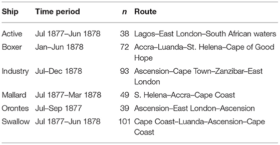
Table 2. Log books digitized for the period 1877/78: ship name, time period covered, number of noon observations assimilated, and route.

Upper air data for the 1926/27 case were taken from Stickler et al. (2014a,b). They include 500 hPa geopotential height data from aircraft ascents at Soesterberg/De Bilt in the Netherlands and Lindenberg in Germany. Furthermore, I analyzed pilot balloon winds at 1.5 and 5.5 km which were compared with wind at 850 and 500 hPa in 20CRv3. In few cases with several ascents on the same day (typically morning and afternoon), the two ascents were averaged. Note that the wind data were not assimilated but only used for evaluation. An overview is given in Table 3.

TABLE 3

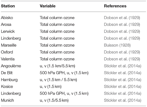
Table 3. Total column ozone and upper-air series used for the assimilation experiments 1926/27.

Finally, total column ozone data were taken from the early European network of Dobson et al. (1929), complemented by data from Marseille (Buisson, 1928). The data were digitized by us previously (Brönnimann et al., 2003) and are available from the World Ozone and Ultraviolet Radiation Data Center (WOUDC; see also Staehelin et al., 1998, for the Arosa record). The data are available only as daily means, but ozone observations are best performed with low solar zenith angle, so daily means in Europe will not differ much from 12 UTC. The column ozone series used are summarized in Table 3.

Processing of Observations

Prior to assimilation, all observations were debiased relative to 20CRv3. Temperature, geopotential height, and total column ozone observations were debiased by fitting the first two harmonics of the seasonal cycle to both, observations and 20CRv3, and then subtracting the difference. Differences in the seasonal cycles can be due to observation biases (radiation errors), due to model shortcomings, or they can be true (e.g., due to local effects). For pressure data, which have no strong seasonal cycle, only the difference in the mean values was corrected. For the ship pressure data in 1877–1878, differences between ship data and 20CR were calculated for each ship and then corrected by subtracting the average deviation per ship. This debiasing minimizes the effects of systematic differences. It should however be noted that this preserves the 20CRv3 annual cycle and the seasonal mean spatial patterns, while the assimilated observations add intra-seasonal variability in time and space.

Offline Data Assimilation Method

For all following analyses, I used the Ensemble Square Root filter (Whitaker and Hamill, 2002) to assimilate historical observations y into 20CRv3 (x_b) off-line (the model was not rerun), yielding x_a.

First the ensemble mean is updated and then anomalies from the mean:

$\begin{array}{llll}\overline{{\text{x}}_{\text{a}}}& =& \overline{{\text{x}}_{\text{b}}}+\text{K}(\overline{\text{y}}-\text{H}\overline{{\text{x}}_{\text{b}}})& (1)\end{array}$

$\begin{array}{ll}{x^{\prime }}_a={x^{\prime }}_b+\tilde{K}\left(y^{\prime }-H{x^{\prime }}_b\right)=\left(I-\tilde{K}H\right){x^{\prime }}_b,\text{with:}{y}^{\prime }=0& (2)\end{array}$

H is the Jacobian matrix of the linear observation operator that extracts total column ozone from the model state. The Kalman gain matrix K for the ensemble mean and the anomalies from the mean is defined as:

$\begin{array}{llll}\text{K}& =& {\text{P}}^{\text{b}}{\text{H}}^{\text{T}}{\left(\text{H}{\text{P}}^{\text{b}}{\text{H}}^{\text{T}}+\text{R}\right)}^{-1}& (3)\end{array}$

$\begin{array}{llll}\tilde{\text{K}}& =& {\text{P}}^{\text{b}}{\text{H}}^{\text{T}}{\left[{\left(\sqrt{\text{H}{\text{P}}^{\text{b}}{\text{H}}^{\text{T}}+\text{R}}\right)}^{-1}\right]}^{\text{T}}\times {\left(\sqrt{\text{H}{\text{P}}^{\text{b}}{\text{H}}^{\text{T}}+\text{R}}+\sqrt{\text{R}}\right)}^{-1}& (4)\end{array}$

P^b and R are the background error and observation error covariance matrices, respectively. The former is calculated from the 80 members; no localization was performed. The latter is assumed diagonal which makes it possible to assimilate observations sequentially.

An important parameter to set in a reanalysis concerns the observation error R, which measures the error of the term y–Hx (i.e., it also accounts for the error in the representation of the observation in the model). For the assimilation of temperature (which is less well-represented by the model than pressure), I assume an error of 3² K². For sea-level pressure I used an error of 3² hPa², which accounts for the numerous error sources related to historical pressure measurements and their processing (Brugnara et al., 2015). For total column ozone I assumed an error variance of 15² DU² (this is derived from previous work with historical data, see Brönnimann et al., 2003), for 500 hPa geopotential height I assume an error of 35² gpm², consistent with estimates in Wartenburger et al. (2013). Note that in all cases, part of the systematic error is removed beforehand in a debiasing step. Before assimilation, observations were checked against the background and were only assimilated if y–Hx was smaller than 3 × (HP^bH^T + R)^0.5.

Experiments and Evaluation

For each case, several experiments were performed. For the case of 1807, experiments were performed in which only pressure observations, only temperature observations, or both were assimilated. Similarly, for the 1877, case experiments assimilating only ship-based pressure data or assimilating also land station data are performed. For the 1926/7 case I assimilated total column ozone or 500 hPa GPH. Each of these experiments was not only run in a full mode (i.e., all obaservations are assimilated, termed FULL), but also in a leave-one-out mode (LOO, all observations except one are assimilated, and the analysis is then evaluated at that location). Table 4 lists all experiments.

TABLE 4

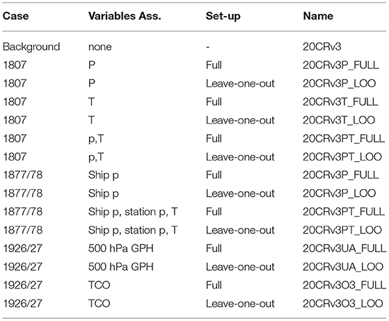
Table 4. Assimilation experiments performed in this study.

The results are compared to the observations described in the earlier section. Independent data are available for all case studies, and the results from the LOO experiments are also independent. Comparison (in FULL) of the analysis with the assimilated series will obviously produce good results, which therefore are clearly marked on the figure. However, it is still important to address, e.g., the reduction of the ensemble spread in FULL. When calculating the skill measures, I excluded days in which no observations were assimilated (and, obviously, days in which evaluation observations were missing).

All experiments are analyzed with respect to the same three diagnostics: the Pearson correlation, the root mean squared error (RMSE) and the ensemble standard deviation. The former two diagnostics are calculated after subtracting the mean annual cycle (in this case also for station pressure) by fitting the first two harmonics, as described for the pre-processing of observations. In the evaluation I always calculate the same diagnostics for the background (20CRv3 without assimilation) and the experiment (Table 4), and then results are either plotted for both or only their ratio. For the correlation at a given station, the change is often small compared to changes between stations and therefore hard to visualize with one color scale. I therefore also defined a “scaled improvement” as (r_EPX-r_BCK)/(1-r_BCK), where r_EPX is the correlation between the observations and the experiment under questions and r_BCK is the correlation between observations and the background (i.e., 20CRv3 before assimilation). This serves as a “magnification” of the correlation change (but, conversely, when using the same color scale across all stations this is quickly saturated if the change is large).

In the interpretation of results, it is important to keep in mind that the assimilation is off-line. The results are therefore pessimistic in the sense that an improvement is not communicated to the next time step. The potential improvement of cycling the analysis might be much larger. However, this set-up allows the assessment of observational input in a common framework. The results are optimistic in the sense that biases are subtracted beforehand. Current reanalysis system often use online bias correction schemes, which however may not work as well as our ex-post bias subtraction.

Results

Data Coverage for the 1780s

Before presenting the results of the assimilation experiments, I analyzed existing inventories of surface observations with respect to the question how far back a reanalysis could possibly be extended. 20CRv3 reaches back to 1806, although with extremely sparse input in the first 30 years or so. A backward extension seems possible because, when going further back in time, the number of observations increases (Brönnimann et al., 2019). This is because in the politically troubled times of the coalition Wars, the number of observations in Europe decreased. Decades earlier, during the peak of the Enlightenment, the number of observations had reached a temporary peak.

A potential coverage map of the 1780s is shown in Figure 1 (based on Kington, 1988; Brönnimann et al., 2019; Winkler, 2020). In this decade, the Societas Meteorologica Palatina ran its famous network (Pappert et al., 2021). At the same time, the French medical society had a dense network, as did the Bavarian Academy (Winkler, 2020). In Italy, astronomer Giuseppe Toaldo organized a network. Data are also available from outside Europe from the colonial world. The Moravian Brethren measured in Labrador (Demarée and Ogilvie, 2008), the Caribbean is relatively well-covered with observations, and data are also available for outposts in Asia, Africa, and South America (Brönnimann et al., 2019). Even the first measurements from Australia fall into this decade (Gergis et al., 2009). Note, however, that this map shows all measurements known to be taken; some may not be found, or may be of low quality. Some of the series have only short segments of measurements, others cover the entire decade. Note also that this map does not show marine data, which are particularly important, but are extremely sparse in the 1780s.

FIGURE 1

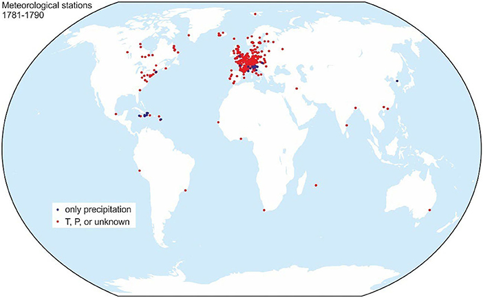
Figure 1. Global map of meteorological stations in the decade 1781–1790, irrespective of whether the data are digitally available, imaged, or whether the location of the hard copies is even known.

From this map it seems that an extension of reanalyses backward to the 1780s seems possible. Kington (1988) has produced hand-analyzed maps for this decade, and Pappert et al. (2022) have produced daily pressure and temperature maps for the winter 1788/89 based on an analog approach, augmented with an offline Ensemble Kalman Filter. Since sufficient observations were available for these two approaches, there could also be sufficient observations for a dynamical reanalysis. When going even further back in time the number of observations drops. It reaches the same number as in 1806 (when 20CRv3 starts) in the early 1770s (Brönnimann et al., 2019). However, there are almost no marine data in the 1770s (much less than in 1806) and therefore an extension beyond ca. 1781 might prove difficult.

Assimilating Additional Station Data

In order to address the value of additional measurements, I take the example of 1807. This is one of the first years to be included in the extended version of 20CRv3, which is based on only eight pressure series over Europe. At the same time, this is an interesting year as Europe experienced an extremely warm and dry summer (Casty et al., 2005) and, although during a period with few climate observations, it is relatively straight forward to find additional series. In this study I add 30 series (detailed in Table 1), the distribution of the stations selected is shown in Figure 2.

FIGURE 2

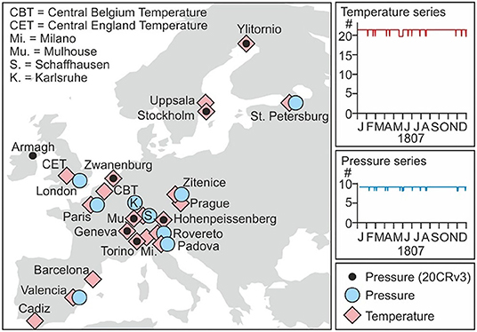
Figure 2. Map of daily time series used in the experiments of the year 1807. Black dots indicate the pressure series already assimilated into 20CRv3. The colored symbols indicate stations assimilated in this article. Time series indicate the number of assimilated series per variable.

First, I assimilated only pressure information. Results are shown in Figure 3 (top row). The LOO experiment confirms that assimilating additional pressure series leads to an improvement of SLP at the left-out locations. However, as evidenced in FULL, the assimilation of pressure worsens the skill for temperature (lower correlation, higher RMSE) at a majority of the locations, particularly those in Central Europe, although only by a small amount.

FIGURE 3

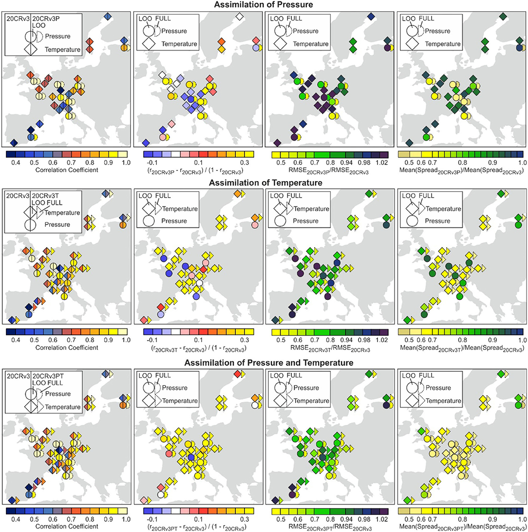
Figure 3. Results of the experiments for 1807 for correlation, scaled improvement (saturated >0.3 as these cases are visible in the correlation directly), ratio of RMSE, and ratio of ensemble spread. Dashed outlines indicate results from the FULL assimilation that are not independent, solid outlines are based on independent data (data retained for evaluation or LOO approach). Note that some of the color-scales are not equidistant.

In the second experiments I assimilated only temperature data (Figure 3, middle row). Similar as for pressure, the LOO experiment shows increasing skill for temperature at left-out locations. This increase is relatively large. The FULL model, conversely, shows a decrease of the skill for many pressure series (mostly those in Western Europe), but again only by a small amount. The assimilation of both, pressure and temperature, shows an increase in LOO for both variables at all locations. The FULL model obviously well reproduces all variables; the ensemble spread is reduced by ca. 50%.

More Marine Data Input

In the second case I tested whether assimilating more marine pressure data could help to improve historical reanalyses. The case selected for this covers July 1877 to June 1878, when during a strong El Niño event, droughts were observed globally (Singh et al., 2018). Data from six ships were assimilated; a map of the ship tracks is shown in Figure 4. The tracks cover mainly the South Atlantic, but many also continue into the Indian Ocean (or vice versa). Note that the ship data are sparse and also land data are sparse, such that we have only around 6 observations on any single day (compared to 30 observations in 1807 over a much smaller region). This must be considered when analyzing the leave-one-out results. Typically there is only a handful of measurements for a given day, over a region that is much larger than Europe in the 1807 case.

FIGURE 4

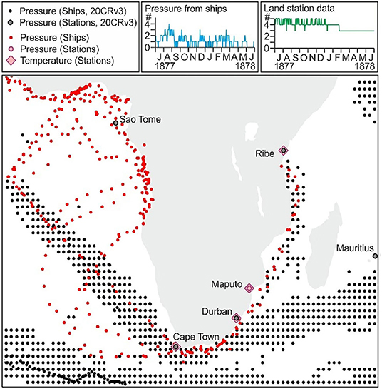
Figure 4. Map of daily time series used in the experiments of the year 1807. Black dots (ships) and circles (stations) indicate the pressure series already assimilated into 20CRv3. The colored symbols indicate stations assimilated in this article. The lines indicate the numbers of ship and land station data assimilated per day.

As for 1807, I performed LOO and FULL models, both for experiments with only ship pressure data or with both ship data and land-based data. For the evaluation, all ship data were pooled. Results (Figure 5) show that assimilating ship pressure has only a very small influence on the other ship data in the LOO approach, and also the effect on land stations is small. In fact, we do not see a change when analyzing correlation directly, only when plotting the scaled improvement. However, the effect is positive (increase of correlation, decrease of RMSE, decrease of spread) for all cases.

FIGURE 5

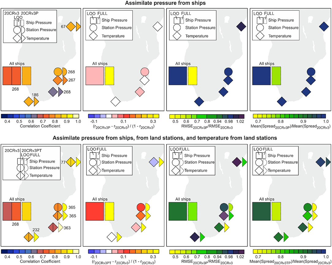
Figure 5. Results for 1877/78 for correlation, scaled improvement, ratio of RMSE, and ratio of ensemble spread. Top: Assimilating only ship pressure, bottom: assimilating ship pressure as well as land station data. The numbers in the left panels indicate the observation pairs used for each correlation. Dashed outlines indicate results from the FULL assimilation that are not independent, solid outlines are based on independent data (data retained for evaluation or LOO approach). Note that the color-scale for the RMSE ratio is not equidistant.

When assimilating both ship and land data, results are similar. The improvement is generally stronger and is now also seen when plotting correlation directly, but we also find cases (one in correlation, one in RMSE) in which skill measures decrease in the LOO experiment. The FULL model shows high correlations (mostly above 0.9), a reduction of the RMSE by 20–50% and a reduction of the ensemble spread by 20–30%. Overall, significant improvement could thus be reached over Subsaharan Africa and the South Atlantic, which is notable as further ship logbooks are available that could be digitized for this extremely important climate event.

Upper-Air Input

The third case analyzed concerns the period October 1927 to September 1927. The period was chosen because a rather dense network of total column ozone instruments was operating in Europe. In addition, also upper-air data are available for this time. Table 3 lists the data used for this case, Figure 6 shows a map of the stations. In contrast to the 1807 case, note that series have many and long gaps and therefore the number of available observations varies significantly. Again, FULL and LOO experiments were carried for the case of assimilating 500 hPa geopotential height and for the case of assimilating total column ozone. Apart from LOO experiments, independent evaluation is also possible in the respective other variable (I did not perform a combined experiment) and with the help of upper-level wind data, which were not assimilated. It should be noted, however, that these upper-level wind measurements presumably have large errors.

FIGURE 6

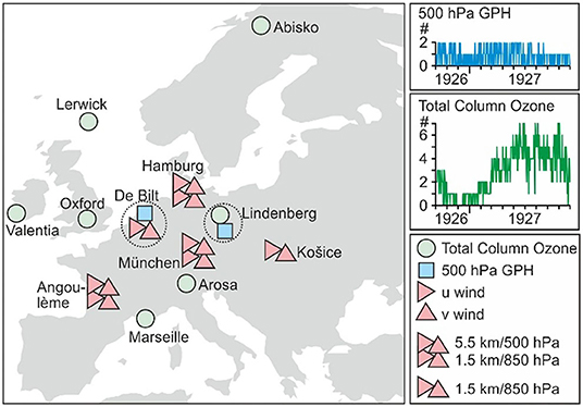
Figure 6. Map with predictors used in the 1926/27 experiment. Time series indicate the number of observations assimilated per day.

Only two series of 500 hPa GPH were assimilated (De Bilt, Lindenberg). The LOO experiment (Figure 7, upper row) shows an improvement for both stations. As for the 1877 case, the correlation difference is so small that it cannot by visualized when plotting only the correlation directly (left), but only by the scaled improvement. The corresponding plots clearly show improvement not only for 500 hPa height, but (in FULL) also for total column ozone. Correlation increases at all seven sites. Correlations also mostly increase for wind at 5.5 km, but we see no improvement for wind at 1.5 km (see Table 3 for station information).

FIGURE 7

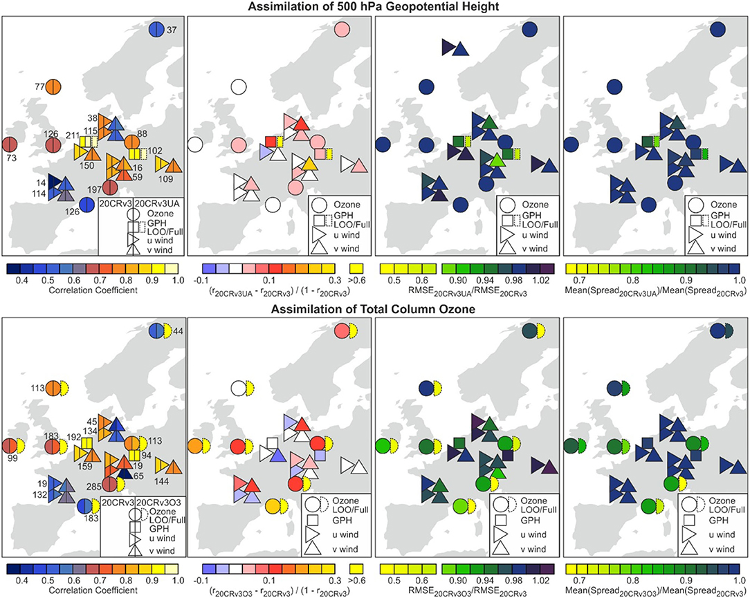
Figure 7. Results of the 1926/27 experiment for correlation, scaled improvement, ratio of RMSE, and ratio of ensemble spread for the assimilation of 500 hPa geopotential height (top) and total column ozone (bottom). The numbers in the left panels indicate the observation pairs used for each correlation. Dashed outlines indicate results from the FULL assimilation that are not independent, solid outlines are based on independent data (data retained for evaluation or LOO approach).

The reduction of RMSE follows the results for the correlations. It is mostly on the order of a few percent. The reduction of the ensemble spread lies in a similar range. Thus, while the assimilation of 500 hPa clearly improves the result, the improvement is modest (note, however, that I only assimilate two records). That said, it should again be noted that the updated fields are not cycled back to the model.

Total Column Ozone Input

In the second set of experiments, I assimilated total column ozone. 20CRv3 includes total column ozone as a prognostic variable determined from a gas-phase parameterization of ozone production and loss (McCormack et al., 2006). This variable was added to our state vector x (Equations 1–4). We evaluated it against 500 hPa height, upper-level wind, and (in the LOO set-up) total column ozone (Figure 7, lower row). In the LOO set-up, the assimilation of total column ozone clearly improves ozone at the neighboring stations. An improvement is also generally found for wind at 5.5 km, while wind at 1.5 km shows no improvement. For 500 hPa, no improvement is found, however, it should be noted that correlation is already very high (above 0.9 in anomalies); this distinguishes this case from the previous cases.

Discussion

Observations Assimilated

In all cases analyzed, additional observations generally led to an improvement of the results. This may seem trivial, but is not. In fact, in the case of 1807, assimilating additional pressure data slightly decreased the skill of temperature and vice versa, which could indicate that the background error covariance matrix does not adequately represent co-variances in observations. However, this decrease in skill is relatively small, and assimilating both variables leads to increased skill everywhere.

In the case of 1807, the increase in skill when assimilating both pressure and temperature is relatively pronounced, which is expected as, on the one hand, 20CRv3 is not well-constrained and, on the other hand, a large amount of additional information is assimilated (note that 20CRv3 does not assimilate temperature). For the case of 1877 over Africa, 20CRv3 also is not well-constrained. The data assimilated are extremely sparse, but still lead to a large-scale, albeit small improvement of the assimilation. In contrast, in the 1926/27 case 20CRv3 is already extremely well-constrained only from the surface, with anomaly correlation exceeding 0.9 for 500 hPa GPH observations (this in itself is surprising given even just the errors in the observations). Presumably, 20CRv3 is better than the evaluation data and perhaps even better than the assimilated data. It is thus much more difficult to improve this situation than to improve fields in 1877/78 over Africa. Total column ozone and 500 hPa GPH both lead to an improvement, as seen in the corresponding other variable, in a leave-one-out approach, and in independent upper-level wind data.

The improvement in the case of 1926/27 is not very large, but well visible in the middle troposphere and tropopause (i.e., column ozone). No improvement is found in the lower troposphere. This could arguably be very different if the assimilated fields were cycled, which is a limitation of this sutdy. In fact, assimilating upper-air data led to an improvement in a historical reanalysis as demonstrated by the ERA-PreSAT experimental product (Hersbach et al., 2017), which assimilated upper-air data starting in 1939. It should also be noted that the assimilation set up used in this study is deliberately simple in that no localization was used.

In our approach, observations were debiased with respect to 20CRv3 and therefore did not introduce unwanted biases. This is an idealized set-up, which mimics what an online-bias correction could do in an optimal case. It is well-known that in a more realistic set-up, changes in observing system are one possible cause of biases and step changes in historical reanalysis data sets (e.g., Bloomfield et al., 2018; Cid et al., 2018; Blanc et al., 2021 and many more), even in the satellite era (e.g., Grant et al., 2008). Hence much more work arguably needs to be done to be able to assimilate additional variables. When assimilating remote, historical data in a period of sparse observations, quality control is difficult and the danger of introducing biases exists (see also Dee et al., 2014), which is not analyzed in this study. Remaining outliers also could destroy the skill in experiments as those shown in this article. Conversely, it should be noted that historical reanalyses provide a tool for the quality control, outlier screening or even break detection in observations.

The results from this study show that historical observations can indeed help to improve reanalyses. Many of the historical observations are already available in digital form, such as the upper-air information (Stickler et al., 2014a,b; Haimberger, 2021). In other cases additional data rescue efforts are required. The simple experiments presented in this article can help to prioritize future data rescue efforts.

Finally, experiments such as those presented here can possibly be used as a “poor-man's assimilation” to generate post-processed fields, e.g., for case studies. As the analyses are not cycled back to the model, they may not be physically consistent in a strict sense. However, as this study shows, resulting fields might be statistically improved and may be useful for further applications. In particular, such approaches may make use of additional variables such as temperature, which are difficult to assimilate in a conventional reanalysis, but in the setting used here (in particular the debiasing) can provide useful additional information.

Boundary Conditions and Forcing Data

An additional way in which observations support historical reanalysis is in the form of model boundary condition or forcing data. Although this article does not analyse their potential in terms of improvements that could be reached in this way, some aspects should be briefly listed for the sake of completeness. For atmospheric reanalyses, sea-surface temperature and sea ice are arguably the most important boundary condition. Especially when going further back in time, sea-surface temperature are sparse, and existing data sets still have issues (Chan et al., 2019) that affect reanalyses generated from them. Work is ongoing to further improve (and better quantify uncertainties of) the sea-surface temperature record (Kennedy et al., 2019). Any information on sea ice could be particularly beneficial. For coupled simulations, sea-surface salinity data could contribute important information (Reverdin and Friedman, 2018), as could snow data for the land surface (see Brönnimann et al., 2018b for an overview). Potential skill could also arise from constraining a reanalysis in the tropical stratosphere using a reconstruction of the Quasi-Biennial Oscillation (Brönnimann et al., 2007).

Observations could also help to improve external forcings applied to the models. As an example, Figure 8 shows transmission in the visible and near-infrared derived from spectrobolometric measurements performed by the Smithsonian Institution (Stickler et al., 2014a) at Mount Wilson, California (1905–1920). The data clearly show the eruption of Novarupta in Alaska in 1912. Although the data from the Smithsonian Institution have informed reconstructions of volcanic aerosol optical depth, the spectral transmission data could provide much more detailed and more specific information on aerosol-radiation interaction.

FIGURE 8

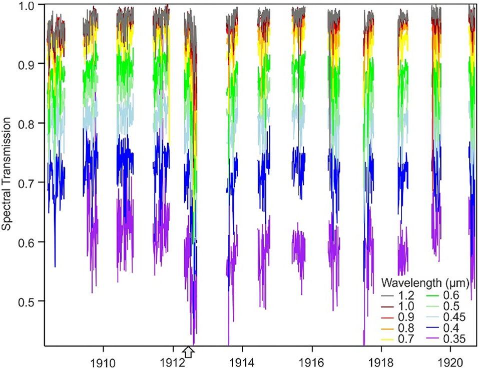
Figure 8. Daily spectral transmission at Mount Wilson from the observations of the Smithsonian institution (Stickler et al., 2010). The arrow marks the eruption of Novarupta in Alaska.

Conclusions

This article addresses the question how additional observations could improve historical reanalyses. Using an off-line Ensemble Kalman Filter approach, I assimilated observations into Version 3 of the “Twentieth Century Reanalysis” (20CRv3) for distinct historical cases. In addition to surface or sea-level pressure, I also assimilated temperature, upper-air data, and column ozone. For a very early case (Europe in 1807), the additional observations led to a substantial improvement, although assimilating more pressure data alone did not increase the skill for temperature and vice versa. For Africa in 1877/78, during a strong El Niño event, a small positive effect of assimilating additional ship data could be found across the entire domain despite that fact that observations are very sparse and only a handful of measurements per day could be assimilated. Finally, for the case of 1926/27, it could be shown that assimilating upper air data or even total column ozone data improves the fields in the middle troposphere and the tropopause level, while 20CRv3 is already extremely well-constrained in the lower troposphere such that no improvement could be found.

Finally, I addressed the question how much further back reanalyses could be extended if all observations taken were available in digital form and of sufficient quality. I estimate that land-based information would support a dynamical reanalysis back to around 1781, although there is very little information from ships for this time. Further data rescue efforts would however be needed for such an extension. For certain analyses such as case studies, post-processed 20CRv3 fields generated with a similar approach as used in this study could prove beneficial.

Data Availability Statement

Historical observations and the assimilation code are available in the electronic supplement (Data Sheet 1). 20CRv3 reanalysis data (ensemble members) are available from NCAR/UCAR (https://rda.ucar.edu/datasets/ds131.3/). Smithsonian Institution measurements are available on the electronic supplement (Data Sheet 2).

Author Contributions

SB conceived and conducted the research and wrote the paper.

Funding

This work was supported by Swiss National Science Foundation project WeaR (188701), the European Commission (ERC Grant PALAEO-RA, 787574), the Federal Office of Meteorology and Climatology MeteoSwiss in the framework of GCOS Switzerland (project Long Swiss Meteorological Series), and the Newton Fund/WCSSP Project Improve the marine observations coverage across southern Africa and Climate Data Rescue Service of C3S, contract C3S_DC3S311a_Lot1.

Conflict of Interest

The author declares that the research was conducted in the absence of any commercial or financial relationships that could be construed as a potential conflict of interest.

Publisher's Note

All claims expressed in this article are solely those of the authors and do not necessarily represent those of their affiliated organizations, or those of the publisher, the editors and the reviewers. Any product that may be evaluated in this article, or claim that may be made by its manufacturer, is not guaranteed or endorsed by the publisher.

Acknowledgments

I like to thank Rob Allan and the ACRE initiative as well as Stefan Grab for sharing historical observations from 1877/78, Yuri Brugnara for station data in 1807 and Chesley McColl Peter Stucki for their help in downloading and processing 20CRv3 ensemble members.

Supplementary Material

The Supplementary Material for this article can be found online at: https://www.frontiersin.org/articles/10.3389/fclim.2022.880473/full#supplementary-material

References

Allan, R., Brohan, P., Compo, G. P., Stone, R., Luterbacher, J., and Brönnimann, S. (2011). The international Atmospheric Circulation Reconstructions over the Earth (ACRE) initiative. Bull. Amer. Meteorol. Soc. 92, 1421–1425. doi: 10.1175/2011BAMS3218.1

CrossRef Full Text | Google Scholar

Auchmann, R., Brönnimann, S., Breda, L., Bühler, M., Spadin, R., and Stickler, A. (2012). Extreme climate, not extreme weather: the summer of 1816 in Geneva, Switzerland. Clim. Past 8, 325–335. doi: 10.5194/cp-8-325-2012

CrossRef Full Text | Google Scholar

Barriendos, M., Martín-Vide, J., Peña, J. C., and Rodríguez, R. (2002). Daily meteorological observations in Cádiz_San Fernando. Analysis of the documentary sources and the instrumental data content (1786–1996). Clim. Change 53, 151–170. doi: 10.1023/A:1014991430122

CrossRef Full Text | Google Scholar

Bergström, H., and Moberg, A. (2002). Daily air temperature and pressure series for Uppsala (1722–1998). Clim. Change 53, 213–252. doi: 10.1023/A:1014983229213

CrossRef Full Text | Google Scholar

Blanc, A., Blanchet, J., and Creutin, J.-D. (2021). Past evolution and recent changes in Western Europe large-scale circulation. Weather Clim. Dynam. 3, 231–250. doi: 10.5194/wcd-2021-69

CrossRef Full Text | Google Scholar

Bloomfield, H. C., Shaffrey, L. C., Hodges, K. I., and Vidale, P. L. (2018). A critical assessment of the long-term changes in the wintertime surface Arctic Oscillation and Northern Hemisphere storminess in the ERA20C reanalysis. Environ. Res. Lett. 13:094004. doi: 10.1088/1748-9326/aad5c5

CrossRef Full Text | Google Scholar

Brázdil, R. L., Řezníčková, H., Valá,šek, H., and Kotyza, O. (2007). Early instrumental meteorological observations in the Czech lands. Part III. Frantisek Jindrich Jakub Kreybich, Zitenice, 1787-1829. Meteorologický časopis 10, 63–74.

Google Scholar

Brönnimann, S., Allan, R., Ashcroft, L., Baer, S., Barriendos, M., Brázdil, R., et al. (2019). Unlocking pre-1850 instrumental meteorological records: a global inventory. Bull. Amer. Meteorol. Soc. 100, ES389–ES413. doi: 10.1175/BAMS-D-19-0040.1

CrossRef Full Text | Google Scholar

Brönnimann, S., Allan, R., Atkinson, C., Buizza, R., Bulygina, O., Dahlgren, P., et al. (2018b). Observations for reanalyses. Bull. Amer. Meteorol. Soc. 99, 1851–1866. doi: 10.1175/BAMS-D-17-0229.1

CrossRef Full Text | Google Scholar

Brönnimann, S., Annis, J. L., Vogler, C., and Jones, P. D. (2007). Reconstructing the Quasi-Biennial Oscillation back to the early 1900s. Geophys. Res. Lett. 34:L22805. doi: 10.1029/2007GL031354

CrossRef Full Text | Google Scholar

Brönnimann, S., Brugnara, Y., Allan, R. J., Brohan, P., Brunet, M., Compo, G. P., et al. (2018a). A roadmap to climate data rescue services. Geosci. Data J. 5, 28–39. doi: 10.1002/gdj3.56

CrossRef Full Text | Google Scholar

Brönnimann, S., Staehelin, J., Farmer, S. F. G., Cain, J. C., Svendby, T. M., and Svenøe, T. (2003). Total ozone observations prior to the IGY. I: a history. Q. J. Roy. Meteorol. Soc. 129B, 2797–2817. doi: 10.1256/qj.02.118

CrossRef Full Text | Google Scholar

Brugnara, Y., Auchmann, R., Brönnimann, S., Allan, R. J., Auer, I., Barriendos, M., et al. (2015). A collection of sub-daily pressure and temperature observations for the early instrumental period with a focus on the “year without a summer” 1816. Clim. Past 11, 1027–1047. doi: 10.5194/cp-11-1027-2015

CrossRef Full Text | Google Scholar

Brugnara, Y., Auchmann, R., Brönnimann, S., Bozzo, A., Berro, D. C., and Mercalli, L. (2016). Trends of mean and extreme temperature indices since 1874 at low-elevation sites in the Southern Alps. J. Geophys. Res. 121, 3304–3325. doi: 10.1002/2015JD024582

CrossRef Full Text | Google Scholar

Brugnara, Y., Pfister, L., Villiger, L., Rohr, C., Isotta, F. A., and Brönnimann, S. (2020). Early instrumental meteorological observations in Switzerland: 1708–1873. Earth Syst. Sci. Data 12, 1179–1190. doi: 10.5194/essd-12-1179-2020

CrossRef Full Text | Google Scholar

Buisson, H. (1928). Mesures de l'ozone de la haute atmosphère pendant l'année 1927. C. R. Acad. Sci. 186, 1229–1230.

Google Scholar

Casty, C., Wanner, H., Luterbacher, J., Esper, J., and Böhm, R. (2005). Temperature and precipitation variability in the European Alps since 1500. Int. J. Climatol. 25, 1855–1880. doi: 10.1002/joc.1216

CrossRef Full Text | Google Scholar

Chan, D., Kent, E. C., Berry, C. I., and Huybers, P. (2019). Correcting datasets leads to more homogeneous early-twentieth-century sea surface warming. Nature 571, 393–397. doi: 10.1038/s41586-019-1349-2

PubMed Abstract | CrossRef Full Text | Google Scholar

Cid, A., Wahl, T., Chambers, D. P., and Muis, S. (2018). Storm surge reconstruction and return water level estimation in Southeast Asia for the 20th century. J. Geophys. Res. 123, 437–451. doi: 10.1002/2017JC013143

CrossRef Full Text | Google Scholar

Compo, G. P., Slivinski, L. C., Whitaker, J. S., Sardeshmukh, P. D., McColl, C., Brohan, P., et al. (2019). The International Surface Pressure Databank version 4. Research Data Archive at the National Center for Atmospheric Research, Computational and Information Systems Laboratory.

Google Scholar

Compo, G. P., Whitaker, J. S., and Sardeshmukh, P. D. (2006). Feasibility of a 100-year reanalysis using only surface pressure data. Bull. Amer. Meteorol. Soc. 87, 175–190. doi: 10.1175/BAMS-87-2-175

CrossRef Full Text | Google Scholar

Compo, G. P., Whitaker, J. S., Sardeshmukh, P. D., Matsui, N., Allan, R. J., Yin, X., et al. (2011). The twentieth century reanalysis project. Q. J. Roy. Meteorol. Soc. 137, 1–28. doi: 10.1002/qj.776

CrossRef Full Text | Google Scholar

Cornes, R. C., Jones, P. D., Briffa, K. R., and Osborn, T. J. (2012a). A daily series of mean sea-level pressure for London, 1692-2007. Int. J. Climatol. 32, 641–656. doi: 10.1002/joc.2301

CrossRef Full Text | Google Scholar

Cornes, R. C., Jones, P. D., Briffa, K. R., and Osborn, T. J. (2012b). A daily series of mean sea-level pressure for Paris, 1670-2007. Int. J. Climatol. 32, 1135–1150. doi: 10.1002/joc.2349

CrossRef Full Text | Google Scholar

Dee, D. P., Balmaseda, M, Balsamo, G, Engelen, R., Simmons, A. J., and Thépaut, J.-N. (2014). Toward a consistent reanalysis of the climate system. BAMS 95, 1235–1248. doi: 10.1175/BAMS-D-13-00043.1

CrossRef Full Text | Google Scholar

Demarée, G. R., and Ogilvie, A. E. J. (2008). The Moravian missionaries at the Labrador coast and their centuries-long contribution to instrumental meteorological observations. Clim. Change 91, 423–450. doi: 10.1007/s10584-008-9420-2

CrossRef Full Text | Google Scholar

Demarée, R. R., Lachaert, P.-J., Verhoeve, T., and Thoen, E. (2002). “The Long-Term Daily Central Belgium Temperature (CBT) Series (1767–1998) and Early Instrumental Meteorological Observations in Belgium,” in D. Camuffo and P. Jones, editors. Improved Understanding of Past Climatic Variability from Early Daily European Instrumental Sources (Springer, Dordrecht). 269–293.doi: 10.1007/978-94-010-0371-1_10

CrossRef Full Text | Google Scholar

Di Napoli, G., and Mercalli, L. (2008). Il clima di Torino: tre secoli di osservazioni meteorologiche. SMS, Turin.

Google Scholar

Dobson, G. M. B., Harrison, D. N., and Lawrence, J. (1929), Measurements of the amount of ozone in the Earth's atmosphere its relation to other geophysical conditions, Part III. Proc. Phys. Soc. London A122, 456–486. doi: 10.1098/rspa.1929.0034

CrossRef Full Text | Google Scholar

Domínguez-Castro, F., Vaquero, J., Rodrigo, F., Farrona, A., Gallego, M., García-Herrera, R., et al. (2014). Early Spanish meteorological records (1780_1850). Int. J. Climatol. 34, 593–603. doi: 10.1002/joc.3709

CrossRef Full Text | Google Scholar

Gergis, J., Karoly, D. J., and Allan, R. J. (2009). A climate reconstruction of Sydney Cove, New South Wales, using weather journal and documentary data, 1788-1791. Aust. Meteorol. Oceanogr. J. 58, 83–98. doi: 10.22499/2.5802.001

CrossRef Full Text | Google Scholar

Grant, A., Brönnimann, S., and Haimberger, L. (2008). Recent Arctic warming vertical structure contested. Nature 455, E2–E3. doi: 10.1038/nature07257

PubMed Abstract | CrossRef Full Text | Google Scholar

Haimberger, L. (2021). Service C3S C311c Support for Climate Reanalysis Including Satellite Data Rescue Lot 2: Historic Upper-Air Data. Available online at: https://img.univie.ac.at/forschung/meteorologie/projekte/copernicus/

Google Scholar

Hersbach, H., Brönnimann, S., Haimberger, L., Mayer, M., Villiger, L., Comeaux, J., et al. (2017). The potential value of early (1939–1967) upper-air data in atmospheric climate reanalysis. Q. J. Roy. Meteorol. Soc. 143, 1197–1210. doi: 10.1002/qj.3040

CrossRef Full Text | Google Scholar

Jones, P. D., and Lister, D. H. (2002). The daily temperature record for St. Petersburg (1743–1996). Clim. Change 53, 253–267, doi: 10.1007/978-94-010-0371-1_9

CrossRef Full Text | Google Scholar

Kennedy, J. J., Rayner, N. A., Atkinson, C. P., and Killick, R. E. (2019). An ensemble data set of sea-surface temperature change from 1850: the Met Office Hadley Centre HadSST.4.0.0.0 data set. J. Geophys. Res. 124, 7719–7763. doi: 10.1029/2018JD029867

CrossRef Full Text | Google Scholar

Kington, J. A. (1988). The Weather of the 1780s Over Europe. Cambridge: Cambridge University Press.

Google Scholar

Klingbjer, P., and Moberg, A. (2003). A composite monthly temperature record from Tornedalen in northern Sweden, 1802_2002. Int. J. Climatol. 23, 1465–1494. doi: 10.1002/joc.946

CrossRef Full Text | Google Scholar

Laloyaux, P., de Boisseson, E., Balmaseda, M., Bidlot, J.-R., Brönnimann, S., Buizza, R., et al. (2018). CERA-20C: A coupled reanalysis of the Twentieth Century. J. Adv. Model. Earth Syst. 10, 1172–1195. doi: 10.1029/2018MS001273

CrossRef Full Text | Google Scholar

Maugeri, M., Buffoni, L., and Chlistovsky, F. (2002a). Daily Milan temperature and pressure series (1763-1998): history of the observations and data and metadata recovery. Clim. Change 53, 101–117. doi: 10.1007/978-94-010-0371-1_4

CrossRef Full Text | Google Scholar

Maugeri, M., Buffoni, L., Delmonte, B., and Fassina, A. (2002b). Daily Milan temperature and pressure series (1763-1998): completing and homogenising the data. Clim. Change 53, 119–149. doi: 10.1007/978-94-010-0371-1_5

CrossRef Full Text | Google Scholar

McCormack, J. P., Eckermann, S. D., Siskind, D. E., and McGee, T. J. (2006). CHEM2D-OPP: a new linearized gas-phase ozone photochemistry parameterization for high-altitude NWP and climate models. Atmos. Chem. Phys 6, 4943–4972 doi: 10.5194/acp-6-4943-2006

CrossRef Full Text | Google Scholar

Moberg, A., Bergström, H., Krigsman, J. R., and Svanered, O. (2002). Daily air temperature and pressure series for Stockholm (1756-1998). Clim. Change 53, 171–212. doi: 10.1023/A:1014966724670

CrossRef Full Text | Google Scholar

Noone, S., Atkinson, C., Berry, D. I., Duun, R. J. H., Freeman, E., Perez Gonzalez, I., et al. (2021). Progress towards a holistic land and marine surface meteorological database and a call for additional contributions. Geosci. Data J. 8, 103–120. doi: 10.1002/gdj3.109

CrossRef Full Text | Google Scholar

Pappert, D., Barriendos, M., Brugnara,1, Y., Imfeld, N., Jourdain, S., Przybylak, R., et al. (2022). Statistical reconstruction of daily temperature and sea-level pressure in Europe for the severe winter 1788/9. Clim. Past Discuss. [preprint]. doi: 10.5194/cp-2022-10 in review.

CrossRef Full Text | Google Scholar

Pappert, D., Brugnara, Y., Jourdain, S., Pospieszyńska, A., Przybylak, R., Rohr, C., et al. (2021). Unlocking weather observations from the Societas Meteorologica Palatina (1781–1792). Clim. Past 17, 2361–2379 doi: 10.5194/cp-17-2361-2021

CrossRef Full Text | Google Scholar

Parker, D. E., Legg, T. P., and Folland, C. K. (1992). A new daily Central England temperature series, 1772–1991. Int. J. Clim. 12, 317–342. doi: 10.1002/joc.3370120402

PubMed Abstract | CrossRef Full Text | Google Scholar

Poli, P., Hersbach, H., Dee, D. P., Berrisford, P., Simmons, A. J., Vitart, F., et al. (2018). ERA-20C: an atmospheric reanalysis of the Twentieth Century. J. Clim. 29, 4083–4097. doi: 10.1175/JCLI-D-15-0556.1

CrossRef Full Text | Google Scholar

Reverdin, G., and Friedman, A. R. (2018). Bin-averaged SSS in the Atlantic Ocean.

Google Scholar

Rodríguez, R., Barriendos, M., Jones, P., Martín-Vide, J., and Pena, J. (2001). Long pressure series for Barcelona (Spain). Daily reconstruction and monthly homogenization. Int. J. Climatol. 21, 1693–1704. doi: 10.1002/joc.696

CrossRef Full Text | Google Scholar

Singh, D., Seager, R., Cook, B. I., Cane, M., Ting, M., Cook, E., et al. (2018). Climate and the global famine of 1876–78. J. Clim. 31, 945–9467. doi: 10.1175/JCLI-D-18-0159.1

CrossRef Full Text | Google Scholar

Slivinski, L. C., Compo, G. P., Sardeshmukh, P. D., Whitaker, J. S., McColl, C. M., Allan, R., et al. (2020). An evaluation of the performance of the 20th Century Reanalysis version 3. J. Clim. 34, 1417–1438. doi: 10.1175/jcli-d-20-0505.1

CrossRef Full Text | Google Scholar

Slivinski, L. C., Compo, G. P., Whitaker, J. S., Sardeshmukh, P. D., Giese, B., McColl, C., et al. (2019). Towards a more reliable historical reanalysis: improvements to the Twentieth Century Reanalysis system. Q. J. Roy. Meteorol. Soc. 145, 2876–2908. doi: 10.1002/qj.3598

CrossRef Full Text | Google Scholar

Staehelin, J., Renaud, A., Bader, J., McPeters, R., Viatte, P., Hoegger, B., et al. (1998). Total ozone series at Arosa (Switzerland): homogenisation and data comparison. J. Geophys. Res. 103, 5827–5841. doi: 10.1029/97JD02402

CrossRef Full Text | Google Scholar

Stepanek, P. (2005). Air Temperature Fluctuations in the Czech Republic in the Period of Instrumental Measurements. PhD thesis, Masaryk University, Brno, Czech Republic.

Google Scholar

Stickler, A., Brönnimann, S., Jourdain, S., Roucaute, E., Sterin, A., Nikolaev, D., et al. (2014a). Description of the ERA-CLIM historical upper-air data. Earth Syst. Sci. Data 6, 29–48. doi: 10.5194/essd-6-29-2014

CrossRef Full Text | Google Scholar

Stickler, A., Brönnimann, S., Valente, M. A., Bethke, J., Sterin, A., Jourdain, S., et al. (2014b). ERA-CLIM: historical surface and upper-air data for future reanalyses. Bull. Amer. Meteorol. Soc. 95, 1419–1430 doi: 10.1175/BAMS-D-13-00147.1

CrossRef Full Text | Google Scholar

Stickler, A., Grant, A. N., Ewen, T., Ross, T. F., Vose, R. S., and Comeaux, J. (2010) The comprehensive historical upper-air network. Bull. Amer. Meteorol. Soc. 91, 741–751. doi: 10.1175/2009BAMS2852.1

CrossRef Full Text | Google Scholar

Thorne, P. W., Allan, R. J., Ashcroft, L., Brohan, P., Dunn, R. J. H., Menne, M. J., et al. (2017). Towards an integrated set of surface meteorological observations for climate science and applications. Bull. Amer. Meteorol. Soc. 98, 2689–2702. doi: 10.1175/BAMS-D-16-0165.1

CrossRef Full Text | Google Scholar

Wartenburger, R., Brönnimann, S., and Stickler, A. (2013). Observation errors and representativity errors in upper-air observations. J. Geophys. Res. 118, 12012–12028. doi: 10.1002/2013JD020156

CrossRef Full Text | Google Scholar

Whitaker, J. S., and Hamill, T. M. (2002). Ensemble data assimilation without perturbed observations. Mon. Weather Rev. 130, 1913–1924. doi: 10.1175/1520-0493(2002)130andlt;1913:EDAWPOandgt;2.0.CO;2

PubMed Abstract | CrossRef Full Text | Google Scholar

Winkler, P. (2006). Hohenpeissenberg 1781-2006 - das älteste Bergobservatorium der Welt. Deutscher Wetterdienst, Offenbach am Main.

Google Scholar

Winkler, P. (2020). Geschichte der Meteorologie in Bayern bis zum Jahr 1900. Geschichte der Meteorologie in Deutschland, Offenbach, DWD.

Google Scholar