Verification Data and the Skill of Decadal Predictions

The utility of a forecast depends on its skill as demonstrated by past performance. For most forecasts errors rapidly become large compared to uncertainties in the observation-based state of the system and, for this reason, it is usually deemed adequate to assess predictions against a single verification dataset. Eleven reanalyses and station-based analyses of annual mean surface air temperature are compared as are basic skill measures obtained when using them to verify decadal prediction hindcasts from the Canadian Centre for Climate Modelling and Analysis forecasting system. There are differences between reanalysis and station-based analyses which translate also into differences in basic skill scores. In an average sense, using station-based verification data results in somewhat better correlation skill. The spread between the locally best and worst scores is obtained for individual forecast ensemble members and for ensemble mean forecasts compared to individual analyses. The comparison of ensemble mean forecasts against different analyses can result in apparent skill differences, and using a “favorable” analysis for verification can improve apparent forecast skill. These differences may be more pertinent for longer time averages and should be considered when verifying decadal predictions and when comparing the skill of decadal prediction systems as part of a model intercomparison project. Either a particular analysis could be recommended by the decadal prediction community, if such could be agreed on, or the ensemble average of a subset of recent analyses could be used, assuming that ensemble averaging will act to average out errors.

1. Introduction

Current weather and climate predictions ranging from hours to decades are usually based on ensembles of model-based forecasts. Verifying the skill of the forecasts has always been a critical but non-trivial task. The implicit assumption is that the error in a forecast is so much larger than the error of the verifying analysis that the latter does not appreciably contaminate the skill measure. A forecast can take various forms which, in the most straightforward case, is a deterministic forecast of a variable such as temperature at a particular time in the future. As the forecast range passes beyond the range for which an instantaneous deterministic forecast is appropriate, the forecast typically becomes that of a time average of the quantity.

Decadal prediction, alternatively near-term climate prediction, refers to the prediction of the climate system on timescales of a year to one (or more) decades. The predictions may be generated by statistical methods based on the past behavior of the climate system but are most frequently made with coupled climate models (Kirtman et al., 2013; Kushnir et al., 2019). For a model-based prediction an observation-based estimate of the state of the climate system serves to initialize the model. The model is integrated forward in time with specified external forcings (e.g., greenhouse gas concentrations, solar, and volcanic variations) to generate the forecast. The initial conditions are an attempt to specify the state of the climate system but will not be everywhere exact. This uncertainty in initial conditions implies uncertainty in the subsequent predictions and forecast systems typically probe this uncertainty by performing multiple integrations with slightly differing initial conditions. The resulting “cone” of forecasts is a representation of this uncertainty. Forecast results may be characterized statistically in terms of probability measures or deterministically by averaging the forecasts and providing quantitative values.

A decadal prediction experiment is part of the fifth Coupled Model Intercomparison Project (CMIP5, Taylor et al., 2012) and is a prominent component (Boer et al., 2016) of the current sixth version of this activity (CMIP6, Eyring et al., 2016). The World Climate Research Programme (WCRP) Grand Challenge on near-term climate prediction encourages research into decadal prediction with the goal of fostering applications (e.g., Kushnir et al., 2019). Decadal prediction largely concentrates on predicting the basic variables of temperature and precipitation. On annual and multi-annual timescales the predicted variables are typically the anomalies from climatology of annual and/or multi-annual means (e.g., Boer et al., 2013; Smith et al., 2013). The WMO Lead Centre for Annual-to-Decadal Climate Prediction (https://hadleyserver.metoffice.gov.uk/wmolc/) “collects and provides hindcasts, forecasts and verification data from a number of Global Producing Centres and other Contributing Centres worldwide” and provides useful links concerning decadal prediction. The “Global Annual to Decadal Climate Update,” available from the WMO website, provides decadal predictions of basic variables and of a range of climatically important indices (Hermanson et al., 2022).

Predictions must be accompanied by measures of skill in order to be credible and useful, particularly for real-world applications. Assessing skill is a technical matter (e.g., Jolliffe and Stephenson, 2012; Goddard et al., 2013; Sospedra-Alfonso and Boer, 2020) that aims to quantify the match between predictions and verifying data over a sequence of forecasts. The prediction data is based on retrospective forecasts (or hindcasts) of past cases. For statistical stability it is important that the hindcast sequence be as long as possible. Correlation, mean square error and mean square skill score are basic skill measures which, although not without fault, are straightforward, familiar, and commonly used.

The information used to initialize coupled forecasting models and to verify the forecasts are often based on reanalyses. The “Reanalyses.org Home Page” at (https://reanalyses.org/) is one locus of information on reanalyses. As noted there, a reanalysis combines observations (from many sources) with a numerical model that simulates one or more aspects of the Earth system to generate a synthesized estimate of the state of the system. Results are typically available on global grids several times a day and climate values are obtained by averaging. Despite being observation-based, the results from different systems are not identical since reanalysis methods and their implementation, as well as the observations on which the reanalyses are based, are not uniform across time and analysis systems. Just as climate model simulation and prediction results are intercompared in CMIP, reanalyses are now being intercompared for similar reasons. As well as Reanalyses.org, the SPARC Reanalysis Intercomparison Project (S-RIP at https://s-rip.ees.hokudai.ac.jp/) provides information and links. Fujiwara et al. (2017) give an introduction to S-RIP and an overview of the analysis systems considered. Martineau et al. (2018) produce a zonal-mean data set on pressure levels to facilitate reanalysis intercomparison.

Station-based climate analyses are an alternative source of verification data for decadal predictions of basic variables like temperature and precipitation. The approach in this case is to provide gridded products derived from quality controlled station data of the variables.

The statistics relating reanalyses, station-based analyses, and forecasts depend on the averaging period considered. The kinds of local structures that are dominant for short range forecasts are averaged out when longer time scales are considered. The consequences of using different sources of verifying data to calculate prediction skill for longer time averages is not immediately obvious and this is investigated here for forecasts of annual mean temperature. Annual means are basic to decadal climate prediction and surface air temperature and precipitation are basic physical variables that have direct application for climate services (WMO, 2016). We concentrate on temperature since it is considered to be both better observed and better forecast than precipitation.

It is expected that model-based predictions will differ more from observation-based verifying analyses than the analyses will differ among themselves. Nevertheless, differences in analyses can have consequences for the assessment of decadal prediction skill (e.g., Boer et al., 2019a). We quantify these differences for decadal predictions of annual mean temperature made with the latest version of the Canadian Centre for Climate Modelling and Analysis (CCCma) decadal forecasting system (Sospedra-Alfonso et al., 2021).

2. Data

The observation-based surface air temperature data used in this analysis were made available on a latitude longitude grid as an outgrowth of the SPARC Reanalysis Intercomparison Protect (S-RIP) (Fujiwara et al., 2017; Martineau et al., 2018). A subset of seven of the reanalyses systems listed in those papers is considered here as indicated in Table 1. Corresponding station-based data also listed in Table 1 are obtained from the indicated sources. These and the reanalyses data total eleven observation-based products that are examined in what follows.

TABLE 1

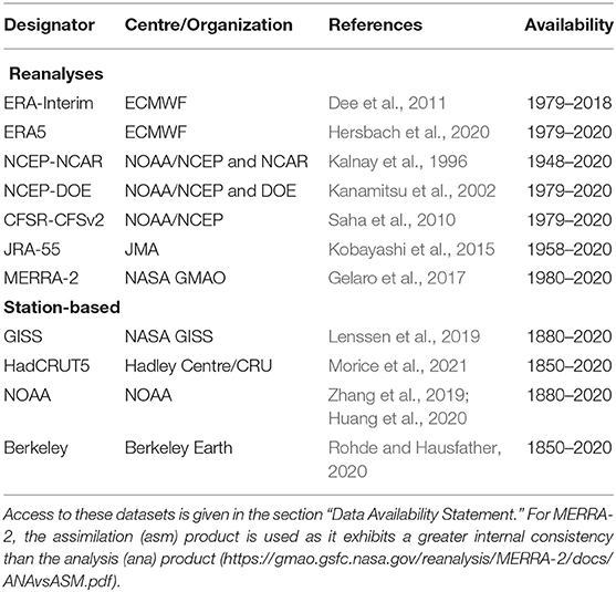
Table 1. Reanalyses and station-based surface air temperature data.

The forecast data used are from the CCCma decadal forecasting system's participation in the Decadal Climate Prediction Project's (DCPP, Boer et al., 2016) contribution to CMIP6. The 40-member forecast ensemble is produced with version 5 of the Canadian Earth System Model (CanESM5) which is integrated for ten years from realistic initial conditions once a year from 1961 to the present using prescribed external forcing (Sospedra-Alfonso and Boer, 2020; Sospedra-Alfonso et al., 2021).

The analysis data are represented as X_k = X_k(λ, φ, t) and are functions of longitude, latitude and time where k denotes the data sets listed in Table 1. In the face of differing lengths of record across the analyses, a common intercomparison period consisting of the 39 years from 1980 to 2018 is used. The corresponding forecast data from CCCma hindcasts is represented as Y_k = Y_k(λ, φ, t) where here the subscript denotes the ensemble member of the forecast. There are 40 ensemble members for each forecast and 11 sources of verifying data.

The CCCma decadal forecasts and the observation-based data are regridded to a common 2.5° resolution. Second order climate statistics involve anomalies from the time mean and these are taken as the basic variables in what follows. We treat both an ensemble of forecasts and an ensemble of observations.

The X_k and Y_k are anomalies from their time means so average to zero over the analysis period. Since the quantities are functions of time, space, and ensemble number, the statistics considered depend on combinations of spatial, temporal and ensemble averaging. Ensemble averaging is indicated by subscript “A” or curly brackets, i.e., X_A = {X_k}. All quantities are understood to be functions of time, unless time averaged, and functions of the ensemble index unless ensemble averaged. The analyses can be represented in various ways as

$\begin{array}{ll}{X}_k=X_A+X_k^{*}={\alpha }_{k}t+X_k^{\prime }={\alpha }_{A}t+X_k^{″}={\alpha }_{A}t+{\alpha }_k^{*}t+X_k^{\prime }& (1)\end{array}$

where deviations from the ensemble mean are indicated by an asterisk. In (1), α_kt is the linear trend fitted to X_k, $X_k^{\prime }$ the variation about that trend, α_At the ensemble mean trend, $X_k^{″}$ the variation about the ensemble mean trend, and ${\alpha }_k^{*}t$ the deviation of the individual trend from the ensemble mean trend.

3. Globally Averaged Annual Mean Temperature

Let X_k in (1) represent the globally averaged annual mean temperature anomaly. Figure 1A displays the evolution of X_k for the different analyses together with the ensemble mean X_A and the ensemble mean linear trend α_At for the 1980–2018 period. While the overall features are the same in all analyses, as would be expected, there are also differences in detail. The deviations $X_k^{*}$ of the individual analyses from the ensemble mean X_A are plotted in Figure 1B.

FIGURE 1

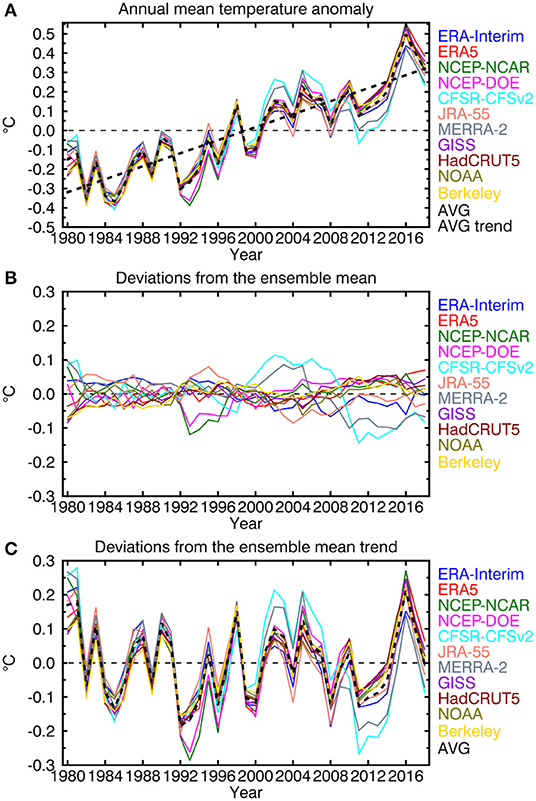
Figure 1. Globally averaged observation-based (A) anomalies of annual mean temperature X_k from the 1980 to 2018 average; (B) deviations $X_k^{*}=X_k-X_A$ of individual analyses from the ensemble mean X_A; and (C) deviations $X_k^{″}=X_k-{\alpha }_{A}t$ around the ensemble mean linear trend. The thick dashed curves in the top and bottom panels correspond to the ensemble average X_A and the thick black dashed line in the top panel is the ensemble mean linear trend α_At for the period.

The increase in globally averaged annual mean temperature is a notable feature of Figure 1A. Individual linear trends α_k are a simple metric of this and are plotted in Figure 2A together with the ensemble mean trend α_A. Reanalysis results are in black and station-based results in gray. The station-based trends are all above the average while the reanalysis-based trends vary about the ensemble mean.

FIGURE 2

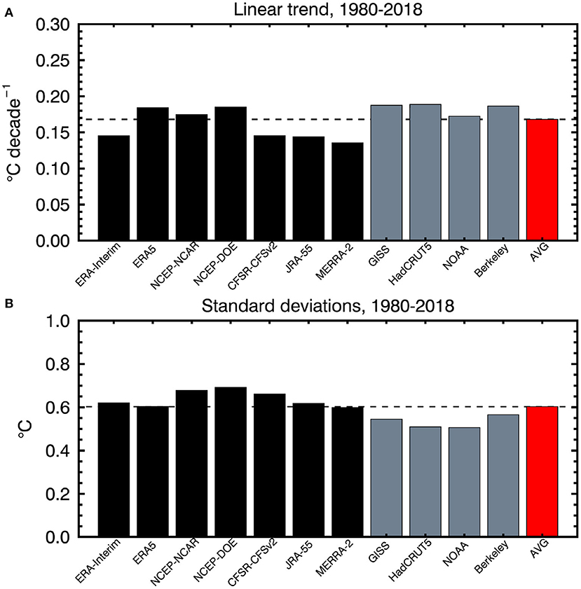
Figure 2. (A) Linear trends α_k and (B) standard deviations $\sqrt{\langle {\sigma }_{X_k}^2\rangle }$ of globally averaged annual mean temperature from the reanalyses (black) and station-based analyses (gray). The red bar is (A) the trend α_A of the ensemble mean and (B) the standard deviation $\sqrt{\langle \left\{{\sigma }_{X_k}^2\right\}\rangle }$ of the ensemble average of the variances.

Figure 1C displays the variations $X_k^{″}$ about the ensemble mean trend. To the extent that the linear trend is an indication of the forced component, it could presumably be estimated from simulation results. In a simulation, internally generated variability about the forced trend would be present but, in the absence of initialization, the variations would not be expected to coincide with those observed so would detract from skill rather than contribute to it. $X_k^{″}$ serves as a rough indication of the kind of natural variations, superimposed on externally forced GHG warming, that might be predicted with suitable models and observation-based initial conditions.

Under time averaging (indicated by an overbar) and ensemble averaging (indicated by curly brackets or the subscript A) the overall variance of annual mean temperature has the components

$\begin{array}{ll}\begin{array}{l}\left\{\overline{X_k^2}\right\}=\overline{X_A^2}+\left\{\overline{X_k^{*2}}\right\}\hfill \\ ={\alpha }_A^2{\sigma }_t^2+\left\{\overline{X_k^{″2}}\right\}\hfill \\ =\left\{{\alpha }_k^2\right\}{\sigma }_t^2+\left\{\overline{X_k^{\prime 2}}\right\}\hfill \\ ={\alpha }_A^2{\sigma }_t^2+\left\{{\alpha }_k^{*2}\right\}{\sigma }_t^2+\left\{\overline{X_k^{\prime 2}}\right\}\hfill \end{array}& (2)\end{array}$

represented as

$\begin{array}{ll}\begin{array}{c}{\sigma }_X^2={\sigma }_{X_A}^2+{\sigma }_{X^{*}}^2={\sigma }_{{\alpha }_{A}t}^2+{\sigma }_{X^{"}}^2={\sigma }_{\alpha t}^2+{\sigma }_{X^{\prime }}^2={\sigma }_{{\alpha }_{A}t}^2+{\sigma }_{{\alpha }^{*}t}^2+{\sigma }_{X^{\prime }}^2\end{array}& (3)\end{array}$

The fractional contributions to the overall variance of the different components are

$\begin{array}{ll}\begin{array}{l}1=\frac{{\sigma }_{X_A}^2}{{\sigma }_X^2}+\frac{{\sigma }_{X^{*}}^2}{{\sigma }_X^2}=0.97+0.03\hfill \\ =\frac{{\sigma }_{{\alpha }_{A}t}^2}{{\sigma }_X^2}+\frac{{\sigma }_{X″}^2}{{\sigma }_X^2}=0.74+0.26\hfill \\ =\frac{{\sigma }_{\alpha t}^2}{{\sigma }_X^2}+\frac{{\sigma }_{X^{\prime }}^2}{{\sigma }_X^2}=0.75+0.25\hfill \\ =\frac{{\sigma }_{{\alpha }_{A}t}^2}{{\sigma }_X^2}+\frac{{\sigma }_{{\alpha }^{*}t}^2}{{\sigma }_X^2}+\frac{{\sigma }_{X^{\prime }}^2}{{\sigma }_X^2}=0.74+0.01+0.25\hfill \end{array}& (4)\end{array}$

Taken together, the analyses of globally averaged annual mean temperature anomalies for the 1980–2018 period have about 97% of their variance in common. For this globally averaged variable, some 74% of the variance is accounted for by the ensemble mean linear trend and 26% by the variation about it. This is similar to the variance accounted for by the ensemble mean of the linear trends fitted to the individual analyses at just over 75% with just about 25% of the variance associated with variations about the means. The ensemble variance of the trend itself is small at about 1%. Obviously, and as expected, the analyses agree to a large extent among themselves although for globally averaged annual mean temperature much of the variance is associated with a comparatively strong linear trend.

4. The Geographical Distribution of the Variance of Annual Mean Temperature

Forecast results are compared to analysis data in terms of temporal anomalies. The standard skill measures of correlation and mean square error are based on the variances and covariances of the anomalies.

4.1. Overall Variance Levels

For X_k now representing the anomalies of local annual mean temperature (rather than of the global mean temperature) the temporal variance of the analyses is $\langle {\sigma }_{X_k}^2\rangle =\langle \overline{X_k^2}\rangle$ where angular brackets indicate the global average. Figure 2B plots the square roots of these quantities together with the square root of the ensemble mean $<\left\{{\sigma }_{X_k}^2\right\}>$. The variances of the reanalyses values are larger than or near to that of the mean while the station-based variances are smaller.

Component variances following (2) are calculated locally at each grid point and then globally averaged. The fractional contributions to the overall variance following (4) are

$\begin{array}{l}1=\frac{<{\sigma }_{X_A}^2>}{<{\sigma }_X^2>}+\frac{<{\sigma }_{X^{*}}^2>}{<{\sigma }_X^2>}=0.83+0.17\hfill \\ =\frac{<{\sigma }_{\alpha t}^2>}{<{\sigma }_X^2>}+\frac{<{\sigma }_{X^{\prime }}^2>}{<{\sigma }_X^2>}=0.24+0.76\hfill \end{array}$

In this case, some 83% of the overall variance is common to the analyses with about 17% differing across analyses. The local trends account for about 24% of the variance with 76% associated with the variation about these trends. These numbers contrast with the values for globally averaged annual mean temperature since the global averaging reduces the overall variance and enhances the fraction that is common to the analyses.

4.2. Geographical Distribution of Variances

From (2,3), the geographical distribution of the overall variance is

$\begin{array}{l}{\sigma }_X^2=\left\{\overline{X_k^2}\right\}=\overline{X_A^2}+\left\{\overline{X_k^{*2}}\right\}={\sigma }_{X_A}^2+{\sigma }_{X^{*}}^2\end{array}$

with the associated standard deviations σ_X and ${\sigma }_{X^{*}}$ plotted in the upper panels of Figure 3. The bottom panel plots the ratio ${\sigma }_{X^{*}}^2/{\sigma }_X^2$ giving the fraction of the overall variance that is associated with differences across analyses. The complementary term ${\sigma }_{X_A}^2/{\sigma }_X^2=1-{\sigma }_{X^{*}}^2/{\sigma }_X^2$ is the fraction of variance common to the analyses.

FIGURE 3

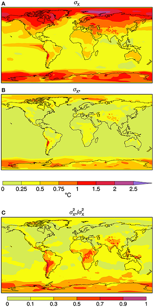
Figure 3. Standard deviations (A) σ_X and (B) ${\sigma }_{X^{*}}$ of annual mean temperature under time and ensemble averaging where ${\sigma }_X^2=\left\{\overline{X_k^2}\right\}=\overline{X_A^2}+\left\{\overline{X_k^{*2}}\right\}={\sigma }_{X_A}^2+{\sigma }_{X^{*}}^2$ following (2,3) together with the (C) ratio ${\sigma }_{X^{*}}^2/{\sigma }_X^2$ giving the fraction of the overall variance accounted for by differences among analyses.

The geographical distribution of variability represented by σ_X has the expected distribution with larger values tending to occur at high latitudes and/or over land and weaker variability over the oceans excepting the eastern tropical Pacific. The variability associated with differences in analyses ${\sigma }_{X^{*}}$ has comparatively large values over high elevation areas and at southern high latitudes. By contrast with σ_X, values of ${\sigma }_{X^{*}}$ are comparatively small over the northern ocean and also over land areas, except for the polar regions.

The ratio ${\sigma }_{X^{*}}^2/{\sigma }_X^2$ is a measure of the differences across analyses. It has a marked geographical distribution with a distinct gradient from lower values in the northern hemisphere to larger values in the southern hemisphere. For the green areas in the plot, the ratio is <10% and these areas account for most of the northern hemispheric land and ocean, although with some areas having values within 10–30%. Values are broadly larger in the southern hemisphere, especially over tropical land and in polar regions. These results are, perhaps, a bit surprising since temperature is one of the best observed variables, especially since the satellite era.

The analyses have much of their variance in common. Differences between pairs of variances are tested following Pitman (1939) using the t-statistic in the form

$\begin{array}{ll}t=\frac{(F-1)\sqrt{n-2}}{2\sqrt{F(1-r^2)}}& (5)\end{array}$

where F is the usual F-ratio and n is the number of years, in this case 39. The test takes into account that the variances have a common component via the correlation term. The test nominally determines if the variance that is not common to the two analyses is statistically significant, i.e., not due only to sampling error. The number of pairs with different variances, based on this test, is plotted in Figure 4.

FIGURE 4

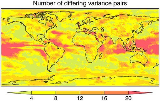
Figure 4. The number of pairs of variances that differ among the 11 analyses at the 95% confidence level according to the Pitman (1939) test which discounts the common variance.

Areas with fewer differences are found mainly over the extratropical oceans while areas with the most disagreement are found over tropical oceans, at least according to this test. These latter regions are also regions of weak variability. The pattern of Figure 4 is not particularly similar to that of the bottom panel of Figure 3 for ${\sigma }_{X^{*}}^2/{\sigma }_X^2$ at least over tropical land and Antarctic regions. The overall implication of Figures 3, 4 is that the geographical pattern of the variance of annual mean temperature can differ non-trivially from analysis to analysis and from place to place.

4.3. Linear Trend

The linear trend is a simple measure of the increase in annual mean temperature over the period considered. From (2,3), the variances associated with local trend and non-trend variability are

$\begin{array}{c}{\sigma }_X^2=\left\{\overline{X_k^2}\right\}=\left\{{\alpha }_k^2\right\}{\sigma }_t^2+\left\{\overline{X_k^{\prime 2}}\right\}={\sigma }_{\alpha t}^2+{\sigma }_{X^{\prime }}^2\end{array}$

The geographic distribution of the trend that is common to the analyses is characterized by the ensemble mean trend α_A which is plotted in the upper panel of Figure 5. The fraction of the local variance associated with linear trend ${\sigma }_{\alpha t}^2/{\sigma }_X^2$ is plotted in the lower panel of Figure 5.

FIGURE 5

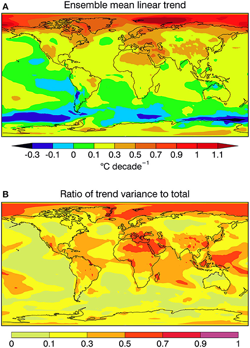
Figure 5. (A) Ensemble mean linear trend α_A and (B) the local ratio ${\sigma }_{{\alpha }_t}^2/{\sigma }_X^2$ of the trend variance to the total variance.

Despite the increase in globally averaged temperature seen in Figure 5A, there are notable local regions of negative temperature trend in Figure 5 for this climatological period (1980–2018) as seen also for instance in Hartmann et al. (2013, Fig 2.22) for the period 1981–2012. Nevertheless, as expected, temperature trends are generally positive, most notably over land, and especially so at higher northern latitudes.

The fraction of the variance accounted for by the trend in Figure 5 conforms broadly to the strength of the trend itself in northern regions of positive trends while this is less the case in southern regions of weak or negative trends. The relative importance of the trend would be expected to be larger in regions of weak variability compared to regions of strong interannual variability. The skill of a prediction will be expected to depend on the comparative magnitude of the trends in the forecasts and in the verifying data.

5. Skill Measures

Differences in verification data will result in differences in skill, but are the differences large enough to be of interest, particularly for the more heavily averaged quantities considered in decadal prediction? The consequences for basic skill measures due to differences in verifying analyses are investigated by using them to verify the results of a CCCma decadal prediction experiment. Annual mean temperature is considered since it is a basic decadal prediction variable as well as the variable with the best current skill. Bigger discrepancies very likely exist for other variables, such at precipitation, but this is not pursued here.

Current approaches typically compare ensemble mean forecasts to a single verifying data set, but we may compare the ensemble mean forecast to the ensemble mean of the analyses, individual analyses to the ensemble mean forecast and individual ensemble members to individual analyses. The three cases are

$\begin{array}{lll}{r}_{AA}& =& \frac{\overline{X_A{Y}_A}}{{\sigma }_{X_A}{\sigma }_{Y_A}}\\ r_{kA}& =& \frac{\overline{X_k{Y}_A}}{{\sigma }_{X_k}{\sigma }_{Y_A}}\\ r_{kl}& =& \frac{\overline{X_k{Y}_l}}{{\sigma }_{X_k}{\sigma }_{Y_l}}& (6)\end{array}$

Here r_AA is the correlation of the ensemble mean forecast with the ensemble mean of the analyses, r_kA the correlation of the ensemble mean forecast with the k individual analyses to illustrate the consequence of differences in verifying data sets on skill, and r_kl the scatter that is possible if a single forecast is compared to a single set of verifying data. Here k = 1…11 for the 11 analyses and l = 1…40 for the 40 ensemble members of the forecasts.

Taking the forecasts and analyses as vectors, standard deviation measures the length of the vectors, correlation the angle between them and root means square error the distance between them. While correlation is independent of a simple scaling of the forecast variance or length, mean square error (MSE) is not. The MSE values paralleling (6) are

$\begin{array}{lll}{e}_{AA}^2& =& \overline{{(Y_A-X_A)}^2}={\sigma }_{X_A}^2+{\sigma }_{Y_A}^2-2{\sigma }_{X_A}{\sigma }_{Y_A}{r}_{AA}\\ e_{kA}^2& =& \overline{{(Y_A-X_k)}^2}={\sigma }_{X_k}^2+{\sigma }_{Y_A}^2-2{\sigma }_{X_k}{\sigma }_{Y_A}{r}_{kA}\\ e_{kl}^2& =& \overline{{(Y_l-X_k)}^2}={\sigma }_{X_k}^2+{\sigma }_{Y_l}^2-2{\sigma }_{X_k}{\sigma }_Y{r}_{kl}& (7)\end{array}$

Differences in results illustrate the consequences of taking all of the information into account (in the sense of the ensemble means), a single analysis for the verification of the ensemble mean forecast, and a single forecast compared to a single analysis.

There are 11 analyses, 40 ensemble members, and forecasts from 1 to 10 years for a possible 4,400 plots of r_kl. This reduces to 110 plots for r_kA and to 10 for r_AA. In what follows forecasts for the first 5 years are considered since the skill of annual mean temperature plateaus by that time. This reduces the potential number of plots by half but plotting the 55 values for r_kA, let alone the 2,200 values for r_kl is unwieldy. Dimensionality is reduced by considering globally averaged values < r_kA >, forecasts for years 1, 3, and 5 for r_AA, and the locally best and worst values of r_kA and r_kl.

6. Correlation Skill

The three versions of correlation skill in (6) give an indication of the kinds of results that can arise based on individual and/or averaged forecasts and analyses.

6.1. Skill of Ensemble Mean Forecasts and Verifying Data

Current approaches typically compare ensemble mean forecasts to a single verifying data set. When multiple verifying data sets are available it is natural to consider their ensemble mean also. The implicit assumption is that each analysis is composed of information on the actual state of the system plus unavoidable analysis errors arising from problems with the raw data as well as difficulties associated with the particular analysis system.

The forecast and analysis ensembles are, of course, different in kind as well as in size. The forecast ensemble may be thought of as being composed of predictable (or signal) and unpredictable (or noise) components Y_l = ψ + y_l (e.g., Boer et al., 2013, 2019a,b) where the predictable component ψ is common to the ensemble members while the unpredictable noise component y_l differs across the ensemble. Together they represent a range of realizations of the evolution of the forecasting system arising from differences in initial conditions nominally close to the actual initial state of the system and representing the uncertainty in the initial state. By contrast, the analysis ensemble represents a particular evolution of the physical system plus error expressed as X_k = X + ϵ_k where X is the actual value and ϵ_k the error in the kth analysis system. The physical system will also have predictable and unpredictable components here represented as X = χ + x so that X_k = χ + x + ϵ_k. The ensembles behave differently under ensemble averaging. For the forecasts, Y_A = ψ + y_A → ψ with the arrow indicating the large ensemble limit where the unpredictable or noise component is averaged out and only the predictable or signal component remains. For the analysis ensemble X_A = X + ϵ_A = χ + x + ϵ_A where ϵ_A becomes small in the large ensemble limit only if there are no appreciable systematic analysis errors due to data or other difficulties. Ensemble averaging acts to reduce unpredictable variance in the forecasts but not in the analysis ensemble although it is expected to reduce the error variance.

The correlation r_AA between the ensemble mean forecasts Y_A and the ensemble mean of the analyses X_A is plotted in Figure 6 for annual average temperature for year 1, 3, and 5 forecasts. The results are largely similar to those from the analysis of an earlier version of the forecasting system (Boer et al., 2013), except for the loss of skill in the North Atlantic subpolar region discussed by Sospedra-Alfonso et al. (2021).

FIGURE 6

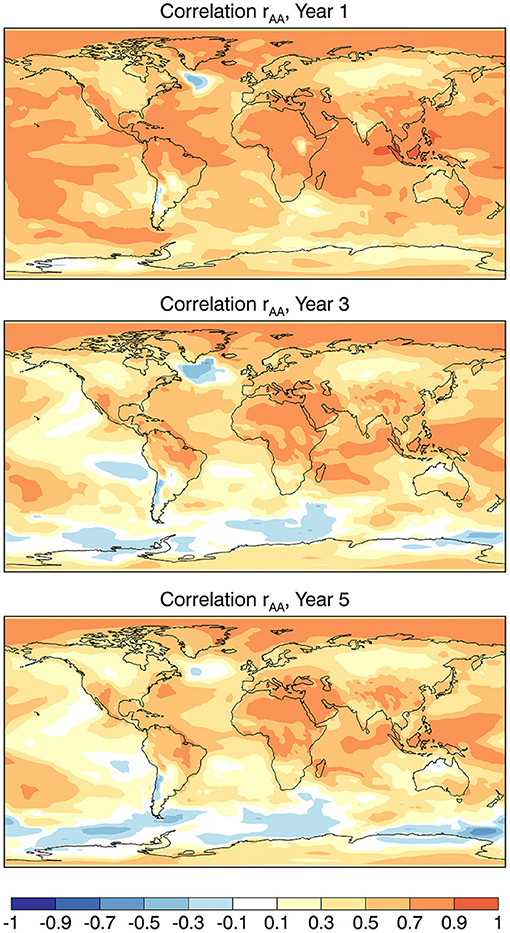
Figure 6. Correlation skill r_AA between the ensemble mean forecast and ensemble mean analysis.

6.2. The Skill of the Ensemble Mean Forecast

Current approaches typically compare the ensemble mean forecast Y_A against a single verifying data set X. The availability of several analyses X_k provides some information of the consequences of different verifying analyses for the correlation skill of annual mean temperature. Figure 7 plots the global average < r_kA > for the first 5 years of the forecasts. The correlations decline until about year 4 and then remain approximately the same. This kind of result is seen in Boer et al. (2013, 2019a) and is consistent with the initial decline in the skill of the initialized internally generated component until the more or less constant correlation skill of the externally forced (e.g., due to GHGs, land use change) component takes over. The perhaps surprising aspect is that, even for this heavily averaged quantity, there is a noticeable difference in the calculated skill of the forecast depending on the verification used. The best correlations are with HadCRUT5 which is also the analysis that has the strongest trend (0.19°C/decade) in Figure 2A. The lowest correlation values are associated with JRA-55 and ERA-Interim, which are among the three analyses with the lowest trends (0.14 and 0.15°C/decade, respectively) in Figure 2A.

FIGURE 7

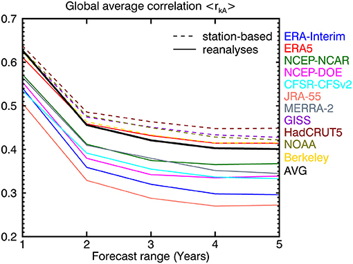
Figure 7. The global average of the correlation < r_kA > between ensemble mean forecasts Y_A and the analyses X_k. Results for the station-based analyses and reanalyses are shown as dashed curves and solid curves, respectively. The correlation < r_AA > is the solid thick black curve.

Figure 7 also illustrates that, on the global average, the correlation skill of the ensemble mean forecast < r_kA > is generally higher when verified against the station-based analyses (the dashed curves in the figure) than when verified against reanalyses (the solid curves in the figure). The skill of the ensemble mean forecast against the ensemble mean of the analyses < r_AA > (the solid thick black curve) essentially separates the results into two groups. The exception to this is the ERA5 result which falls slightly below the ensemble mean result initially but rises above it at later forecast ranges (where it closely matches the result using the Berkeley analysis).

We may only speculate as to the reason for this apparent difference between station-based and reanalysis-based skill. Figure 2 is suggestive in that the trend of the global mean temperature tends to be stronger in station-based analyses compared to the reanalyses and this could contribute to enhanced skill. The ERA5 trend (0.18°C/decade) is the second highest among the reanalyses for instance. To the extent that the trend in the global average < X_k > is reflected in the average of the local skill < r_kA > this would be expected to dominate at longer forecast ranges as the skill of the internally generated component declines. Figure 2 also indicates that the average of the temporal variance of the station-based analyses is generally lower than that of the reanalyses. These two aspects of the data could reinforce or offset one another with stronger trend and weaker variance possibly favoring larger correlation skill. This might explain why ERA5- and HadCRUT5-based skills are comparatively high (strong trend, weak variance) compared to the NCEP-DOE based skill (strong trend and variance) for instance. This is only suggestive however since the correlations in Figure 7 are the average of local, not global, values, and the covariance of the non-trend components may play a role locally.

The choice of verification data for intercomparing the skill of decadal predictions is made difficult by these differences. For correlation, the ensemble mean analyses does not result in the best skill in this case at least. Differences in forecast skill may offer another way for data producers to consider the behavior of their analyses. We note in passing that using different analyses in the development and verification of statistical methods could potentially affect the results of those studies. A strong trend, even if erroneously strong, may act to boost overall correlation. At year 1 the ensemble mean analysis provides one of the best correlations and is among the best at all forecast ranges. The analyses that exhibit the lowest correlation are generally low for all ranges. The choice of a verification data set is apparently not immaterial with different analyses producing different skill values.

Plotting the eleven correlation results r_kA for each of several forecast ranges is avoided, but the differences in r_kA that can result from differences in the verifying analyses is indicated in Figure 8 which plots the maximum and minimum values of r_kA at each point for year 1, 3, and 5 forecasts. These are upper and lower bounds of r_kA and the patterns are reminiscent of the decay of r_AA in Figure 7 with, however, the maximum values larger and the minimum values smaller.

FIGURE 8

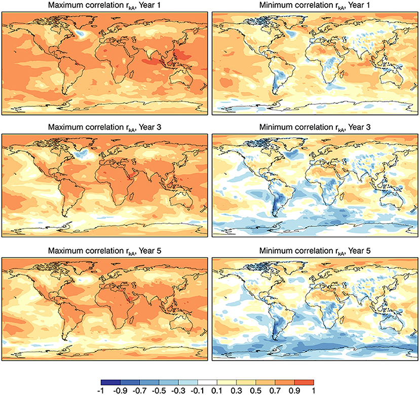
Figure 8. The local maximum and minimum correlation skill r_kA over all reanalysis for Year 1, 3, and 5 ensemble mean forecasts.

The difference between the maximum and minimum correlation skill of the ensemble mean forecast, due to the differences in the data used to verify the forecasts, is quite striking in Figure 8. These upper and lower bounds can arise from different analyses at different points. They represent the best and worst scores available if one were able to choose the corresponding analysis at each point. While this is not directly possible the range of scores illustrates and reiterates that non-trivial differences in apparent skill can arise depending on the verification data set used.

This is illustrated in particular in Figure 9 which plots the correlations r_kA using the HadCRUT5 station-based and the JRA-55 reanalyses as verification data. The skill in both cases declines notably over the oceans although with a more rapid decline in the JRA-55 case for the tropical and northern hemisphere oceans. There is also a difference in the immediate vicinity of Australia where negative skill is seen which extends over part of the land. Differences over land appear at year 1 and evolve subsequently with forecast range although perhaps less so over North America compared to other regions. The overall difference carries over to the global average in Figure 7. It would apparently be beneficial to assess the skill of the current version of the CCCma decadal prediction system using the HadCRUT5 data, at least for annual mean surface air temperature. The verifying observations should of course be the most accurate available and not chosen based on the best agreement with the predictions.

FIGURE 9

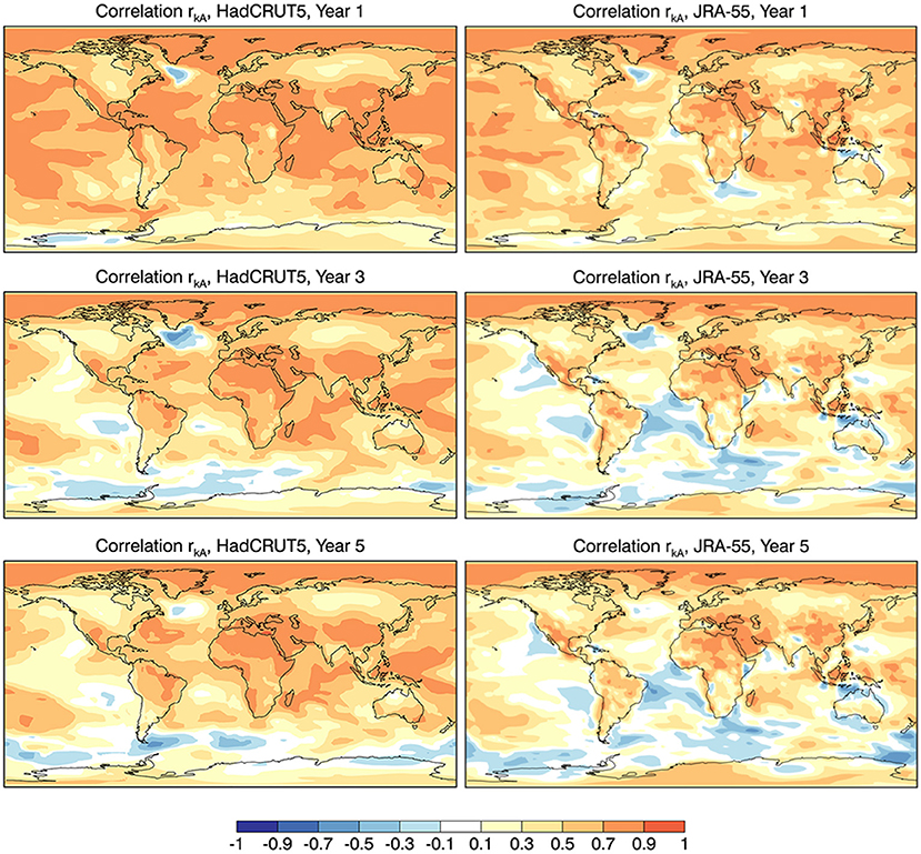
Figure 9. Correlation skill r_kA for the reanalyses with maximum and minimum global averaged correlation skill < r_kA > in Figure 7 for Year 1, 3, and 5 ensemble mean forecasts.

6.3. Skill for Individual Forecasts and Analyses

Although not directly pertinent, it is perhaps of modest interest to consider the upper and lower bounds of the correlations that result when comparing individual ensemble members of the forecast ensemble with individual sources of verifying data, i.e., r_kl in (6). The result is shown in Figure 10. For year 1, even the worst match between forecasts and analyses, the lower bound, has regions of positive skill, although mainly over the oceans, but by year 3 essentially all skill is lost. By contrast, skill for the upper bound is positive virtually everywhere even at year 5. The range of results is impressive which argues for large enough ensembles so as to average out much of the noise in the ensemble mean forecasts and, perhaps, the use of an ensemble average of available verification data so as to average out (some of the) error in the analyses.

FIGURE 10

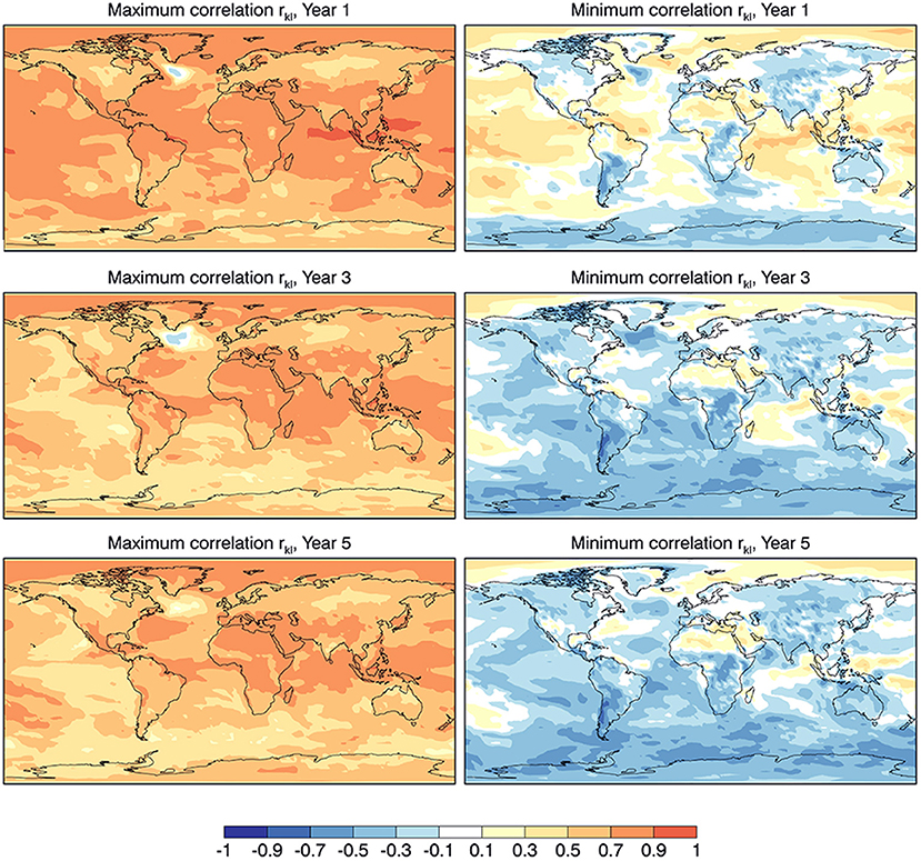
Figure 10. The local maximum and minimum correlation skill r_kl between individual members of the reanalysis X_k and forecast Y_l ensembles for Year 1, 3, and 5.

7. Mean Square Error

The differences in correlation in (6) that depend on the averaging of the forecasts and/or analyses are paralleled by differences in mean square error in (7). Since variances differ among analyses, so too will values of MSE. Figure 11 displays the root mean square error (RMSE) e_AA between the ensemble means of the analyses and forecasts for years 1, 3, and 5. The RMSE increases modestly with forecast range especially at higher latitudes where error is relatively large. The reverse is to some extent the case for regions of the subpolar North Atlantic and Labrador Sea suggesting difficulties in the initialization over these regions (Sospedra-Alfonso and Boer, 2020; Sospedra-Alfonso et al., 2021).

FIGURE 11

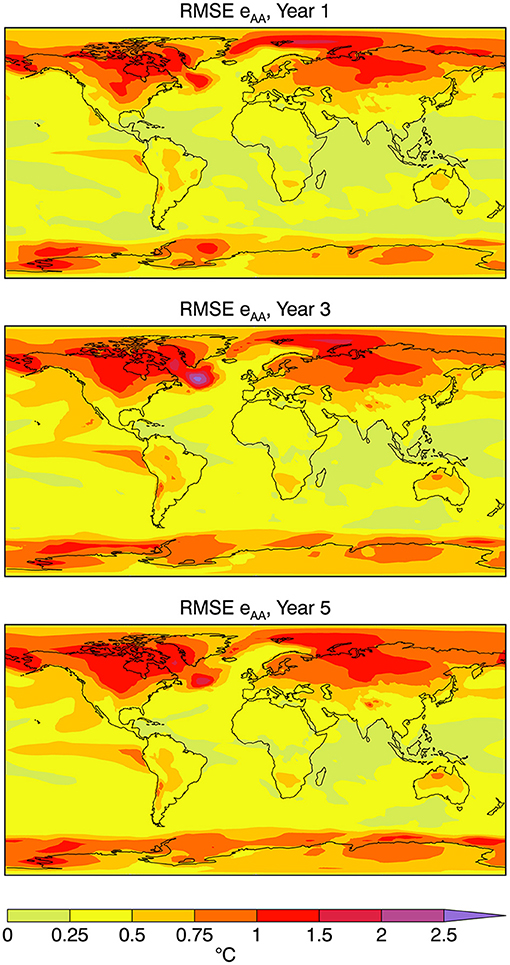
Figure 11. Root mean square error e_AA between the ensemble mean analysis X_A and the ensemble mean forecast Y_A.

Figure 12 displays the upper and lower bounds of the RMSE e_kA between individual analyses and the year 1 ensemble mean forecast. The lower row of Figure 12 plots the RMSE bounds e_kl between individual analyses and year 1 forecasts. The patterns in both Figures 11, 12 resemble that of the standard deviation of the analyses in Figure 3 as would be expected in that larger variations support the possibility of larger errors and differences. The results again illuminate that skill scores can differ depending on the verifying analysis used to calculate them.

FIGURE 12

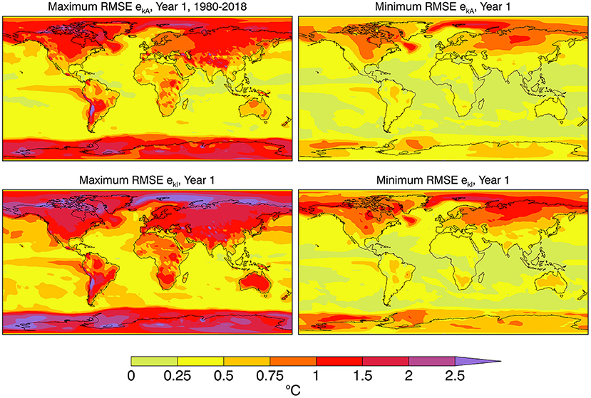
Figure 12. The (left) maximum and (right) minimum root mean square error (top) e_kA of different analyses X_k compared to the ensemble mean forecast Y_A, and (bottom) e_kl of individual analyses X_k and forecast members Y_l for Year 1.

8. Summary

There is increasing interest in climate change and climate prediction on annual to multi-annual timescales based on individual and multi-model approaches. To be of use such forecasts must exhibit skill and this requires verification. Reanalysis and station based sources of gridded climate data are available for verification studies. The current study considers seven reanalyses and four station based analyses of annual mean surface temperature which is a basic decadal prediction variable. The analyses are compared both for the global average and locally. The study additionally investigates the correlation and mean square error scores of decadal forecasts at ranges from 1 to 5 years produced at the Canadian Centre for Climate Modelling and Analysis. The 39 year period 1980–2018 is common to all of the data sets and is used in the analysis.

Globally averaged annual mean temperatures exhibit general warming over the period, roughly characterized by fitting a linear trend to the data, together with variations about the trend. There are visible differences between different analyses which are also seen in their deviations from the ensemble average of the analyses. The magnitudes of the linear trends vary modestly across the analyses with the trends of the station-based analyses somewhat stronger than that of the ensemble mean trend. Half of the trends in the reanalyses are larger and half smaller than the ensemble mean trend. Globally averaged annual mean temperature analyses have about 97% of their variance in common with about 74% of the variance accounted for by the ensemble mean linear trend and 26% by the variation about the trend. The variance of the trends themselves is small at about 1%. Global mean temperature results agree reasonably well among the analyses although the agreement owes much to the trend in temperature associated with global warming.

For geographically distributed annual mean temperatures, anomalies from the long term mean are the variable of interest. The global average of local temporal variability gives a broad measure of overall variability and is seen to differ modestly across analyses. The variances from the reanalyses exceed those from the station-based analyses. Global averages of the local variance components indicate that about 83% of the variance is in common and about 24% is associated with the variance of local trends.

The geographical distribution of the variance exhibits the usual pattern with larger values at higher latitudes and over land. The fraction of the overall variance accounted for by variation about the ensemble mean shows a marked hemispheric difference with larger values in the southern hemisphere and over tropical land, presumably reflecting the asymmetry in the accuracy and availability of the raw data entering the analyses. A pairwise test comparing the variances of the analyses, discounting their common features, indicates that the best agreement is over the extra-tropical oceans and some land areas and the worse agreement is over tropical oceans and at high latitudes (visually associated with ice boundaries).

The differences in correlation and mean square error skill measures for multi-year predictions of annual mean temperature that arise from differences in the verifying data are considered in three ways. The basic measure compares the ensemble average forecast with the ensemble average of the analyses. For correlation this is symbolized as r_AA and the results are reminiscent of those in, e.g., Boer et al. (2013, 2019a), with a general decrease of skill over the first 3–4 years and then a stabilization of the global averaged skill thereafter. This behavior is attributed to the declining skill of the initialized predictable component giving way to the skill of the forced component.

This general behavior applies also to the skill of the ensemble mean forecast as compared to different analyses symbolized as r_kA. For the global means of r_kA the scores using station-based verification data are greater than the global mean of r_AA while the values using reanalyses as verification tend to be lower. The benefit of choosing a “compatible” verification data set is illustrated by contrasting r_kA using the HadCRUT5 analysis as verification compared to using JRA-55 reanalysis as verification. This suggests once again how different sorts of verification data may affect the forecast skill reported by forecasting and modeling centers.

The upper and lower bounds of r_kA are evaluated at each gridpoint. The maximum value of r_kA is greater than that of r_AA while the minimum is lower. The differences between these two values indicate the range of skill values that different verifying analyses can produce locally.

While not particularly pertinent to current decadal prediction systems which forecast ensemble means, the differences are even more notable when plotting the bounds of r_kl, the correlation values comparing single forecasts with single analyses. In this case, the correlation is positive virtually everywhere for the upper bound and negative almost everywhere for the lower bound. These bounds apply locally so are not necessarily associated with an individual analysis, but they nevertheless indicate that a sequence of single forecasts verified with a single verifying data set can “get lucky” or the reverse locally. Similar kinds of results are seen for root mean square error.

An ensemble mean acts to average out unpredictable variance and to improve the skill of a deterministic forecast. However, even for the ensemble mean forecast the calculated skill of the forecast can depend on the analysis used to verify it. This can be problematic when comparing the skill of forecasting systems which are verified with different analyses or even when comparing different versions of the same forecasting system if the verifying analysis does not remain the same. The implication is that some agreed upon verification data set should be used by all modeling centers when verifying decadal forecasting results. The difficulty is in choosing that data set. Of course the “best” data set should be used, if such can be identified and agreed upon. The ensemble mean of available analyses is a straightforward option but the differences between analyses, and the resulting differences in forecast skill, mitigates against this. The ensemble mean of a subset of recent analyses, assumed to be of improved quality, would be another option. Such a standard verification data set could be updated periodically to provide a benchmark against which to verify and intercompare decadal forecasts.

Data Availability Statement

The reanalyses and station-based data used in this study are listed in Table 1 and are publicly available from: ERA-Interim (https://www.ecmwf.int/en/forecasts/datasets/reanalysis-datasets/era-interim, accessed November 28, 2021); ERA5 (https://www.ecmwf.int/en/forecasts/datasets/reanalysis-datasets/era5, accessed October 16, 2021); NCEP-NCAR (https://psl.noaa.gov/data/gridded/data.ncep.reanalysis.html, accessed October 6, 2021); NCEP-DOE (https://psl.noaa.gov/data/gridded/data.ncep.reanalysis2.html, accessed May 25, 2020); CFSR-CFSv2 (https://doi.org/10.5065/D69K487J, accessed March 10, 2020); JRA-55 (https://doi.org/10.5065/D6HH6H41, accessed February 4, 2020); MERRA-2 (https://disc.gsfc.nasa.gov/datasets/M2I1NXASM_5.12.4/summary, accessed March 12, 2020); GISS (https://data.giss.nasa.gov/gistemp/, accessed January 26, 2021); HadCRUT5 (https://www.metoffice.gov.uk/hadobs/hadcrut5/, accessed May 7, 2021); NOAA (10.25921/9qth-2p70, accessed January 26, 2021); Berkeley (http://berkeleyearth.org/data/, accessed January 26, 2021). The data for the CanESM5 decadal experiments (Sospedra-Alfonso et al., 2019) are publicly available from the Earth System Grid Federation (https://esgf-node.llnl.gov/search/cmip6/, accessed October 13, 2021).

Author Contributions

GB initiated the study, preformed a preliminary analysis, and wrote a first draft of the paper. RS-A contributed with the production and assessment of the decadal forecasts used, redid the analysis with an updated set of observation-based products, and produced new versions of the figures. PM and VK contributed with the analysis and the preparation of the reanalyses and station-based data. All authors contributed to the final version of the article.

Funding

PM was supported in part by the Japan Society for the Promotion of Science (JSPS) through Grant-in-Aid for Scientific Research JP19H05702 (on Innovative Areas 6102).

Conflict of Interest

The authors declare that the research was conducted in the absence of any commercial or financial relationships that could be construed as a potential conflict of interest.

Publisher's Note

All claims expressed in this article are solely those of the authors and do not necessarily represent those of their affiliated organizations, or those of the publisher, the editors and the reviewers. Any product that may be evaluated in this article, or claim that may be made by its manufacturer, is not guaranteed or endorsed by the publisher.

Acknowledgments

We are thankful to James Anstey for helpful comments on an earlier version of this paper. We acknowledge the various organizations listed in Table 1 for making their data freely available.

References

Boer, G. J., Kharin, V. V., and Merryfield, W. J. (2013). Decadal predictability and forecast skill. Clim. Dyn. 41, 1817–1833. doi: 10.1007/s00382-013-1705-0

CrossRef Full Text | Google Scholar

Boer, G. J., Kharin, V. V., and Merryfield, W. J. (2019a). Differences in potential and actual skill in a decadal prediction experiment. Clim. Dyn. 52, 6619–6631. doi: 10.1007/s00382-018-4533-4

CrossRef Full Text | Google Scholar

Boer, G. J., Merryfield, W. J., and Kharin, V. V. (2019b). Relationships between potential, attainable, and actual skill in a decadal prediction experiment. Clim. Dyn. 52, 4813–4831. doi: 10.1007/s00382-018-4417-7

CrossRef Full Text | Google Scholar

Boer, G. J., Smith, D. M., Cassou, C., Doblas-Reyes, F., Danabasoglu, G., Kirtman, B., et al. (2016). The Decadal Climate Prediction Project (DCPP) contribution to CMIP6. Geosci. Mod. Dev. 9, 3751–3777. doi: 10.5194/gmd-9-3751-2016

CrossRef Full Text | Google Scholar

Dee, P., Uppala, S. M., Simmons, A. J., Berrisford, P., Poli, P., Kobayashi, S., et al. (2011). The ERA-Interim reanalysis: configuration and performance of the data assimilation system. Q. J. R. Meteorol. Soc. 137, 553–597.

Google Scholar

Eyring, V., Bony, S., Meehl, G. A., Senior, C. A., Stevens, B., Stouffer, R. J., et al. (2016). Overview of the coupled model intercomparison project phase 6 (CMIP6) experimental design and organization. Geosci. Model Dev. 9, 1937–1958. doi: 10.5194/gmd-9-1937-2016

CrossRef Full Text | Google Scholar

Fujiwara, M., Wright, J. S., Manney, G. L., Gray, L. J., Anstey, J., Birner, T., et al. (2017). Introduction to the SPARC Reanalysis Intercomparison Project (S-RIP) and overview of the reanalysis systems. Atmos. Chem. Phys. 17, 1417–1452. doi: 10.5194/acp-17-1417-2017

CrossRef Full Text | Google Scholar

Gelaro, R., McCarty, W., Suarez, M. J., Todling, R., Molod, A., Takacs, L., et al. (2017). The 20 Modern-Era Retrospective Analysis for Research and Applications, version 2 (MERRA-2). J. Clim. 30, 5419–5454. doi: 10.1175/JCLI-D-16-0758.1

PubMed Abstract | CrossRef Full Text | Google Scholar

Goddard, G. J., Kumar, A., Solomon, A., Smith, D., Boer, G., González, P., et al. (2013). A verification framework for interannual-to-decadal predictions experiments. Clim. Dyn. 40, 245–272. doi: 10.1007/s00382-012-1481-2

CrossRef Full Text | Google Scholar

Hartmann, D., Tank, A. K., Rusticucci, M., Alexander, L., Bronnimann, S., Charabi, Y., et al. (2013). “Observations: atmosphere and surface,” in Climate Change 2013: The Physical Science Basis. Contribution of Working Group I to the Fifth Assessment Report of the Intergovernmental Panel on Climate Change (Cambridge University Press).

Google Scholar

Hermanson, L., Smith, D., Seabrook, M., Bilbao, R., Doblas-Reyes, F., Tourigny, E., et al. (2022). WMO global annual to decadal climate update: a prediction for 2021-2025. Bull. Am. Meteorol. Soc.

Hersbach, H., Bell, B., Berrisford, P., Hirahara, S., Horanyi, A., Munoz-Sabater, J., et al. (2020). The ERA5 global reanalysis. Q. J. R. Meteorol. Soc. 146, 1999–2049. doi: 10.1002/qj.3803

CrossRef Full Text | Google Scholar

Huang, B., Menne, M. J., Boyer, T., Freeman, E., Gleason, B. E., Lawrimore, J. H., et al. (2020). Uncertainty estimates for sea surface temperature and land surface air temperature in NOAAGlobalTemp version 5. J. Clim. 33, 1351–1379. doi: 10.1175/JCLI-D-19-0395.1

PubMed Abstract | CrossRef Full Text | Google Scholar

Jolliffe, I. T., and Stephenson, D. B. (2012). Forecast Verification:A Practitioner's Guide in Atmospheric Science. Chichester: Wiley and Sons Ltd. doi: 10.1002/9781119960003

CrossRef Full Text | Google Scholar

Kalnay, E., Kanamitsu, M., Kistler, R., Collins, W., Deaven, D., Gandin, L., et al. (1996). The NCEP/NCAR 40-year reanalysis project. Bull. Am. Meteorol. Soc. 77, 437–471. doi: 10.1175/1520-0477(1996)077<0437:TNYRP>2.0.CO;2

CrossRef Full Text | Google Scholar

Kanamitsu, M., Ebisuzaki, W., Woollen, J., Yang, S.-K., Hnilo, J. J., Fiorino, M., et al. (2002). NCEP-DOE AMIP- II reanalysis (R-2). Bull. Am. Meteorol. Soc. 83, 1631–1644. doi: 10.1175/BAMS-83-11-1631

CrossRef Full Text | Google Scholar

Kirtman, B., Power, S., Adedoyin, J., Boer, G., R. Bojariu, I. C., Doblas-Reyes, F., et al. (2013). “Near-term climate change: projections and predictability,” in Climate Change 2013: The Physical Science Basis. Contribution of Working Group I to the Fifth Assessment Report of the Intergovernmental Panel on Climate Change (Cambridge University Press).

Google Scholar

Kobayashi, S., Ota, Y., Harada, Y., Ebita, A., Moriya, M., Onoda, H., et al. (2015). The JRA-55 reanalysis: general specifications and basic characteristics. J. Meteorol. Soc. Japan II 93, 5–48. doi: 10.2151/jmsj.2015-001

CrossRef Full Text | Google Scholar

Kushnir, Y., Scaife, A. A., Arritt, R., Balsamo, G., Boer, G., Doblas-Reyes, F., et al. (2019). Towards operational predictions of the Near-Term Climate. Nat. Clim. Change 9, 94–101. doi: 10.1038/s41558-018-0359-7

CrossRef Full Text | Google Scholar

Lenssen, N., Schmidt, G., Hansen, J., Menne, M., Persin, A., Ruedy, R., et al. (2019). Improvements in the GISTEMP uncertainty model. J. Geophys. Res. 12, 6307–6326. doi: 10.1029/2018JD029522

CrossRef Full Text | Google Scholar

Martineau, P., Wright, J. S., Zhu, N., and Fujiwara, M. (2018). Zonal-mean data set of global atmospheric reanalyses on pressure levels. Earth Syst. Sci. Data 10, 1925–1941. doi: 10.5194/essd-10-1925-2018

CrossRef Full Text | Google Scholar

Morice, C. P., Kennedy, J. J., Rayner, N. A., Winn, J. P., Hogan, E., Killick, R. E., et al. (2021). An updated assessment of near-surface temperature change from 1850: the HadCRUT5 data set. J. Geophys. Res. Atmos. 126, e2019JD032361. doi: 10.1029/2019JD032361

CrossRef Full Text | Google Scholar

Pitman, J. G.. (1939). A note on normal correlation. Biometrika 31, 9–12. doi: 10.1093/biomet/31.1-2.9

CrossRef Full Text | Google Scholar

Rohde, R. A., and Hausfather, Z. (2020). The Berkeley earth land/ocean temperature record. Earth Syst. Sci. Data 12, 3469–3479. doi: 10.5194/essd-12-3469-2020

CrossRef Full Text | Google Scholar

Saha, S., Moorthi, S., Pan, H.-L., Wu, X., Wang, J., Nadiga, S., et al. (2010). The NCEP climate forecast system reanalysis. Bull. Am. Meteorol. Soc. 91, 1015–1057. doi: 10.1175/2010BAMS3001.1

CrossRef Full Text | Google Scholar

Smith, D. M., Scaife, A. A., Boer, G. J., Caian, M., Doblas-Reyes, F. J., Guemas, V., et al. (2013). Real-time multi-model decadal climate predictions. Clim. Dyn. 41, 2875–2888. doi: 10.1007/s00382-012-1600-0

CrossRef Full Text | Google Scholar

Sospedra-Alfonso, R., and Boer, G. J. (2020). Assessing the impact of initialization on decadal prediction skill. Geophs. Res. Lett. 47, e2019GL086361. doi: 10.1029/2019GL086361

CrossRef Full Text | Google Scholar

Sospedra-Alfonso, R., Lee, W., Merryfield, W. J., Swart, N. C., Cole, J. N. S., Kharin, V. V., et al. (2019). CCCma CanESM5 Model Output Prepared for CMIP6 DCPP DCPPA-Hindcast. Earth System Grid Federation.

Sospedra-Alfonso, R., Merryfield, W. J., Boer, G. J., Kharin, V. V., Lee, W.-S., Seiler, C., et al. (2021). Decadal climate predictions with the Canadian Earth System Model version 5 (CanESM5). Geosci. Model Dev. 14, 6863–6891. doi: 10.5194/gmd-14-6863-2021

CrossRef Full Text | Google Scholar

Taylor, K. E., Stouffer, R. J., and Meehl, G. A. (2012). An overview of CMIP5 and the experiment design. Bull. Am. Meteorol. Soc. 93, 485–498. doi: 10.1175/BAMS-D-11-00094.1

CrossRef Full Text | Google Scholar

WMO (2016). Use of Climate Predictions to Manage Risks. Technical Report 1174, World Metheorological Organization.

Zhang, H.-M., Lawrimore, J. H., Huang, B., Menne, M. J., Yin, X., Sánchez-Lugo, A., et al. (2019). Updated temperature data give a sharper view of climate trends. Eos 100. doi: 10.1029/2019EO128229

CrossRef Full Text | Google Scholar