Parameter Estimation Using Adaptive Observations Toward Maximum Total Variance Reduction With Ensemble Adjustment Kalman Filter

In real applications, one common issue of parameter estimation using ensemble-based data assimilation methods is the accumulation of sampling errors when a large number of observations are used to update single-value parameters. In this article, a new parameter estimation method which assimilates a large number of observations to estimate the states while assimilates adaptive observations to update the parameters is introduced. The observations resulting in maximum total variance reduction to the parameter ensembles are identified to perform parameter estimation. To validate this new method, the two-scale Lorenz-96 model is used to generate true states, while a parameterized one-scale Lorenz-96 model is used to perform state and parameter estimation experiments. The comparison between state estimation and parameter estimation with fixed or adaptive observations shows the new method can be more effective in estimating the model parameters and providing more accurate analyses. This method also shows its potential to be used in the data assimilation with large general circulation models to better produce reanalyzes.

1. Introduction

In numerical weather prediction and ocean circulation simulations, parametrizations are used to simulate missing physics due to a lack of scientific understanding or a lack of computational powers. It is well acknowledged that many parameters used in the parameterization are derived from the empirical relations, which are intrinsically uncertain. The uncertainty in some parameters contributes to model errors, that may have great impacts on the model performance (Tong and Xue, 2008; Furue et al., 2015).

Parameter estimation (PE) is defined as the process of adjusting and optimizing uncertain model parameters using observations. Similar to state estimation (SE) which corrects the model states by observations, PE can be done with data assimilation (DA) methods. In ensemble-based data assimilation methods for PE, such as the ensemble Kalman filter (EnKF) and local ensemble transform Kalman filter (LETKF), the uncertain parameters are regarded as special state variables and augmented to the ensemble of background states. To update the augmented ensemble, DA schemes are employed either simultaneously or separately. Simultaneous PE techniques update the model states and parameters concurrently by some DA method, while separate PE techniques update the ensembles of states and parameters independently in different stages (e.g., Koyama and Watanabe, 2010).

Since most parameters are connected to the observed model states indirectly, the PE problems are always nonlinear and thus very difficult in practical. Zhang et al. (2020) reviewed the recent progress and challenges of PE, particularly with complicated coupled general circulation models. One major challenge of PE is that some parameters take globally uniform values and thus assimilating numerous data to estimate those scalar parameters would over-adjust their values and bring unexpected errors. To deal with this issue, Wu et al. (2013) developed the geographic-dependent parameter optimization (GPO) which allows model parameters to vary geographically in particular models. For more general scenarios, Aksoy et al. (2006) proposed a method that first transforms the single-value parameter into a two-dimensional field and then updates the field spatially in the analysis step. After the PE step, a spatial average (SA) of the entire spatially varying parameter field is used to recover the globally uniform parameter value for model integration. To speed up the converge of the parameter ensemble, Liu et al. (2014a) proposed an adaptive spatial average (ASA) method which computes the average parameter in areas with the most significant observation impacts.

It is obvious that the most prominent contradiction in PE with a high-dimensional model is that the large dimension of state space requires a large number of observation data and that the massive quantities of observational data lead to excessive parameter corrections. The mentioned methods attempt to extend the dimension of the parameter space, then use posterior values of the parameters in the extended form (GPO) or the averaged value over a specific region (ASA). Both methods are widely used in applications of PE with coupled general circulation models, e.g., Liu et al. (2014b); Li et al. (2018); Shen and Tang (2022). However, it is still a waste of computing resources by extending the parameter space during the analysis step if it is possible to reduce the number of observations for the estimation of parameters.

This work aims to introduce a new PE method which can assimilate adaptive observations to estimate the uncertain parameters. The adaptive observations, also known as targeted observations, result from the target observation methods, which locate observations to optimally improve the state estimation and forecast accuracy (Emanuel et al., 1995; Bergot, 2010; Pu and Kalnay, 2010).

Many target observation approaches exist for adaptive observing purposes and can generally be divided into two categories (Wu et al., 2020). The first kind of approach aims to locate observations where the solutions of a dynamical system exhibit instability. The most common techniques in this category include the singular vector (SV) (Palmer et al., 1998), breeding vector (BV) (Toth and Kalnay, 1997), conditional nonlinear optimal perturbation (CNOP) (Mu et al., 2003), and nonlinear forcing singular vector (NFSV) (Duan and Zhou, 2013) methods.

The second kind of approach incorporates data assimilation (DA) methods (such as ensemble transform techniques) (Bishop and Toth, 1998) to determine where to target an additional observation (Torn and Hakim, 2008). These methods independently simulate an observation at each possible observational location and perform a DA analysis for each observation. Each independent DA analysis has a corresponding state error covariance, and the particular observation resulting in the smallest state error covariance is chosen as the location of the targeted observation. These methods are frequently used in real applications because they do not need a complicated adjoint model and are easy to implement (Whitaker et al., 2008).

Although target observation methods were originally designed for SE, they have recently been applied for PE. For example, Bellsky et al. (2014) performed target observation methods for PE using a separate scheme, in which LETKF is used for state variables and EnKF is used for parameters. They indicate that using the LETKF and EnKF with observations targeted at the locations of greatest ensemble variance is skillful at reducing analysis error for the Lorenz-96 model. However, they assimilate the same observations with different schemes for state and parameter ensembles, which is not helpful to cope with the problem of excessive parameter corrections.

In this work, a new PE method which assimilates the full set of observations for state variables and assimilates targeted observations for parameters is introduced. The target observation method is developed with the ensemble adjustment Kalman filter (EAKF) to identify the locations of the adaptive observations. The total variance reduction (TVR) is defined to measure the influence of each observation to the parameters, which is chosen to update the model parameters. The derived formulas have very strong connection with the criterion for selecting good values in the widely-used ASA method. The twin experiments using a two-scale Lorenz-96 model and a parameterized Lorenz-96 model are conducted to validate the new PE method.

The remainder of this article is organized as follows. The PE method combined with targeted observation is described in Section 2. The models and experimental designs are introduced in the first part of Section 3, and Sections 3.2 show the results with some discussion. In Section 4, our conclusions are finally drawn.

2. Methods

In this work, the serial version of EAKF is used to perform joint state and parameter estimation. The EAKF is first introduced by Anderson (2001) as a deterministic ensemble filtering method. Later, a local least squares framework has been derived leading to a two-step ensemble filtering update procedure that can assimilate the observations sequentially (Anderson, 2003). EAKF has been successfully implemented in many large geophysical application, since it greatly reduces computational requirements, and lead to good assimilations with a relatively small ensemble (Anderson, 2009a). The serial EAKF uses each observation to update the state variable entries and parameters one after another, such that the estimation of state variables and parameters can be separated.

In the following, x denotes the state vector, θ denotes the uncertain parameters as a vector, y^o denotes a single scalar observation with variance R, and h is denotes the measurement operator. The ensembles of x and θ are updated with a two-step procedure, which first computes the observational increments according to the disparities of model projection and observation, then regression the observational increments to the state/parameter space. The augmented method for PE implies that the measurement operator h project both x and θ to the observational space, i.e.,

$\begin{array}{ll}{y}_n^p=h(x_n^p;{\theta }_n^p),n=1,...,N,& (1)\end{array}$

where the superscript p indicates the prior value, n is the index of the ensemble member, and N is the ensemble size.

The scheme for updating the state vector x refers to Anderson (2003), and the corresponding adaptive inflation method refers to Anderson (2009b). This work focus on the update of the parameter ensemble {θ_n, n = 1, 2, …, N}.

As the same as state estimation, the observational increment can be computed as

$\begin{array}{ll}{y}_n^u-\overline{y^u}=(\frac{{\sigma }_y^u}{{\sigma }_y^p})(y_n^p-\overline{y^p}),n=1,...,N,& (2)\end{array}$

where the posterior ensemble mean

$\begin{array}{ll}\overline{y^u}={({\sigma }_y^u)}^2\left[\frac{\overline{y^p}}{{({\sigma }_y^p)}^2}+\frac{y^o}{R}\right].& (3)\end{array}$

and posterior ensemble variance

$\begin{array}{ll}{({\sigma }_y^u)}^2=\frac{{({\sigma }_y^p)}^{2}R}{{({\sigma }_y^p)}^2+R}& (4)\end{array}$

are explicitly derived from the prior.

The EAKF linearly regresses the prior ensemble sample of each parameter on the observation variable to compute the update increments for each parameter ensemble member from the corresponding observational variable increments. The nth posterior parameter ensemble member for the parameter indexed by m, denoted ${\theta }_{m,n}^u$, can be updated by

$\begin{array}{ll}{\theta }_{m,n}^u={\theta }_{m,n}^p+\frac{{\Sigma }_{{\theta }_m,y}}{{({\sigma }_y^p)}^2}(y_n^u-y_n^p).& (5)\end{array}$

where Σ_{θm, y} is the covariance between ${\theta }_m^p$ and y^p. It is noteworthy that a localization factor ρ is always multiplied to the second term on the right-hand-side for state estimation to apply covariance localization. However, since we assume that the parameters are globally uniform, localization is not necessary for each θ. If we substitute the relation ${\Sigma }_{{\theta }_m,y}=r_{{\theta }_m,y}{\sigma }_{{\theta }_m}^p*{\sigma }_y^p$ into Equation (5), where r_{θm, y} is the correlation coefficient between θ_m and the prior projection y^p, the equation can be simplified to

$\begin{array}{ll}{\theta }_{m,n}^u={\theta }_{m,n}^p+\rho *r_{\theta ,y}\frac{{\sigma }_{\theta }^p}{{\sigma }_y^p}(y_n^u-y_n^p),& (6)\end{array}$

Using Equation (6), it is easy to calculate the posterior error variance of each parameter. We first compute the mean value of ${\theta }_{m,n}^u$ for n = 1, 2, …, N and then subtract it from Equation (6):

$\begin{array}{ll}({\theta }_{m,n}^u-\overline{{\theta }_m^u})==({\theta }_{m,n}^p-\overline{{\theta }_m^p})+r_{{\theta }_m,y}\frac{{\sigma }_{{\theta }_m}^p}{{\sigma }_y^p}(\frac{{\sigma }_y^u}{{\sigma }_y^p}-1)(y_n^p-\overline{y^p}),& (7)\end{array}$

in which Equation (2) is substituted.

Squaring both sides of Equation (7) and averaging them, it can be derived that

$\begin{array}{ll}{({\sigma }_{{\theta }_m}^u)}^2={({\sigma }_{{\theta }_m}^p)}^2\left\{1+r_{{\theta }_m,y}^2\left[{(\frac{{\sigma }_y^u}{{\sigma }_y^p})}^2-1\right]\right\}.& (8)\end{array}$

Upon substituting Equation (4), Equation (8) can be rewritten as

$\begin{array}{ll}{({\sigma }_{{\theta }_m}^p)}^2-{({\sigma }_{{\theta }_m}^u)}^2={({\sigma }_{{\theta }_m}^p)}^2{r}_{{\theta }_m,y}^2\left[1-{(\frac{{\sigma }_y^u}{{\sigma }_y^p})}^2\right]={({\sigma }_{{\theta }_m}^p)}^2{r}_{{\theta }_m,y}^2\frac{{({\sigma }_y^p)}^2}{{({\sigma }_y^p)}^2+R}.& (9)\end{array}$

Equation (9) evaluates the reduction in the variance of the parameter θ_m when an observation with variance R is assimilated. This implies that the variance reduction (VR) of the variable parameter is proportional to its prior variance, the square of its correlation coefficient with the observed variable, and the regression coefficient of the posterior variance in the observational space. Liu et al. (2014a) indicates that the value of $\Omega =r_{{\theta }_m,y}^2\frac{{({\sigma }_y^p)}^2}{{({\sigma }_y^p)}^2+R}$ can be a criterion for selecting good values from the posterior of the extended parameter ensemble, since Equation (9) can be written as ${({\sigma }_{{\theta }_m}^u)}^2={({\sigma }_{{\theta }_m}^p)}^2(1-\Omega )$. In their PE method, the parameter θ_m is firstly extended to a vector with spatial dependence, then updated locally using all observations (with covariance localization), and finally averaged over areas in which Ω is larger than a prescribe threshold.

The current method first assimilates the entire observation dataset to update the model state, then assimilate adaptive observation to update the parameters. For this purpose, the total variance reduction (TVR) from one observation to all the undetermined parameters is defined as

$\begin{array}{ll}\text{TVR}(y^o)=\underset{m=1}{\overset{M}{{{\displaystyle \sum }}^{\text{}}}}[{({\sigma }_{{\theta }_m}^p)}^2-{({\sigma }_{{\theta }_m}^u)}^2]=\frac{{({\sigma }_y^p)}^2}{{({\sigma }_y^p)}^2+R}\underset{m=1}{\overset{M}{{{\displaystyle \sum }}^{\text{}}}}{({\sigma }_{{\theta }_m}^p)}^2{r}_{{\theta }_m,y}^2,& (10)\end{array}$

that can be used to measure the impact of one observation to all those parameters. The observational site with the largest TVR is expected to maximally reduce the uncertainties in parameters such that this site can be identified as the location of an adaptive observation (Huan and Marzouk, 2013; Gharamti et al., 2015). This procedure, which is very effective in practice, can be applied repeatedly to find more other observational sites once the identified adaptive observation is assimilated (Sakov and Oke, 2008). Assimilating a sufficient number of observations could be most effective to update the parameters while not introduce the problem of excessive corrections.

In the following section, this newly developed PE method is validated with a parameterized Lorenz-96 model.

3. Numerical Experiments

3.1. Twin Experiment Settings

In the DA community, the Lorenz-96 model is a simple model that is frequently used as a testbed for DA methods. The two-scale Lorenz-96 model is an extension of the original Lorenz-96 model that was originally introduced to simulate mid-latitude weather phenomena and to study the influences of multiple spatiotemporal scales on the predictability of atmospheric flows. The two-scale Lorenz-96 model consists of large-scale variables ${\left\{X_k\right\}}_{k=1}^K$ coupled to J*K small-scale variables ${\left\{Z_{j,k}\right\}}_{(j,k)=(1,1)}^{(J,K)}$, whose evolution is governed by

$\begin{array}{ll}\frac{d{X}_k}{dt}=-X_{k-1}(X_{k-2}-X_{k+1})-X_k+F-\frac{hc}{b}{\displaystyle \sum _{j=1}^J}{Z}_{j,k},& (11)\end{array}$

$\begin{array}{ll}\frac{d{Z}_{j,k}}{dt}=cb{Z}_{j+1,k}(Z_{j-1,k}-Z_{j+2,k})-c{Z}_{j,k}+\frac{hc}{b}{X}_k,& (12)\end{array}$

where both X_k and Z_{j, k} are assumed to be periodic, that is, X_k+K = X_k and Z_{j, k+K} = Z_{j, k}, Z_{j+J, k} = Z_{j, k+1}.

Similar to Wilks (2005), the coupled model is used to define the “truth,” i.e., the quantities to be predicted. Here, K = 8 and J = 16, so there are JK = 128 Z variables in total for the truth run. The scaling constants h, c, and b are taken to be 1, 10, and 10, respectively, and F is a forcing term taken to be 8 in the following. The coupled model is integrated with a step size of δt = 0.005 model time units (TUs), which is equal to 36 min in reality. The integration starts from random initial values and runs for 144,000 steps (≈10 years) to allow fluctuations in the system to develop sufficiently. Likewise, the duration of the truth run is 100 TUs (or 20,000 model steps).

In the experiments, the X variables in Equation (11) are regarded as “resolved,” whereas the Z variables governed by Equation (12) are regarded as “unresolved.” Hence, a parameterization scheme is required to mimic the effect of the last coupling term in Equation (11). The parameterized Lorenz-96 model can be written as

$\begin{array}{ll}\frac{\text{d}{X}_k^{*}}{\text{d}t}=-X_{k-1}^{*}(X_{k-2}^{*}-X_{k+1}^{*})-X_k^{*}+F-g_U(X_k^{*})& (13)\end{array}$

for each k, and g_U is the parameterization function. For simplicity, we assume that g_U is a quadratic polynomial with three uncertain coefficients, i.e.,

$\begin{array}{ll}{g}_U(X_k^{*})=b_0+b_1{X}_k^{*}+b_2{(X_k^{*})}^2.& (14)\end{array}$

These coefficients could be regarded as the parameters of the parameterization function whose uncertainties result in model errors. According to Wilks (2005), the reference values of these parameters can be estimated with polynomial fitting. As shown in Figure 1A, the polynomial function with reference coefficients B = [b₀, b₁, b₂] can be calculated by polynomial fitting using the true X and Z values. Therefore, the reference parameters are 0.1232, 1.0401, and -0.0879. However, these true values cannot be obtained without true Z data, so we adopt the initial estimates of these parameters for the experiments, namely, B₀ = [0.1, 1, −0.1], which are slightly different from the reference values.

FIGURE 1

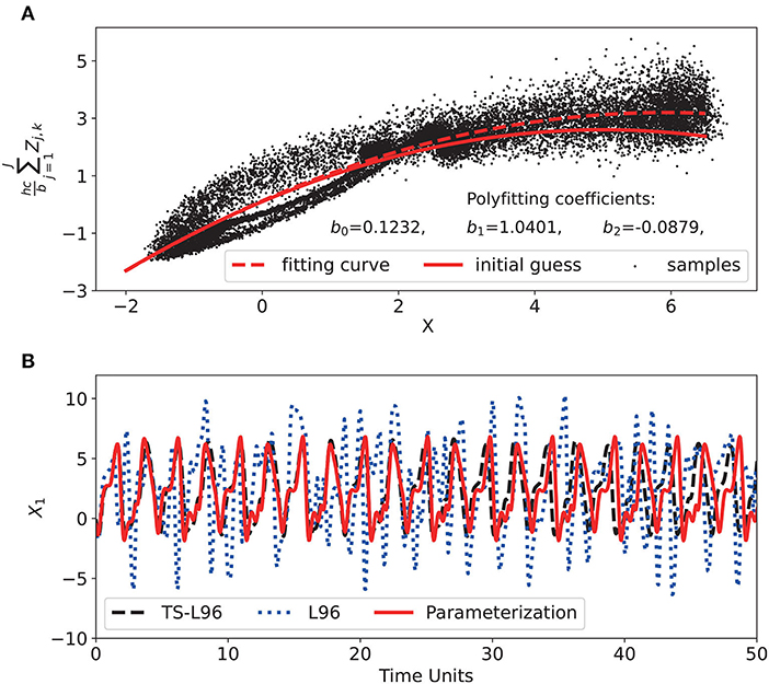
Figure 1. (A) Scatter plot of the effect of unresolved Z variables as a function of the resolved X variables, together with the regression functions constituting the parameterization. (B) Control run of the parameterized Lorenz-96 model (red solid line) and the truncated Lorenz-96 model (blue dotted line) for variable x₁.

In addition, the model step size for the parameterized Lorenz-96 model is Δt = 0.05 TUs (or 6 h), which means that the temporal resolution of the control run is also lower than that of the truth run. As demonstrated in Figure 1B, compared to the truncated Lorenz-96 model, which uses no parameterization, the B₀-parameterized Lorenz-96 model can effectively simulate the X variables of the two-scale model, especially for the first 20 TUs. As a result, B₀ is used during the SE experiment, and it is also used to generate the parameter ensemble in PE.

The observation for each variable is generated every 4 model steps with random observational errors drawn from the Gaussian distribution N(0;0.5) such that R = 0.25 for each observation, and the duration of the DA experiment is 100 TUs (or 2,000 parameterized model steps). To better simulate the situation in practical ensemble data assimilation, a 30-member ensemble generated by the normal distribution $N(x_0^{*},\sqrt{2})$ is used to perform both SE and PE, where $x_0^{*}$ represents the perturbed initial condition or the first observation. The parameterized Lorenz-96 model contains only 8 model variables, we assume that all 8-variables are observed to estimate the states, but only 2 observations are used to estimate the parameters.

3.2. Results

We first perform state estimation only (SEO) experiment, in which the fixed parameters B₀ = [0.1, 1, −0.1] are used in the integration of each ensemble member. The EAKF with adaptive inflation scheme (Anderson, 2009b) is employed to perform SE. Localization is a frequently-used approach in ensemble-based data assimilation methods, since it can suppress long-distance correlations due to insufficient ensemble members (Hunt et al., 2007). In this experiment, the covariance localization method using the Gaspri-Cohn function (Gaspari and Cohn, 1999) is applied with different cut-off parameters. Table 1 compares the root-mean-squared-errors (RMSE) and root-mean-squared-spreads (RMSS) over the state variables of the SE experiments using the same initial ensemble against different cut-off parameters. The mean RMSE and RMSS over the last 75 TUs (1,500 model steps) are computed to measure the performance of each experiment.

TABLE 1

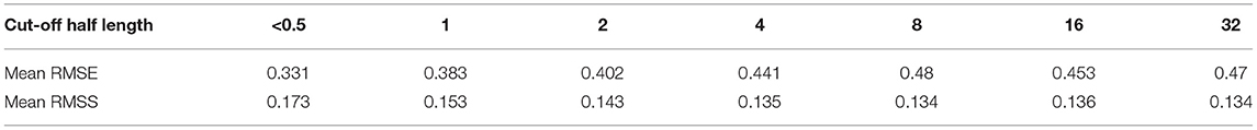
Table 1. The mean RMSE and RMSS against the localization cut-off parameter.

With the cut-off half length c smaller than 0.5, the observation of each variable can only affect itself for this model. However, since it produces the most accurate state estimation, we use this strategy (c = 0.5 ) in the SEO experiment and the state estimation stages of the PE experiment.

Two PE experiments are conducted. In each PE experiment, the initial parameter vector B₀ = [0.1, 1, −0.1] is perturbed with random Gaussian errors with standard deviation [0.2,0.4,0.2] to generate a parameter ensemble with 30 members. Each parameter ensemble member is accompanied with a state ensemble member in the model integration. Zhang et al. (2012) emphasizes that a pure SE procedure is crucially important before PE can be activated to effectively update the parameters. In the PE experiments, we first perform pure SE for 25 TUs, then apply PE with 2 observations after each SE step. For Exp-PEf, the observations of x₂ and x₆ are used to update the parameter ensemble. By contrast, Exp- PEa uses the adaptive observations with maximal TVR to the parameters. As mentioned, no localization strategy is applied to parameters, because they are assumed to be global. And inflation with constant factor 1.02 is used to the parameter ensemble to prevent the degeneracy of the parameter ensemble (Shen and Tang, 2022).

The details of the three experiments are listed in Table 2. Figure 2 shows the errors of the ensemble mean of the data assimilation results against the true values, as the function of model variables and model steps. In Figures 2B,C, the PE procedure starts after 25 TUs. Since the parameter ensemble with initially large variance is used in those PE experiments, the errors and spreads of the state ensembles in Figures 2B,C are much larger than Figure 2A for the first 25 TUs. The RMSE and RMSS are computed and their mean values over the period (0 < t < 25TUs) are also displayed in Figure 2 to quantify this conclusion. The spatially and temporally varying adaptive covariance inflation method (Anderson, 2009b) is adopted in all experiments, such that the inflation factors vary with time and spatial locations. Figure 3 shows the corresponding inflation factors for each experiment. It can be seen from Figures 3B,C that the inflation factors are very small for the PE experiments in the initial SE stage, since the state ensemble spread grows rapidly due to the variety of parameters.

TABLE 2

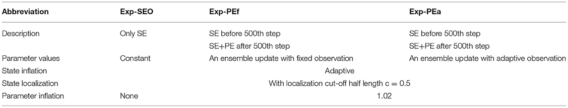
Table 2. Settings of three experiments.

FIGURE 2

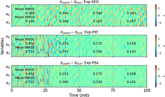
Figure 2. The errors of the assimilated ensemble mean against the true values for Exp-SEO (A), Exp-PEf (B), and Exp-PEa (C).

FIGURE 3

Figure 3. The inflation factors derived from a spatially and temporally varying adaptive inflation method for experiments Exp-SEO (A), Exp-PEf (B), and Exp-PEa (C).

When t>25TUs, the errors and spreads decrease gradually in PE experiments. This is because of the effect of PE, which reduces the uncertainty in the parameter ensembles. The parameters are adjusted according to two observations, thus the model errors during integration can be much smaller than the SEO experiment. The errors of the two PE experiments are much smaller than that of the SEO experiment, as Figure 2 shown. It is even more significant when t>50TUs, a stage that parameter estimation reaches a “steady state”. In addition, since the model errors due to uncertain parameters are greatly reduced, the adaptive inflation factors can also be very small in Figures 3B,C.

In Figures 2B,C, the difference between Exp-PEf and Exp-PEa can be seen in the interval between 25TUs and 50TUs. Using the adaptive observation, the uncertainty of the parameter decreases more rapidly, such that PE reaches the “steady state” earlier than the case using fixed observations. However, although PEf is less effective than PEa, they eventually estimate the parameters to the same level, thus the accuracies of state variables are very similar.

We further investigate the specific locations of the adaptive observations in Figure 4. In the proposed method, when the state estimation is finished with full observations, the TVR defined by Equation (10) is computed for each observational site. Then the one with the largest TVR is chosen as the location of the first adaptive observation. The adaptive observation is immediately assimilated to update the parameters θ_m, and the corresponding standard deviations σ_θm are also update. The procedure is then repeated to identify and assimilate the second adaptive observation. The observational sites from 25TUs are plotted for 125 DA cycles (or 25 TUs). Figure 4 also shows the true values of the X and Z variables, and it is very clear that most adaptive observations are in areas with relatively large X variables. According to the model equations, the Z variable tends to propagate in the direction opposite to the direction that the X variable propagates. Because of the coupling in Equation (12), the Z variables are restricted in areas with large X values and rapidly disappear as they leave these areas (Lorenz, 1996). This implies that the Z variables are most active in areas containing large X variables. The uncertainty of the parameterization is apparently greatest in these areas, such that the observed variables therein could reduce most of the parameter uncertainties. These experiments clearly demonstrate that the new target observation method can effectively identify these observational sites.

FIGURE 4

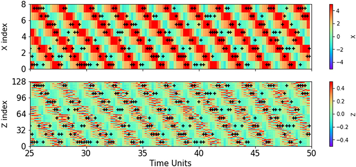
Figure 4. Locations of the adaptive observations for PE with the true states of the resolved X variables (A) and unresolved Z variables (B).

Figure 5 shows the ensemble spread of each parameter during the PE experiments. For both PEf and PEa, the spreads maintain constant until the parameter estimation is activated in 25TUs. The comparison between PEf and PEa indicates that adaptive observation can more effectively reduce the parameter ensemble spread, such that the uncertainty of each parameter with PEa is much smaller than that with PEf. That partly explains why the errors and spreads are smaller for the period 25TUs<t < 50TUs in Figure 2C than that in Figure 2B.

FIGURE 5

Figure 5. The parameter ensemble spreads for parameters b0 (A), b1 (B), b2 (C) with fixed or adaptive observations for PE.

Similar to Figures 1B, 6A shows the effects of unresolved variables as a function of the resolved variable. As Wilks (2005) revealed, the effects of unresolved processes are inherently uncertain, and they are effectively random from the perspective of knowing only the large-scale variables. This implies that the parameterization using a polynomial is not able to mimic the effect of Z variables due to the chaotic nature of the Lorenz-96 model in Equation (12). Therefore, there are no “optimal” parameters in the form of constant values for this model. Figures 6B,C plot the parameterization functions defined by Equation (14) as functions of estimated states X and estimated parameters B with PEf and PEa, respectively.

FIGURE 6

Figure 6. Scatter plot of the effects of unresolved variables as a function of the resolved variable using true values (A) and the parameterization function values against the PE analysis with Exp-PEf (B) and Exp-PEa (C).

The differences between Exp-PEf and Exp-PEa are shown for different periods. In the initial stage of PE (25TUs<t < 50TUs), Exp-PEa reduces the parameter uncertainty more rapidly than Exp-PEf such that the values with large parameterization errors are reduced. At t>50TUs, Exp-PEa results in smaller parameter ensemble spreads (indicated in Figure 5) such that the corresponding parameterized values have a smaller variation range. Furthermore, the parameterization errors for very small X values are significantly reduced.

The comparison between Exp-PEf and Exp-PEa shows that the adaptive observations derived from the new target observation method can speed up the PE process and provide more reliable parameters and more accurate analyses.

We further investigate the impact of the number of adaptive observations on the parameter estimation results. The PE experiments are performed with 2–4 adaptive observations, respectively, and the mean RMSE and RMSS over the last 75 TUs are shown in Table 3. If we use all 8 observations in PE, the results can not significantly outperform that with 4 adaptive observations. It strongly indicates that not so many observations are necessary to estimate the global parameter, not to mention the possible overcorrection problem for large models.

TABLE 3

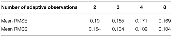
Table 3. The mean RMSE and RMSS using PE with different number of adaptive observations.

4. Conclusions

In this article, a new method is developed to use different dataset to perform state estimation and parameter estimation in the ensemble-based data assimilation. This method aims to cope with a major challenge of parameter estimation when it applies to real models. It is well-acknowledged that the parameter estimation for general circulation models is typically performed with joint state and parameter estimation. The issue is that the parameters usually take globally uniform values, and the assimilation of an enormous number of observations (which is necessary for state estimation) may cause the accumulation of sampling errors, thus adjust the parameters incorrectly. This work uses a serial DA methods to perform joint SE and PE, which permits the use of different dataset in SE and PE stages. The idea of target observation is adopted to update the model parameters with some crucial observations. From the algorithm of EAKF, we have defined the total variance reduction from one observation to all the parameters, which can be used to measure the impact of one potential observation to the parameter ensemble. By selecting the observation with maximum TVR, the uncertainty of parameters can be reduced most considerably.

The twin experiments with a two-scale Lorenz-96 model shows the advantages of the newly developed method over PE with fixed observations. On one hand, parameter estimation can reduce the model errors due to the uncertainty in parameterization, thus provides analyses with smaller errors. On the other hand, adaptive observations are the most effective observations that could be assimilated to reduce parameter ensemble spread, which accelerates the PE procedure to find better parameters. In addition, the locations of adaptive observations are not only derived statistically, but also reflect some of the model dynamics, as Figure 4 indicates.

In this work, the proposed PE method is applied with a very simple toy model with a basic parameterization scheme. The form of parameterization scheme may have impact on PE results. However, the advantage of using adaptive observations over using fixed observation can also be guaranteed even though more parameters are involved.

Moreover, this work is motivated by our recent study, i.e., Shen and Tang (2022), in which the parameter estimation is performed with the Community Earth System Model (CESM). Excessive parameter correction due to very small parameter space is an urgent problem. In that work, the ASA method by Liu et al. (2014a) is used. However, we think the proposed PE method which picks a few adaptive observations for PE, could be another possible solution. The potential advantage of the proposed method over ASA is that it does not change the global-uniform nature of the parameters, and it also saves a lot of computational efforts. In our next work, we will perform this PE strategy in that model.

Data Availability Statement

The original contributions presented in the study are included in the article/supplementary material, further inquiries can be directed to the corresponding author/s.

Author Contributions

ZS contributed to the conception, coding, experiments, and writing of this manuscript. QZ contributed to the conception and proofreading of this manuscript. ZC contributed to writing and editing of this manuscript. All authors contributed to the article and approved the submitted version.

Funding

This work was supported by grants from the National Natural Science Foundation of China (42176003), the Fundamental Research Funds for the Central Universities (B210201022), the Jiangsu Provincial Innovation and Entrepreneurship Doctor Program (JSSCBS20210252), and the Natural Science Foundation of Zhejiang Province grants (LQ18A010003).

Conflict of Interest

QZ is employed by Hangzhou Environmental Protection Science Research Design Co. Ltd.

The remaining authors declare that the research was conducted in the absence of any commercial or financial relationships that could be construed as a potential conflict of interest.

Publisher's Note

All claims expressed in this article are solely those of the authors and do not necessarily represent those of their affiliated organizations, or those of the publisher, the editors and the reviewers. Any product that may be evaluated in this article, or claim that may be made by its manufacturer, is not guaranteed or endorsed by the publisher.

Acknowledgments

We thank reviewers for the comments.

References

Aksoy, A., Zhang, F., and Nielsen-Gammon, J. W. (2006). Ensemble-based simultaneous state and parameter estimation with mm5. Geophys. Res. Lett. 33, L12801. doi: 10.1029/2006GL026186

CrossRef Full Text | Google Scholar

Anderson, J. L. (2001). An ensemble adjustment kalman filter for data assimilation. Month Weather Rev. 129, 2884–2903. doi: 10.1175/1520-0493(2001)129<2884:AEAKFF>2.0.CO;2

CrossRef Full Text | Google Scholar

Anderson, J. L. (2003). A local least squares framework for ensemble filtering. Month Weather Rev. 131, 634–642. doi: 10.1175/1520-0493(2003)131<0634:ALLSFF>2.0.CO;2

CrossRef Full Text | Google Scholar

Anderson, J. L. (2009a). Ensemble kalman filters for large geophysical applications. IEEE Control Syst. 29, 66–82. doi: 10.1109/MCS.2009.932222

CrossRef Full Text | Google Scholar

Anderson, J. L. (2009b). Spatially and temporally varying adaptive covariance inflation for ensemble filters. Tellus A 61, 72–83. doi: 10.1111/j.1600-0870.2008.00361.x

CrossRef Full Text | Google Scholar

Bellsky, T., Kostelich, E. J., and Mahalov, A. (2014). Kalman filter data assimilation: targeting observations and parameter estimation. Chaos Interdiscipl. J. Nonlin. Sci. 24, 024406. doi: 10.1063/1.4871916

PubMed Abstract | CrossRef Full Text | Google Scholar

Bergot, T. (2010). Adaptive observations during fastex: a systematic survey of upstream flights. Quart. J. R. Meteorol. Soc. 125, 3271–3298. doi: 10.1002/qj.49712556108

CrossRef Full Text | Google Scholar

Bishop, C. H., and Toth, Z. (1998). Ensemble transformation and adaptive observations. J.atmos 56, 1748–1765.

Duan, W., and Zhou, F. (2013). Nonlinear forcing singular vector of a two-dimensional quasi-geostrophic model. Tellus 65, 18452. doi: 10.3402/tellusa.v65i0.18452

CrossRef Full Text | Google Scholar

Emanuel, K., Raymond, D., Betts, A., Bosart, L., and Thorpe, A. (1995). Report of the first prospectus development team of the u.s. weather research program to noaa and the nsf. Bull. Am. Meteorol. Soc. 76, 1194–1208.

Furue, R., Jia, Y., McCreary, J. P., Schneider, N., Richards, K. J., Müller, P., et al. (2015). Impacts of regional mixing on the temperature structure of the equatorial pacific ocean. part 1: vertically uniform vertical diffusion. Ocean Modell. 91, 91–111.

Gaspari, G., and Cohn, S. (1999). Construction of correlation functions in two and three dimensions. Quart. J. R. Meteorol. Soc. 125, 723–757. doi: 10.1016/j.ocemod.2014.10.002

CrossRef Full Text | Google Scholar

Gharamti, M. E., Marzouk, Y. M., Huan, X., and Hoteit, I. (2015). “A greedy approach for placement of subsurface aquifer wells in an ensemble filtering framework,” in Dynamic Data-Driven Environmental Systems Science, eds S. Ravela and A. Sandu (Cham: Springer).

Huan, X., and Marzouk, Y. M. (2013). Simulation-based optimal bayesian experimental design for nonlinear systems. J. Comput. Phys. 232, 288–317. doi: 10.1016/j.jcp.2012.08.013

CrossRef Full Text | Google Scholar

Hunt, B. R., Kostelich, E. J., and Szunyogh, I. (2007). Efficient data assimilation for spatiotemporal chaos: a local ensemble transform kalman filter. Phys. D Nonlin. Phenomena 230. 112–126. doi: 10.1016/j.physd.2006.11.008

CrossRef Full Text | Google Scholar

Koyama, H., and Watanabe, M. (2010). Reducing forecast errors due to model imperfections using ensemble kalman filtering. Month. Weather Rev. 138, 3316–3332. doi: 10.1175/2010MWR3067.1

CrossRef Full Text | Google Scholar

Li, S., Zhang, S., Liu, Z., Lu, L., Zhu, J., Zhang, X., et al. (2018). Estimating convection parameters in the gfdl cm2.1 model using ensemble data assimilation. J. Adv. Model. Earth Syst. 10, 989–1010. doi: 10.1002/2017MS001222

CrossRef Full Text | Google Scholar

Liu, Y., Liu, Z., and Zhang, S. (2014a). Ensemble-based parameter estimation in a coupled gcm using the adaptive spatial average method*. J. Clim. 27, 4002–4014. doi: 10.1175/JCLI-D-13-00091.1

CrossRef Full Text | Google Scholar

Liu, Y., Liu, Z., Zhang, S., Jacob, R., Lu, F., Rong, X., and Wu, S. (2014b). Ensemble-based parameter estimation in a coupled general circulation model. J. Clim. 27, 7151–7162. doi: 10.1175/JCLI-D-13-00406.1

CrossRef Full Text | Google Scholar

Lorenz, E. (1996). “Predictability-a problem partly solved,” in Proc Seminar on Predictability (Reading: ECMWF).

Mu, M., Duan, W. S., and Wang, B. (2003). Conditional nonlinear optimal perturbation and its applications. Nonlin. Process. Geophys. 10, 493–501. doi: 10.5194/npg-10-493-2003

CrossRef Full Text | Google Scholar

Palmer, T. N., Gelaro, R., Barkmeijer, J., and Buizza, R. (1998). Singular vectors, metrics, and adaptive observations. J. Atmosph. Ences 55, 633–653.

Pu, Z. X., and Kalnay, E. (2010). Targeting observations with the quasi-inverse linear and adjoint ncep global models: performance during fastex. Quart. J. R. Meteorol. Soc. 125, 3329–3337. doi: 10.1002/qj.49712556110

CrossRef Full Text | Google Scholar

Sakov, P., and Oke, P. R. (2008). Objective array design: Application to the tropical indian ocean. J. Atmosph. Ocean. Technol. 25, 794–807. doi: 10.1175/2007JTECHO553.1

CrossRef Full Text | Google Scholar

Shen, Z., and Tang, Y. (2022). A two-stage inflation method in parameter estimation to compensate for constant parameter evolution in community earth system model. Acta Oceanologica Sinica 41, 12. doi: 10.1007/s13131-021-1856-5

CrossRef Full Text | Google Scholar

Tong, M., and Xue, M. (2008). Simultaneous estimation of microphysical parameters and atmospheric state with simulated radar data and ensemble square root kalman filter. part i: Sensitivity analysis and parameter identifiability. Month. Weather Rev. 136, 1630–1648. doi: 10.1175/2007MWR2070.1

CrossRef Full Text | Google Scholar

Torn, R. D., and Hakim, G. J (2008). Ensemble-based sensitivity analysis. Month. Weather Rev. 136, 663–677. doi: 10.1175/2007MWR2132.1

CrossRef Full Text | Google Scholar

Toth, Z., and Kalnay, E. (1997). Ensemble forecasting at ncep and the breeding method. Month. Weather Rev. 125, 3297–3319.

Whitaker, J. S., Hamill, T. M., Wei, X., Song, Y., and Toth, Z. (2008). Ensemble data assimilation with the ncep global forecast system. Month. Weather Rev. 136, 463–482. doi: 10.1175/2007MWR2018.1

PubMed Abstract | CrossRef Full Text | Google Scholar

Wilks, D. S. (2005). Effects of stochastic parametrizations in the lorenz '96 system. Quart. J. R. Meteorol. Soc. 131, 389–407. doi: 10.1256/qj.04.03

CrossRef Full Text | Google Scholar

Wu, X., Zhang, S., Liu, Z., Rosati, A., and Delworth, T. L. (2013). A study of impact of the geographic dependence of observing system on parameter estimation with an intermediate coupled model. Clim. Dyn. 40, 1789–1798. doi: 10.1007/s00382-012-1385-1

CrossRef Full Text | Google Scholar

Wu, Y., Shen, Z., and Tang, Y. (2020). A flow-dependent targeted observation method for ensemble kalman filter assimilation systems. Earth Space Sci. 7, e01149. doi: 10.1029/2020EA001149

CrossRef Full Text | Google Scholar

Zhang, S., Liu, Z., Rosati, A., and Delworth, T. (2012). A study of enhancive parameter correction with coupled data assimilation for climate estimation and prediction using a simple coupled model. Tellus A 64, 10963. doi: 10.3402/tellusa.v64i0.10963

CrossRef Full Text | Google Scholar

Zhang, S., Liu, Z., Zhang, X., Wu, X., and Deng, X. (2020). Coupled data assimilation and parameter estimation in coupled ocean-atmosphere models: a review. Clim. Dyn. 9, 5127–5144. doi: 10.1007/s00382-020-05275-6

CrossRef Full Text | Google Scholar