A novel adaptive Gaussian sum cubature Kalman filter with time-varying non-Gaussian noise for GNSS/SINS tightly coupled integrated navigation system

The Gaussian sum cubature Kalman filter (GSCKF) based on Gaussian mixture model (GMM) is a critical nonlinear non-Gaussian filter for data fusion of global navigation satellite system/strapdown inertial navigation systems (GNSS/SINS) tightly coupled integrated navigation system. However, the stochastic model of non-Gaussian noise in practical operating environments is not static, but rather time-varying. So if the GMM of GSCKF cannot be adjusted adaptively, it will lead to a decrease in estimation accuracy. To address this issue, we propose a novel adaptive GSCKF (AGSCKF) based on the dynamic adjustment of GMM. By analyzing the impact of GMM displacement parameter on the fitting accuracy of non-Gaussian noise, a novel algorithm for GMM displacement parameter adaptive adjustment is proposed using a cost function. Then this novel algorithm is applied to overcome the limitations of GSCKF under time-varying non-Gaussian noise environment, thereby improving the filtering performance. The simulation and experimental results indicate that the proposed AGSCKF exhibits significant advantage in changeable environments affected by time-varying non-Gaussian noise, which is applied to GNSS/SINS tightly coupled integrated navigation system data fusion can improve estimation accuracy and adaptability without sacrificing significant computational complexity.

1 Introduction

The global navigation satellite system and strapdown inertial navigation system (GNSS/SINS) tightly coupled integrated navigation system data fusion is one of the key technologies in many fields, including unmanned aerial vehicles (UAVs), which enables precise navigation, guidance, and control capabilities (Grewal et al., 2020; Gyagenda et al., 2022; Boguspayev et al., 2023). The mathematical model for GNSS/SINS tightly coupled integrated navigation system data fusion is inherently nonlinear, and despite advances in navigation technology, its nonlinear characteristics cannot be eliminated. Therefore, the nonlinear filter remains a crucial technique in the field of GNSS/SINS tightly coupled integrated navigation system data fusion for UAVs (Groves, 2008; Li and Chen, 2022; Xiao et al., 2024).

1.1 Nonlinear filter

Extended Kalman filter (EKF) is a widely used nonlinear filter for GNSS/SINS tightly coupled integrated navigation systems data fusion, but its engineering application is limited by linearization errors and complex updating processes of Jacobian matrix (Wang et al., 2018). Thus, Unscented Kalman filter (UKF) is proposed to approximate the state estimation and its covariance through a set of sampling points by unscented transforms (UT). Compared to EKF, UKF does not require updating Jacobian matrix, and its accuracy can reach second-order Taylor series expansion or even higher. However, the parameters of UKF do not have deterministic values, and the computation increases dramatically with the increase of the dimension of state estimation (Rhudy et al., 2011; Hu et al., 2020). Quadrature Kalman filter (QKF) using Gaussian Hermitian quadrature rule can achieve high estimation accuracy. But as the number of state parameters increases, the required quadrature points will exponentially increase, resulting in that the computational complexity of QKF is higher than that of EKF and UKF (Monfort et al., 2015). To address the dimensionality curse in QKF, researchers have devised cubature Kalman Filter (CKF). Within the CKF framework, the utilization of the third-order spherical cubature rule not only possesses a more rigorous mathematical foundation compared to the UT employed in UKF, but also demonstrates a reduction in computational resources and an increase in computational efficiency during state estimation under comparable conditions, as compared to both UKF and QKF. Additionally, by integrating a square-root filtering approach, CKF exhibits superior numerical stability when confronted with nonlinear challenges, in contrast to the UKF. Currently, CKF has been widely used in fields such as navigation positioning, target tracking, and guidance and control system due to its advantages of superior estimation accuracy, remarkable numerical stability, and minimal computational requirements (Arasaratnam and Haykin, 2009; Sindhuja et al., 2023). And yet CKF assumes that the random model in the filter is white Gaussian noise. In practical application, it is common for the random model to deviate from the assumption of white Gaussian noise, which inevitably affects the accuracy of filtering estimation (Sun et al., 2022; Tang et al., 2023; Wang et al., 2023). Therefore, mitigating the impact of non-Gaussian noise on the estimation accuracy of CKF has been a prominent research topic in the field of GNSS/SINS tightly coupled integrated navigation data fusion.

1.2 Mproved cubature Kalman filter

In recent years, various optimized algorithms for CKF have been proposed to address the issue of non-Gaussian noise in states estimation. A strong tracking CKF with multiple sub-optimal fading factor is introduced to tackle the discrepancy between theoretical and practical models of measurement noise in GNSS/SINS tightly coupled integrated navigation systems, which significantly enhances the accuracy of navigation estimation (Huang et al., 2016). Furthermore, a robust CKF based on M-estimation is presented, which can reduce the impact of non-Gaussian measurement noise interference. This filter redefines the innovation sequence using the M-estimate of Huber’s equivalent weight function, enhancing the robustness of the GNSS/SINS tightly coupled integrated navigation system data fusion (Wang et al., 2020). Additionally, an adaptive CKF based on Mahalanobis distance is designed to address the unknown noise statistics. By employing the Mahalanobis distance of innovations to determine the random model of filter, this filter improves the positioning accuracy of GNSS/SINS tightly coupled integrated navigation systems (Zhang et al., 2021). However, these above optimized algorithms for CKF approximate the true distribution of non-Gaussian through the Gaussian distribution approximation method with a larger variance, which may result in inaccurate estimated variance for state estimation (Legin et al., 2023; Dong et al., 2023).

Lately, the Gaussian mixture model (GMM) derived from the multimodal approximation method has emerged as a promising approach to solve non-Gaussian noise problems. Compared to the Gaussian distribution approximation method with a larger variance, the GMM offers higher accuracy in this regard (Alspach and Sorenson, 1972; George et al., 2022). By decomposing the probability density function (PDF) of non-Gaussian noise into multiple Gaussian components using GMM, Gauss-Hermite sum filter can be derived. Combining GMM with CKF yields the Gaussian sum CKF (GSCKF), which has been applied to GNSS/SINS tightly coupled integrated navigation data fusion, thereby contributing to improved navigation positioning accuracy (Bai et al., 2022). Since 2023, numerous improved algorithms for GSCKF have emerged in rapid succession, finding their applications within the domain of non-Gaussian nonlinear systems. These refined algorithms encompass: Credible GSCKF, Observability-Based GSCKF, quaternion constrained GSCKF, and so on (Ge et al., 2024; Jiang et al., 2024; Dai et al., 2024; Li et al., 2020). However, due to the non-stationary nature of practical operation environments of GNSS/SINS tightly coupled integrated navigation systems, the statistical characteristics of non-Gaussian noise also change over time (Zhou et al., 2024; Lin et al., 2023; Chen et al., 2023). Although the above research has to some extent improved the estimation accuracy of GNSS/SINS tightly coupled integrated navigation systems data fusion using GSCKF affected by non-Gaussian noises, the GMM modeling parameters in GSCKF cannot change with the statistical characteristics of non-Gaussian noise, and this limitation will lead to a decrease in estimation accuracy, which may seriously cause divergence.

1.3 Motivation and contributions

The motivation for this study stems from the intricate and dynamic nature of practical operating environments in GNSS/SINS tightly coupled integrated navigation system. These environments introduce time-varying non-Gaussian noise characteristics that exhibit stochastic behavior. Consequently, the inability of the GMM employed within GSCKF to adapt dynamically results in a degradation of estimation accuracy. Addressing the challenges posed by such time-varying non-Gaussian noise is crucial for maintaining the performance of GSCKF. Therefore, inspired by the research in reference (George et al., 2022; Dai et al., 2024; Lin et al., 2023; Panda et al., 2024a; Panda et al., 2024b), we propose a novel Adaptive GSCKF(AGSCKF), specifically designed to mitigate the adverse effects of time-varying non-Gaussian noise, thereby enhancing the performance of GNSS/SINS tightly coupled integrated navigation system.

The contributions of this work are concisely summarized as follows.

1) A novel AGSCKF is proposed, building upon the framework of GSCKF. This filter specifically targets the statistical properties of time-varying non-Gaussian noise, mitigating the adverse effects on the estimation accuracy of GSCKF.

2) The innovation of AGSCKF lies in its integration of a cost function-based adaptation algorithm. This algorithm dynamically optimizes the displacement parameter of GMM in real-time, ensuring precise tracking of the statistical characteristics of time-varying non-Gaussian noise.

3) Simulation and experimental analyses have been conducted to demonstrate the superior performance of AGSCKF, particularly in enhancing the estimation accuracy and adaptability of the GNSS/SINS tightly coupled integrated navigation system in time-varying non-Gaussian noise scenarios.

Collectively, these contributions highlight the superior performance of AGSCKF compared to CKF and GSCKF in addressing data fusion for GNSS/SINS tightly coupled integrated navigation systems in challenging environments.

2 Background and problem formulation

2.1 Mathematical models for GNSS/SINS tightly coupled integrated navigation system

The GNSS/SINS tightly coupled integrated navigation system exhibits excellent navigation accuracy and robustness against interference. Nevertheless, in the presence of high maneuvering, conventional linearized models tend to compromise the accuracy of estimation, necessitating the nonlinear mathematical model (Groves, 2008). The nonlinear mathematical model for GNSS/SINS tightly coupled integrated navigation system includes the state-space model and the measurement model.

The state estimation ${\mathit{x}}_{k-1\left|k-1\right.}$ at epoch k-1 encompasses attitude, velocity, position, gyroscope drift, accelerometer drift, GNSS clock bias, and GNSS clock drift. The state-space model can be mathematically expressed by Equation 1.

${\mathit{x}}_{k\left|k-1\right.}=f\left({\mathit{x}}_{k-1\left|k-1\right.}\right)+{\mathit{g}}_k{\mathit{w}}_k(1)$

where $f\left(\cdot \right)$ is a nonlinear function, ${\mathit{g}}_k$ is the noise coefficient matrix, ${\mathit{w}}_k$ is the process noise, Assuming that ${\mathit{w}}_k$ is characterized as white Gaussian noise, it can be represented mathematically as ${\mathit{w}}_k\sim \left(0,{\mathit{Q}}_k\right)$.

The measurement model is expressed by Equation 2.

${\mathit{z}}_k=h\left({\mathit{x}}_{k\left|k-1\right.}\right)+{\mathit{v}}_k(2)$

where ${\mathit{z}}_k$ is the measurement composed of pseud-orange and pseud-orange rate corrected by satellite clock bias, ionospheric delay, and tropospheric delay. $h\left(\cdot \right)$ is a nonlinear function. ${\mathit{v}}_k$ is the measurement noise caused by GNSS receiver, multipath effects, and orbit prediction residuals. Since ${\mathit{v}}_k$ does not conform to white Gaussian noise, it is classified as non-Gaussian noise. Its distribution can be closely approximated by two Gaussian components (Bai et al., 2022).

$\mathit{P}\left({\mathit{v}}_k\right)=\left(1-\epsilon \right)\mathrm{N}\left({\mathit{v}}_k^A;{\mathit{\mu }}_k^A,{\mathit{R}}_k^A\right)+\epsilon \mathrm{N}\left({\mathit{v}}_k^B;{\mathit{\mu }}_k^B,{\mathit{R}}_k^B\right)(3)$

where $\mathrm{N}\left({\mathit{v}}_k^A;{\mathit{\mu }}_k^A,{\mathit{R}}_k^A\right)$ is the Gaussian component of mean ${\mathit{\mu }}_k^A$ and variance ${\mathit{R}}_k^A$ at epoch $k$, $\mathrm{N}\left({\mathit{v}}_k^B;{\mathit{\mu }}_k^B,{\mathit{R}}_k^B\right)$ denotes the Gaussian component of mean ${\mathit{\mu }}_k^B$ and variance ${\mathit{R}}_k^B$, and $\epsilon$ represents a factor with unmeasurable and time-varying characteristics, setting $\epsilon \in \left[0,1\right]$.

2.2 Cubature Kalman filter

CKF is a Gaussian filter that enables the approximation of the PDF of nonlinear functions through a set of cubature points. This approach avoids the need for linearization of the nonlinear function, thereby enhancing the accuracy and reliability of states estimation. By utilizing this method, the CKF offers significant advantages over traditional linearized filters in terms of its ability to handle non-linear systems with high dimensional states estimation. The specific implementation steps of CKF are as follows.

Step 1: Initialization.

Set ${\mathit{x}}_{0\left|0\right.}\sim \mathrm{N}\left({\mathit{x}}_{0\left|0\right.},{\mathit{P}}_{0\left|0\right.}\right)$, ${\mathit{x}}_{0\left|0\right.}=\mathrm{E}\left({\mathit{x}}_{0\left|0\right.}\right)$ and ${\mathit{S}}_{0\left|0\right.}=\text{chol}\left({\mathit{P}}_{0\left|0\right.}\right)$, where $\mathrm{E}\left(\cdot \right)$ is the expected value, $\text{chol}\left(\cdot \right)$ represents the Cholesky decomposition, and ${\mathit{P}}_{0\left|0\right.}={\mathit{S}}_{0\left|0\right.}{\mathit{S}}_{0\left|0\right.}^{\mathrm{T}}$.

Step 2: Calculate the sampling points.

Let state estimation at epoch $k-1$ expressed as ${\mathit{x}}_{k-1\left|k-1\right.}$, and its covariance is computed as

${\mathit{P}}_{k-1\left|k-1\right.}={\mathit{S}}_{k-1\left|k-1\right.}{\mathit{S}}_{k-1\left|k-1\right.}^{\mathrm{T}}(4)$

The third-order spherical phase diameter cubature rule is employed to generate a set of cubature points ${\mathit{\xi }}_c$

${\mathit{\xi }}_c=\sqrt{\frac{m}{2}}{\left\{\left(\begin{array}{l}1\\ ⋮\\ 0\end{array}\right),\cdots ,\left(\begin{array}{l}0\\ ⋮\\ 1\end{array}\right),\left(\begin{array}{l}-1\\ ⋮\\ 0\end{array}\right),\cdots ,\left(\begin{array}{l}0\\ ⋮\\ -1\end{array}\right)\right\}}_c(5)$

In Equation 5, ${\mathit{x}}_{c,k-1\left|k-1\right.}$ denotes the total number of cubature points, $c=1,2,\cdots m$, $m=2n$. ${\mathit{x}}_{c,k-1\left|k-1\right.}$ is the dimension of the state estimation. In other words, the total number of cubature points is twice the dimension ${\mathit{x}}_{c,k-1\left|k-1\right.}$ of the state estimation.

Step 3: Prediction.

The estimation of cubature points ${\mathit{\chi }}_{c,k-1\left|k-1\right.}$ and propagation cubature points ${\mathit{x}}_{c,k-1\left|k-1\right.}^{*}$ are calculated separately.

${\mathit{\chi }}_{c,k-1\left|k-1\right.}={\mathit{S}}_{k-1\left|k-1\right.}{\mathit{\xi }}_c+{\mathit{x}}_{k-1\left|k-1\right.}(6)$

${\mathit{x}}_{c,k\left|k-1\right.}^{*}=f\left({\mathit{\chi }}_{c,k-1\left|k-1\right.}\right)(7)$

Calculate the state prediction ${\mathit{x}}_{k\left|k\right.-1}$ and its covariance ${\mathit{P}}_{k\left|k-1\right.}$

${\mathit{x}}_{k\left|k\right.-1}=\frac{1}{m}{\displaystyle \sum _{c=1}^m}{\mathit{x}}_{c,k\left|k-1\right.}^{*}(8)$

${\mathit{P}}_{k\left|k-1\right.}=\frac{1}{m}{\displaystyle \sum _{c=1}^m}\left({\mathit{x}}_{c,k\left|k-1\right.}^{*}-{\mathit{\chi }}_{c,k-1\left|k-1\right.}\right){\left({\mathit{x}}_{c,k\left|k-1\right.}^{*}-{\mathit{\chi }}_{c,k-1\left|k-1\right.}\right)}^{\mathrm{T}}+{\mathit{Q}}_{k-1}(9)$

where ${\mathit{Q}}_{k-1}$ is the covariance of process noise.

Step 4: Update.

Calculate measurement prediction ${\mathit{z}}_{k\left|k-1\right.}$, its corresponding covariance ${\mathit{P}}_{zz,k\left|k-1\right.}$, and cross-covariance ${\mathit{P}}_{xz,k\left|k-1\right.}$, respectively.

${\mathit{z}}_{k\left|k-1\right.}=\frac{1}{m}{\displaystyle \sum _{c=1}^m}{\mathit{z}}_{c,k\left|k-1\right.}^{*}(10)$

${\mathit{P}}_{zz,k\left|k-1\right.}=\frac{1}{m}{\displaystyle \sum _{c=1}^m}\left({\mathit{z}}_{c,k\left|k-1\right.}^{*}-{\mathit{z}}_{k\left|k-1\right.}\right){\left({\mathit{z}}_{c,k\left|k-1\right.}^{*}-{\mathit{z}}_{k\left|k-1\right.}\right)}^{\mathrm{T}}+{\mathit{R}}_k(11)$

${\mathit{P}}_{xz,k\left|k-1\right.}=\frac{1}{m}{\displaystyle \sum _{c=1}^m}\left({\mathit{x}}_{c,k\left|k-1\right.}^{*}-{\mathit{\chi }}_{c,k-1\left|k-1\right.}\right){\left({\mathit{z}}_{c,k\left|k-1\right.}^{*}-{\mathit{z}}_{k\left|k-1\right.}\right)}^{\mathrm{T}}(12)$

where ${\mathit{z}}_{c,k\left|k-1\right.}^{*}=h\left({\mathit{x}}_{c,k\left|k-1\right.}\right)$, ${\mathit{x}}_{c,k\left|k-1\right.}={\mathit{S}}_{k\left|k-1\right.}{\mathit{\chi }}_c+{\mathit{x}}_{k\left|k-1\right.}$, ${\mathit{P}}_{k\left|k-1\right.}={\mathit{S}}_{k\left|k-1\right.}{\mathit{S}}_{k\left|k-1\right.}^{\mathrm{T}}$.

Update the filter gain ${\mathit{K}}_k$, state estimation ${\mathit{x}}_{k\left|k\right.}$, and its covariance ${\mathit{P}}_{k\left|k\right.}$ separately.

${\mathit{K}}_k={\mathit{P}}_{xz,k\left|k-1\right.}{\mathit{P}}_{zz,k\left|k-1\right.}^{-1}(13)$

${\mathit{x}}_{k\left|k\right.}={\mathit{x}}_{k\left|k-1\right.}+{\mathit{K}}_k\left({\mathit{z}}_k-{\mathit{z}}_{k\left|k-1\right.}\right)(14)$

${\mathit{P}}_{k\left|k\right.}={\mathit{P}}_{k\left|k-1\right.}-{\mathit{K}}_k{\mathit{P}}_{zz,k\left|k-1\right.}{\mathit{K}}_k^{\mathrm{T}}(15)$

2.3 Gaussian sum cubature Kalman filter

CKF is a nonlinear filter that assumes the random model is white Gaussian noise. However, in practical operating environments, the measurement noise encountered in GNSS/SINS tightly coupled integrated navigation systems exhibits non-Gaussian characteristics. Consequently, it becomes imperative to combine CKF with GMM to develop states estimation of the GSCKF. The GSCKF enables CKF to effectively address the challenges posed by non-Gaussian noise, thereby enhancing the accuracy and reliability of state estimation for GNSS/SINS tightly coupled integrated navigation systems data fusion.

The distribution of measurement noise is depicted as non-Gaussian noise in Equation 3. However, due to the unmeasurable and time-varying characteristics of the factor $\epsilon$, $\mathit{P}\left({\mathit{v}}_k\right)$ is often decomposed into two Gaussian distributions with equidistant distributions as illustrated below:

$\mathit{P}\left({\mathit{v}}_k\right)\approx 0.5\mathrm{N}\left({\mathit{v}}_k^1;{\mathit{\mu }}_k^1,{\mathit{R}}_k^1\right)+0.5\mathrm{N}\left({\mathit{v}}_k^2;{\mathit{\mu }}_k^2,{\mathit{R}}_k^2\right)(16)$

where $\mathrm{N}\left({\mathit{v}}_k^1;{\mathit{\mu }}_k^1,{\mathit{R}}_k^1\right)$ represents a Gaussian component characterized by its mean ${\mathit{\mu }}_k^1$ and variance ${\mathit{R}}_k^1$. Similarly, $\mathrm{N}\left({\mathit{v}}_k^2;{\mathit{\mu }}_k^2,{\mathit{R}}_k^2\right)$ denotes another Gaussian component defined by its mean ${\mathit{\mu }}_k^2$ and variance ${\mathit{R}}_k^2$.

$\left\{\begin{array}{l}{\mathit{\mu }}_k^1={\mathit{\mu }}_k+d\sqrt{\lambda }u\\ {\mathit{\mu }}_k^2={\mathit{\mu }}_k-d\sqrt{\lambda }u\\ {\mathit{R}}_k^1={\mathit{R}}_k^2={\mathit{R}}_k-d^2\lambda u{u}^{\mathrm{T}}\end{array}\right.(17)$

where $\lambda$ and $\mathit{u}$ correspond to the maximum eigenvalue and the corresponding eigenvector of ${\mathit{R}}_k$, respectively. $d$ is the GMM displacement parameter that influences the mean distance between the two Gaussian components, $d\in \left[0,1\right]$. In practical computations, $d$ is typically set to 0.5 (Sun et al., 2020; Yu et al., 2023). As depicted in Figure 1, the decomposition process of GMM is illustrated as below.

Figure 1

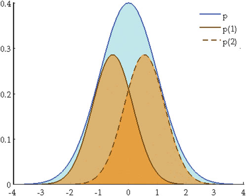
Figure 1. The decomposition process of GMM.

In Figure 1, the blue solid line $p$ represents the PDF of non-Gaussian noise, while the brown solid lines $p\left(1\right)$ and brown dotted lines $p\left(2\right)$ represent the two Gaussian components obtained through GMM decomposition respectively, with displacement parameter $d=0.5$. It can be seen that the probability density distribution after decomposition by GMM is close to the non-Gaussian noise in Equation 3. Therefore, GSCKF has better filtering performance than CKF owing to its accuracy random model under non-Gaussian noises scenarios.

The general implementation procedures of GSCKF can be described as follows. Firstly, based on GMM, the decomposition of non-Gaussian noise is performed using Equations 16, 17. Then, CKF is performed by employing Equations 4–15, and the state estimation of two components at the next epoch can be gotten separately. Finally, based on the weights of different components, a weighted combination is carried out to obtain the final state estimation and its covariance as outputs.

2.4 Flaws and shortcomings

The Allan variance analysis reveals that the measurement noise of GNSS/SINS tightly coupled integrated navigation systems is non-Gaussian in nature, rather than white Gaussian noise. Additionally, the mathematical statistical characteristics of non-Gaussian noise exhibit time-varying behavior due to changes in the practical operation environment over time (Tang et al., 2023; Zhang et al., 2020; Elmezayen and El-Rabbany, 2021; Taghizadeh and Safabakhsh, 2023). Although non-Gaussian noise can be approximated by Equation 17, the dynamic nature of the practical operation environment of GNSS/SINS tightly coupled integrated navigation systems introduces uncertainties in the factor, which makes the time-varying characteristics of $\mathit{P}\left(\mathit{v}\right)$. Therefore, it limits the optimality of the GMM displacement parameter when setting, as shown in Equation 17. In other words, if the GSCKF based on GMM with a fixed GMM displacement parameter is directly applied to GNSS/SINS tightly coupled integrated navigation systems data fusion, it may not effectively cope with time-varying non-Gaussian noise, resulting in random model mismatches, reduced estimation accuracy, and even divergence in severe cases.

3 Gaussian sum cubature Kalman filter with time-varying Non-Gaussian noise

To address the challenge of deteriorating estimation accuracy of GSCKF, where in the measurement noise is time-varying non-Gaussian noise, this section proposes a novel adaptive GSCKF (AGSCKF) based on the adaptively adjustment of the GMM displacement parameter. According to the impact analysis of GMM displacement parameter on the accuracy of GMM modeling, the AGSCKF employs an adaptive algorithm to select the optimal GMM displacement parameter between two Gaussian components to track changes in the statistical characteristics of non-Gaussian noise. As a result, the derivation of the AGSCKF for GNSS/SINS tightly coupled navigation system data fusion is achieved when measurement noise becomes time-varying non-Gaussian noise.

3.1 Analysis of the GMM displacement parameter on the accuracy of GMM modeling

The GSCKF decomposes non-Gaussian noise through GMM to obtain an approximate model by Equation 17, which makes the decomposed mixed model close to the non-Gaussian noise model in Equation 3. However, the time-varying $\epsilon$ in Equation 3 also introduces uncertainty for $\mathit{P}\left({\mathit{v}}_k\right)$ in Equation 17. And in the decomposition process of GMM, Equation 17 typically determines the GMM displacement parameter as $d=0.5$, which is not optimal. If $d>0.5$, the effect of $\epsilon \mathrm{N}\left({\mathit{v}}_k^B;{\mathit{\mu }}_k^B,{\mathit{R}}_k^B\right)$ is stronger than that of $\left(1-\epsilon \right)\mathrm{N}\left({\mathit{v}}_k^A;{\mathit{\mu }}_k^A,{\mathit{R}}_k^A\right)$; while $d>0.5$, the effect of $\epsilon \mathrm{N}\left({\mathit{v}}_k^B;{\mathit{\mu }}_k^B,{\mathit{R}}_k^B\right)$ is smaller than that of $\left(1-\epsilon \right)\mathrm{N}\left({\mathit{v}}_k^A;{\mathit{\mu }}_k^A,{\mathit{R}}_k^A\right)$. So, it is required that when non-Gaussian noise varies, the GMM displacement parameter can be adjusted adaptively.

In Figure 2, $p$ represents non-Gaussian noise in Equation 3, while $p\left(A\right)$ and $p\left(B\right)$ represent the two components in Equation 3. As shown in Figure 2A, when $d<0.5$, the GMM modeling result of Equation 17 is represented by the area enclosed by $p\left(1\right)$, $p\left(2\right)$ and the x-axis. The overlap between this area and the area enclosed by $p\left(A\right)$, $p\left(B\right)$ and the x-axis is the actual estimation result, denoted as M. The higher the overlap, the higher the estimation accuracy. On the other hand, when $d>0.5$, the actual estimation result, denoted as N in Figure 2A. Comparing M and N, it can be observed that the degree of overlap of M is lower than that of N, indicating that the estimation result shown in Figure 3D is better than that shown in Figure 3A.

Figure 2

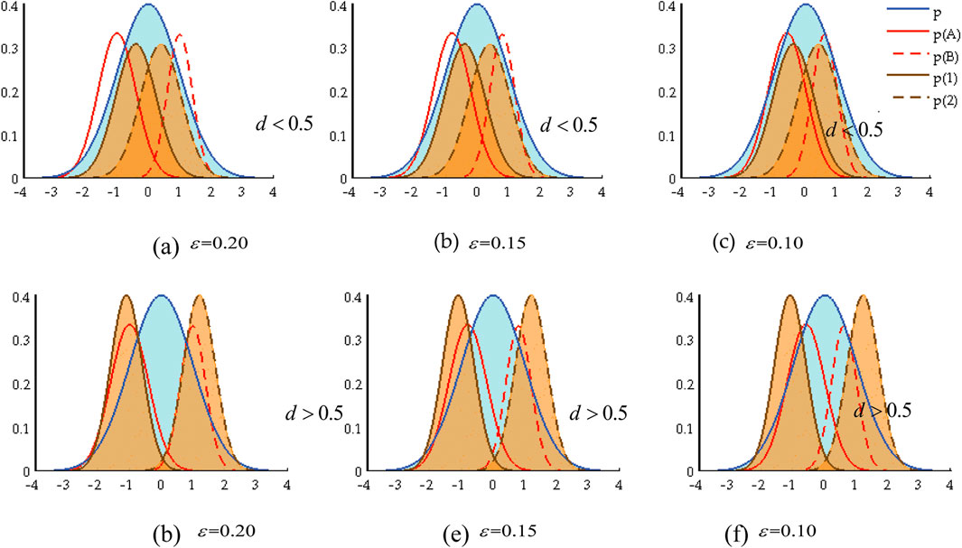
Figure 2. Relationship between the GMM displacement parameter and GMM modeling. (A) $\epsilon =0.20$ (B) $\epsilon =0.15$ (C) $\epsilon =0.10$. (D) $\epsilon =0.20$ (E) $\epsilon =0.15$ (F) $\epsilon =0.10$.

Figure 3

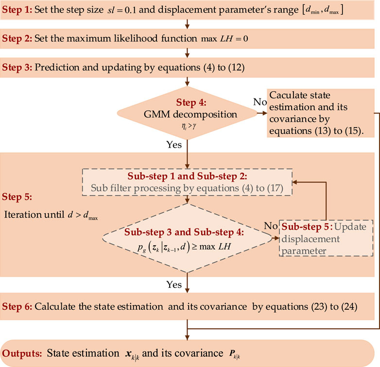
Figure 3. The flowchart of the proposed AGSCKF.

Further, as the effect of $\epsilon \mathrm{N}\left({\mathit{v}}_{\mathrm{B}};{\mathit{\mu }}_{\mathrm{B}},{\mathit{\Sigma }}_{\mathrm{B}}\right)$ weakens ($\epsilon$ changes from 0.20 to 0.10), the mean centers of $p\left(A\right)$ and $p\left(B\right)$ shift towards each other. The estimation result repressed as M′ when $d<0.5$ in Figure 3C, and the estimation result repressed as N′ when $d>0.5$ in Figure 3F. It is observed that the overlap degree of M′ is higher than that of N′, indicating that the estimation accuracy in Figure 3C is superior to that in Figure 3F when $d<0.5$.

This demonstrates that when non-Gaussian noise varies, adaptive adjustments in the GMM displacement parameter $d$ can effectively track the time-varying nature of non-Gaussian noise, resulting in a more reasonable GMM decomposition process and a closer fit to the actual non-Gaussian noise. By incorporating this approach into the GSCKF, more accurate stochastic models can be obtained, thereby enhancing the accuracy of GSCKF estimation.

3.2 Adaptive algorithm for the GMM displacement parameter

An adaptive algorithm is devised to address the real-time estimation challenge of the GMM displacement parameter under time-varying non-Gaussian noise condition. This algorithm employs the maximum value of the cost function as the optimal criterion and adaptively selects the optimal parameter within a specified range. The cost function is defined as follows:

$p\left({\mathit{z}}_k\left|{\mathit{z}}_{k-1},d\right.\right)=\frac{1}{\sqrt{2\pi {\sigma }^2}}\exp \left(-\frac{1}{2}{\left(\frac{{\mathit{z}}_k-{\mathit{z}}_{k\left|k-1\right.}}{\sigma }\right)}^2\right)(18)$

Subsequently, the corresponding value of the GMM displacement parameter $d$ within its range of variation $\left[d_{\min },d_{\max }\right]$ can be calculated. The GMM displacement parameter that corresponds to the maximum value $p\left(z_k\left|z_{k-1},d\right.\right)$ is identified as the optimal parameter value $\widehat{d}$ by Equation 19.

$\widehat{d}=\arg \max \widehat{p}\left(z_k\left|z_{k-1},d\right.\right)(19)$

where $d\in \left[d_{\min }{,d}_{\max }\right]$.

3.3 The process of AGSCKF

The proposed AGSCKF is derived by incorporating the adaptive algorithm for the GMM displacement into GSCKF. The specific implementation steps of the AGSCKF are as follows.

Step 1: Set the step size of displacement parameter’s changes $sl=0.1$ and displacement parameter’s range of variation $\left[d_{\min },d_{\max }\right]$.

The choice of step size has a significant impact on the accuracy of proposed AGSCKF. A smaller step size generally leads to higher accuracy, albeit at the cost of increased computational complexity.

Step 2: Let $d=d_{\min }$, and the maximum likelihood function is given by $\max LH=0$.

Step 3: The state prediction ${\mathit{x}}_{k\left|k-1,d\right.}$, measurement prediction ${\mathit{z}}_{k\left|k-1,d\right.}$, and its corresponding covariance ${\mathit{P}}_{k\left|k-1,d\right.}$, cross-covariance ${\mathit{P}}_{zz,k\left|k-1,d\right.}$ are computed utilizing Equations 4–12.

Step 4: To determine whether GMM decomposition is necessary, the nonlinearity $\eta$ is calculated by Equation 20.

$\eta =\frac{1}{2n}{\displaystyle \sum _{c=1}^{2n}}{\eta }_c(20)$

where ${\eta }_c=\frac{1}{2}{‖{\mathit{z}}_{c,k\left|k-1\right.}^{*}-h\left({\mathit{x}}_{k\left|k-1\right.}\right)‖}^2$. Set $\gamma$ is threshold. If ${\eta }_c>\gamma$, it is hypothesized that the high nonlinearity is exhibited in the presence of non-Gaussian noise, necessitating GMM decomposition. Consequently, the algorithm proceeds to the iteration of step 5. In contrast, if ${\eta }_c<\gamma$, GMM decomposition is not performed, the state estimation ${\mathit{x}}_{k\left|k\right.}$ and its corresponding covariance ${\mathit{P}}_{k\left|k\right.}$ at the subsequent epoch can be obtained using Equations 13–15.

Step 5: The following iteration (sub-step 1 to sub-step 5) is executed until $d>d_{\max }$.

Sub-step 1: The state prediction ${\mathit{x}}_{k\left|k-1,d\right.}^1$, the measurement prediction ${\mathit{z}}_{k\left|k-1,d\right.}^1$, and its corresponding covariance ${\mathit{P}}_{k\left|k-1,d\right.}^1$ and ${\mathit{P}}_{zz,k\left|k-1,d\right.}^1$ are calculated by Equations 4–15.

Sub-step 2: The state prediction ${\mathit{x}}_{k\left|k-1,d\right.}^2$, the measurement prediction ${\mathit{z}}_{k\left|k-1,d\right.}^2$, and its corresponding covariance ${\mathit{P}}_{k\left|k-1,d\right.}^2$ and ${\mathit{P}}_{zz,k\left|k-1,d\right.}^2$ are obtained by Equations 4–15.

Sub-step 3: In the presence of two Gaussian components, the cost function in Equation 18 is modified by Equation 21.

$\begin{array}{ll}\hfill p_g\left({\mathit{z}}_k\left|{\mathit{z}}_{k-1},d\right.\right)& =w^1\frac{1}{\sqrt{2\pi {\sigma }_1^2}}\exp \left(-\frac{1}{2}{\left(\frac{{\mathit{z}}_k-{\widehat{\mathit{z}}}_{k\left|k-1\right.}^1}{{\sigma }_1}\right)}^2\right)\hfill \\ \hfill & +w^2\frac{1}{\sqrt{2\pi {\sigma }_2^2}}\exp \left(-\frac{1}{2}{\left(\frac{{\mathit{z}}_k-{\widehat{\mathit{z}}}_{k\left|k-1\right.}^2}{{\sigma }_2}\right)}^2\right)\hfill \end{array}(21)$

where $w$ is the weight of components, and $\sigma$ is the covariance of measurement noise, superscript represent different components.

Sub-step 4: If $p_g\left({\mathit{z}}_k\left|{\mathit{z}}_{k-1},d\right.\right)\ge \max LH$, reset $\max LH=p_g\left({\mathit{z}}_k\left|{\mathit{z}}_{k-1},d\right.\right)$, and $\widehat{d}=d$.

Sub-step 5: Update the GMM displacement parameter $d$ by Equation 22.

$d=d+ST(22)$

Step 6: Based on the weights of components, calculate the state estimation ${\mathit{x}}_{k\left|k\right.}$ and its covariance ${\mathit{P}}_{k\left|k\right.}$ by Equations 23–26.

${\mathit{x}}_{k\left|k\right.}={\mathit{x}}_{k\left|k,\widehat{d}\right.}={\displaystyle \sum _{g=1}^2}{w}_k^{g,\widehat{d}}{\mathit{x}}_{k\left|k\right.}^g(23)$

${\mathit{P}}_{k\left|k\right.}={\mathit{P}}_{k\left|k,\widehat{d}\right.}={\displaystyle \sum _{g=1}^2}{w}_k^{g,\widehat{d}}\left[{\mathit{P}}_{k\left|k\right.}^g+\left({\mathit{x}}_{k\left|k\right.}^g-{\mathit{x}}_{k\left|k\right.}\right){\left({\mathit{x}}_{k\left|k\right.}^g-{\mathit{x}}_{k\left|k\right.}\right)}^{\mathrm{T}}\right](24)$

${\omega }_k^i={\omega }_{k-1}^i{\mathit{\beta }}_k^i/{\displaystyle \sum _{i=1}^2}{\omega }_{k-1}^i{\mathit{\beta }}_k^i(25)$

${\mathit{\beta }}_k^i\approx \mathrm{N}\left({\mathit{L}}_k-{\mathit{A}}_k{\overline{\mathit{X}}}_k,{\mathit{A}}_k{\mathit{\Sigma }}_{{\overline{X}}_k}{\mathit{A}}_k^{\mathrm{T}}+{\mathit{\Sigma }}_k^i\right)(26)$

Through the aforementioned calculation procedures, it becomes evident that the GMM displacement parameter can be adaptively adjusted, thereby bringing the non-Gaussian noise model shown in Equation 17 closer to that shown in Equation 3. This approach effectively addresses the limitations of GMM modeling inherent in the GSCKF. Consequently, the AGSCKF proposed in this section is theoretically expected to exhibit superior estimation accuracy compared to the GSCKF. The flowchart for the proposed AGSCKF is illustrated in Figure 3.

4 Performance evaluation and discussions

The proposed AGSCKF has been thoroughly assessed through simulations and experiments for GNSS/SINS tightly coupled integrated navigation system data fusion. In this section, the comparison and analysis of the proposed AGSCKF with CKF and GSCKF are discussed.

4.1 Simulations and analysis

The proposed AGSCKF is assessed for the data fusion of an UAV utilizing a GNSS/SINS tightly coupled integrated navigation system. The simulate trajectory of UAV flight, which includes various maneuvering states such as climbing, level flight, turning, and descending, is depicted in Figure 4. The initial attitude of UAV is all 0° in pitch, row and yaw respectively; the initial velocities are set as 0 m/s, 120 m/s and 0 m/s in the east, north and up respectively; the initial position is set as 110.20°, 34.00° and 2,000 m in longitude, latitude and altitude respectively. The simulated sensor’s parameters for the GNSS/SINS tightly coupled integrated navigation system are listed in Table 1. The GNSS measurement utilized in the simulation was derived from satellite constellations and epoch information obtained on 28 July 2023. Simulation duration is 1,000 s. Computer utilized in simulations encompasses an Intel Core i7-12700 CPU, 128 GB DDR4 memory, and Matlab R2020b software.

Figure 4

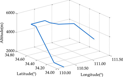
Figure 4. UAV flight trajectory.

Table 1

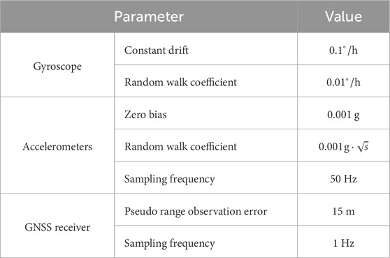
Table 1. Sensor’s parameters.

The initial parameters for three different algorithms (CKF, GSCKF and AGSCKF) are given in Table 2. The measurement non-Gaussian noise is generated by Equation 27.

$p\left({\mathit{v}}_k\right)\approx 0.9N\left(0,{\mathit{\Sigma }}_{\mathrm{A}}\right)+0.1N\left(0.5,{\mathit{\Sigma }}_{\mathrm{B}}\right)(27)$

where ${\mathit{\Sigma }}_{\mathrm{A}}=3{\mathit{\Sigma }}_{\mathrm{B}}=\text{diag}\left(0.3^2\cdots 0.3^2\right)$. In order to evaluate the performance of three different algorithms in terms of time-varying non-Gaussian noise, two different changes were implemented to the measurement non-Gaussian noise, respectively. During the epoch period from 401 s to 500 s and the epoch period from 601 s to 800 s, the measurement non-Gaussian noise is generated by Equation 28.

$p\left({\mathit{v}}_k\right)\approx 0.7N\left(0,{\mathit{\Sigma }}_{\mathrm{A}}\right)+0.3N\left(0.5,{\mathit{\Sigma }}_{\mathrm{B}}\right)(28)$

where ${\mathit{\Sigma }}_{\mathrm{A}}=3{\mathit{\Sigma }}_{\mathrm{B}}=\text{diag}\left(0.5^2\cdots 0.5^2\right)$.

Table 2

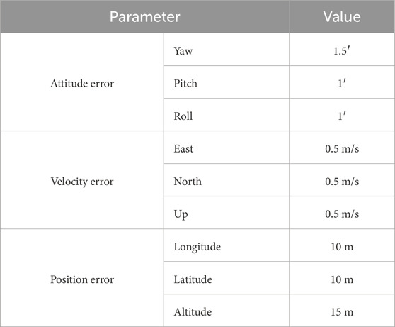
Table 2. Initial parameters for the algorithms.

The attitude error curves and positioning error curves of various algorithms (CKF, GSCKF, and AGSCKF) are illustrated in Figure 5. As can be observed from it, prior to the occurrence of changes for non-Gaussian noise statistical properties (0 s–400 s), the estimation error of CKF is highest of the three, while the estimation accuracies of GSCKF and AGSCKF are nearly equal and superior to that of CKF. This phenomenon can be attributed to the fact that GSCKF and AGSCKF employ GMM to model non-Gaussian noise, thereby mitigating its impact on estimation accuracy and ensuring enhanced attitude and positioning accuracy of GNSS/SINS tightly coupled integrated navigation systems operating in non-Gaussian noise environments.

Figure 5

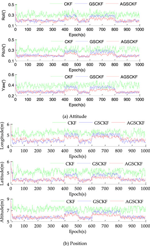
Figure 5. Estimation errors by the CKF, GSCKF and proposed AGSCKF for simulations. (A) Attitude (B) Position.

However, upon the occurrence of changes for non-Gaussian noise statistical properties (401 s–500 s, and 601 s–800 s), a significant increase in estimation error is observed for GSCKF as compared to AGSCKF. The discrepancy is caused by the change of non-Gaussian noise and the inability of the GMM displacement parameter of GSCKF to adapt accordingly, which leads to deterioration of estimation accuracy due to inaccurate GMM modeling for GSCKF. In contrast, the AGSCKF employs adaptive corrected GMM displacement parameter to achieve real-time tracking of time-varying non-Gaussian noise, thereby achieving more stable estimation performance than GSCKF.

In order to exemplify the impartiality of algorithm comparison, the root mean square error (RMSE) with 100 Monte-Carlo simulations is used to quantify the estimation accuracy of all the algorithms, which is defined by Equation 29.

$\text{RMSE}=\sqrt{\frac{1}{N}{\displaystyle \sum _{i=1}^I}{\left({\overline{\mathit{X}}}_i-{\mathit{X}}_i\right)}^2}(29)$

where $N$ is the total number of Monte Carlo simulations; ${\mathit{X}}_i$ is the reference; ${\overline{\mathit{X}}}_i$ is the state estimation. And the time consumption per epoch is calculated for the quantitative comparison of the computational complexity of various algorithms.

As shown in Table 3, the yaw is taken as an example. Prior to the occurrence of changes for non-Gaussian noise statistical properties (0 s–400 s), the estimation accuracy of GSCKF and AGSCKF are relatively close (0.317′ and 0.298′), both of which are higher than that of CKF (0.365′). When the first occurrence of changes for non-Gaussian noise statistical properties (401 s–500 s), AGSCKF achieves higher estimation accuracy due to real-time correction of GMM displacement parameter by AGSCKF. Compared to GSCKF and CKF, it has increased by 0.035′ and 0.080′, respectively. When the second occurrence of changes (601 s–800 s), the accuracy advantage of AGSCKF estimation is significant, with AGSCKF improving 0.034′ and 0.081′ compared to GSCKF and CKF, respectively.

Table 3

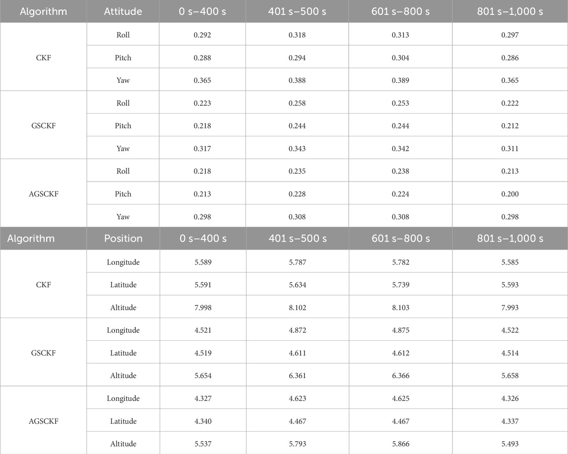
Table 3. (a): RMSEs of attitude errors (′). (b) RMSEs of position errors (′).

As depicted in Table 4 and Figure 6, it reveals that the changes of computation time for all three algorithms are relatively similar in all different epoch periods. Take epochs 601 s–800 s as example, the analysis of the average time spent per epoch reveals that CKF has the shortest computational time (5.84 ms) among all the algorithms. In contrast, the computational time of GSEKF is significantly larger than that of CKF by at least 135.66% times (7.92 ms). This is due to the complex computational process of GSCKF involved in distributed filtering and global point estimation at each epoch. Furthermore, the computational time of AGSCKF is at least 284.42% longer (16.61 ms) than that of CKF because AGSCKF needs to update the GMM displacement parameter by iteration.

Table 4

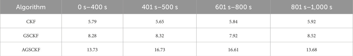
Table 4. The average time spent per epoch (ms).

Figure 6

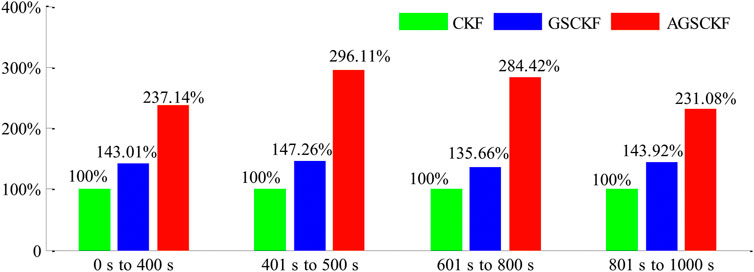
Figure 6. Relative computational complexity of the three different algorithms.

4.2 Experiments and analysis

This section presents the analysis and verification of the performance of the proposed AGSCKF through experiments. The experimental data was collected from a GNSS/SINS tightly coupled integrated navigation system mounted on UAVs. The experiment was conducted on 18 Oct 2023, at Zhengzhou, China. Table 5 shows the parameters of the SINS device and GNSS receiver in the GNSS/SINS tightly coupled integrated navigation system.

Table 5

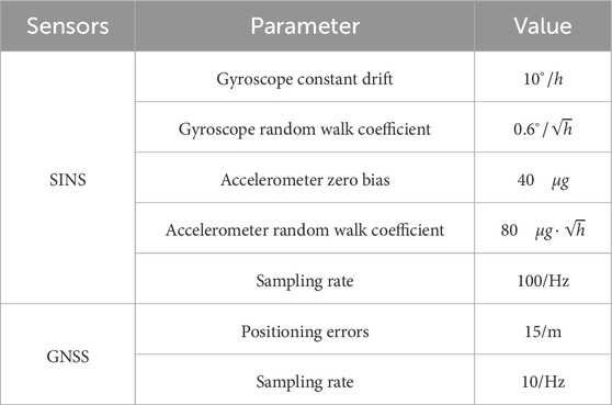
Table 5. Parameters of GNSS/SINS tightly coupled navigation system.

The initial position of the UAV was at latitude 34.654°, longitude 109.193°, and altitude 3,783 m, with initial velocities of 180 m/s, 60 m/s, and 40 m/s in the east, north, and up directions, respectively. The other initial parameters were consistent with those utilized in the simulations. A continuous data collection was conducted for a duration of 3,000 s, encompassing various maneuvering states such as climbing, level flight, turning, and descending. To ensure accurate results, a GNSS reference station was placed on the ground within a maximum distance of 20 km from the UAV. The differential data calculation result between the GNSS receiver on the UAV and the GNSS reference station served as the reference value. Subsequent post-processing yielded a differential positioning result with an accuracy better than 0.1 m. Three different algorithms same with simulation were employed for data fusion (CKF, GSCKF, and AGSCKF).

To assess the non-Gaussian and time-varying nature of GNSS measurement noise in experimental data, the statistical analysis was conducted on the pseudo-range noise of GNSS. The non-Gaussian nature of noise was measured using kurtosis. When $K=3$, the noise follows a Gaussian distribution; otherwise, it can be concluded that the noise does not follow a Gaussian distribution. When $K>3$, the noise obeys a super-Gaussian distribution or a thick-tailed distribution; when $K<3$, the noise obeys a sub-Gaussian distribution (Celikoglu and Tirnakli, 2018; Hatem et al., 2022). Table 6 presents the statistical characteristics of pseudo-range noise for the G22 satellite during different epoch periods.

Table 6

Table 6. Statistical characteristics analysis of G22 pseudo-range noise.

As depicted in Table 6, the kurtosis of the pseudo-range noise generated by the G22 satellite is noticeably less than 3 within the epoch intervals of [201,300] (s) and [1,301, 1,400] (s), indicating a negative kurtosis. This suggests that the G22 pseudo-range noise exhibits significant non-Gaussian characteristics. Conversely, the kurtosis of satellite’s pseudo-range noise within the epoch intervals of [801, 900] (s) and [1,101, 1,200] (s) are close to 3. As such, the G22 pseudo-range noise exhibits relatively weak non-Gaussian characteristics. This observation highlights the temporal variation in the statistical characteristics of non-Gaussian noise from measurement, which can be characterized as time-varying non-Gaussian noise.

The positioning error curves of different algorithms (CKF, GSCKF, and AGSCKF) during the epoch period of [0, 1,500] (s) are depicted in Figure 7. As observed from it, the range of changes for the CKF positioning error curve is significantly higher than that of GSCKF and AGSCKF. This can be attributed to the fact that CKF is unable to effectively counteract the influence of non-Gaussian noise, resulting in a larger positioning error. However, due to the use of GMM in GSCKF to accurately process the random model, the impact of non-Gaussian noise is mitigated. Consequently, the positioning accuracy of GSCKF has been enhanced. Furthermore, the maximum value of the positioning error curve variation range of AGSCKF is smaller than that of GSCKF. The main reason is that AGSCKF takes into account the time-varying non-Gaussian noise and employs the adaptive algorithm of GMM displacement parameter to improve the accuracy of GMM modeling, thereby minimizing the positioning error of AGSCKF.

Figure 7

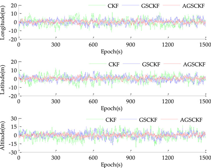
Figure 7. Position errors by CKF, GSCKF and proposed AGSCKF for experiment case.

To further validate the performance of the proposed AGSCKF, Table 7 presents a quantitative comparison of the RMSEs of different algorithms (CKF, GSCKF, and AGSCKF) for both 1,500 sets data and 3,000 sets data. As observed from it, an increase in navigation duration leads to a decrease in estimation accuracy for all algorithms. Specifically, when considering longitude positioning error as an example, CKF exhibits a reduction from 3.835 m to 4.067 m (about 5.70%), GSCKF shows a reduction from 3.245 m to 3.384 m (about 4.10%), and AGSCKF experiences a reduction from 2.854 m to 2.953 m (about 3.35%). It is evident that the estimation accuracy of AGSCKF consistently surpasses that of CKF and GSCKF. This highlights that AGSCKF not only possesses robust processing capabilities for time-varying non-Gaussian noise but also significantly enhances the GNSS/SINS tightly coupled integrated navigation positioning accuracy of UAVs in challenge environments. Furthermore, it maintains excellent stability of GNSS/SINS tightly coupled integrated positioning in long-sailing missions.

Table 7

Table 7. Comparison of estimation results with different datasets.

The computational complexity of AGSCKF is analyzed. It is observed that AGSCKF slightly increases the computation time per epoch, but does not result in a significant decrease in computational efficiency. This can be attributed to the fact that although AGSCKF requires iterative calculation of the GMM displacement parameter, relatively high-accuracy estimation can reduce the initial sensitivity of GMM and accelerate the convergence speed of GMM displacement parameter estimation.

In conclusion, the experiment confirms the same conclusion as the simulations, namely, that AGSCKF outperforms the other two algorithms (CKF and GSCKF) in terms of estimation accuracy and adaptability of GNSS/SINS tightly coupled integrated navigation data fusion.

5 Conclusion

The limitations of the GSCKF in the context of time-varying non-Gaussian noise of GNSS/SINS tightly coupled integrated navigation systems is analyzed theoretically. It is revealed that the GMM displacement parameter between Gaussian components significantly impact the accuracy of GMM fitting. To address this issue, a novel adaptive adjustment method for GMM displacement parameter is presented, which dynamically modifies this parameter through the cost function, thereby enhancing the rationality of the GMM decomposition process. This approach is incorporated into GSCKF to improve filtering accuracy, and effectively addresses the challenges posed by time-varying non-Gaussian noise, providing a viable solution to achieve high-accuracy estimation for GNSS/SINS tightly coupled integrated navigation systems operating in maneuvering states within challenging environments. Simulations and experiments demonstrate that the proposed AGSCKF enhances the estimation accuracy and adaptability of GSCKF in non-Gaussian noise condition, and exhibites superior stability in long-sailing missions. The research findings have significant implications for both nonlinear non-Gaussian filtering theory and GNSS/SINS tightly coupled integrated navigation systems data fusion algorithms for engineering applications.

While the proposed AGSCKF proves to be effective in modeling time-varying non-Gaussian noise in GNSS/SINS tightly coupled integrated navigation systems, it disregards the undefined noise scenarios, rendering the random model unable to adapt to the statistical characteristics of undefined noise. This limitation impairs the ability of AGSCKF proposed in this paper to effectively address undefined noise, potentially leading to a decline in estimation accuracy under severe conditions. So, the real-time dynamic GMM modeling techniques for undefined noise are very meaningful research points in the future.

Data availability statement

The raw data supporting the conclusions of this article will be made available by the authors, without undue reservation.

Author contributions

QD: Writing–original draft, Writing–review and editing. RW: Writing–review and editing. S-YH: Writing–review and editing. G-RX: Writing–original draft.

Funding

The author(s) declare that financial support was received for the research, authorship, and/or publication of this article. This research was funded by the following projects: The National Natural Science Foundation of China, grant number 42274045; the Henan Province Science and Technology Research Projects, grant number 242102241067; The Key Research Funding Projects for Higher Education Institutions in Henan Province, grant number 24A420003.

Conflict of interest

The authors declare that the research was conducted in the absence of any commercial or financial relationships that could be construed as a potential conflict of interest.

Publisher’s note

All claims expressed in this article are solely those of the authors and do not necessarily represent those of their affiliated organizations, or those of the publisher, the editors and the reviewers. Any product that may be evaluated in this article, or claim that may be made by its manufacturer, is not guaranteed or endorsed by the publisher.

References

Alspach, D., and Sorenson, H. (1972). Nonlinear bayesian estimation using Gaussian sum approximations. IEEE Trans. Automatic Control 17, 439–448. doi:10.1109/TAC.1972.1100034

CrossRef Full Text | Google Scholar

Arasaratnam, I., and Haykin, S. (2009). Cubature kalman filters. IEEE Trans. automatic control 54, 1254–1269. doi:10.1109/TAC.2009.2019800

CrossRef Full Text | Google Scholar

Bai, J. G., Ge, Q. B., Li, H., Xiao, J. M., and Wang, Y. L. (2022). Aircraft trajectory filtering method based on Gaussian-sum and maximum correntropy square-root cubature kalman filter. Cognitive Comput. Syst. 4, 205–217. doi:10.1049/ccs2.12049

CrossRef Full Text | Google Scholar

Boguspayev, N., Akhmedov, D., Raskaliyev, A., Kim, A., and Sukhenko, A. (2023). A comprehensive review of GNSS/INS integration techniques for land and air vehicle applications. Appl. Sci. 13 (8), 4819. doi:10.3390/APP13084819

CrossRef Full Text | Google Scholar

Celikoglu, A., and Tirnakli, U. (2018). Skewness and kurtosis analysis for non-Gaussian distributions. Phys. A Stat. Mech. its Appl. 499, 325–334. doi:10.1016/j.physa.2018.02.035

CrossRef Full Text | Google Scholar

Chen, H. K., Lu, T. D., Huang, J. H., He, X. X., Yu, K. G., Sun, X. W., et al. (2023). An improved VMD-LSTM model for time-varying GNSS time series prediction with temporally correlated noise. Remote Sens. 15 (14), 3694. doi:10.3390/RS15143694

CrossRef Full Text | Google Scholar

Dai, Q., Xiao, G. R., Zhou, G. H., Ye, Q., and Han, S. Y. (2024). A novel Gaussian sum quaternion constrained cubature Kalman filter algorithm for GNSS/SINS integrated attitude determination and positioning system. Front. Neurorobotics 18, 1374531. doi:10.3389/fnbot.2024.1374531

PubMed Abstract | CrossRef Full Text | Google Scholar

Dong, J. Q., Lian, Z. Z., Xu, J. C., and Yue, Z. (2023). UWB localization based on improved robust adaptive cubature kalman filter. Sensors 23 (5), 2669. doi:10.3390/S23052669

PubMed Abstract | CrossRef Full Text | Google Scholar

Elmezayen, A., and El-Rabbany, A. (2021). Real-time GNSS precise point positioning using improved robust adaptive kalman filter. Surv. Rev. 53, 528–542. doi:10.1080/00396265.2020.1846361

CrossRef Full Text | Google Scholar

Ge, Q. B., Cheng, Y., Yao, G., Chen, S., and Zhu, Y. (2024). Credible Gaussian sum cubature Kalman filter based on non-Gaussian characteristic analysis. Neurocomputing 565, 126922. doi:10.1016/J.NEUCOM.2023.126922

CrossRef Full Text | Google Scholar

George, S. M., Selvi, S. S., and Raol, J. R. (2022). Aircraft parameter estimation using Gaussian sum extended information filter with lyapunov stability analysis. Int. J. Veh. Struct. and Syst. 14, 540–545. doi:10.4273/IJVSS.14.4.23

CrossRef Full Text | Google Scholar

Grewal, M. S., Andrews, A. P., and Bartone, C. G. (2020). Global navigation satellite systems, inertial navigation, and integration. Hoboken, NJ, USA: John Wiley and Sons. doi:10.1002/9781119547860

CrossRef Full Text | Google Scholar

Groves, D. P. (2008). Principles of GNSS, inertial, and multisensor integrated navigation systems. London, England: Artech House, 7–20. doi:10.1017/s0373463313000672_1

CrossRef Full Text | Google Scholar

Gyagenda, N., Hatilima, J. V., Roth, H., and Zhmud, V. (2022). A review of GNSS-independent UAV navigation techniques. Robotics Aut. Syst. 152, 104069. doi:10.1016/J.ROBOT.2022.104069

CrossRef Full Text | Google Scholar

Hatem, G., Zeidan, J., Goossens, M., and Moreira, C. (2022). Normality testing methods and the importance of skewness and kurtosis in statistical analysis. BAU Journal-Science Technol. 3 (2), 7. doi:10.54729/KTPE9512

CrossRef Full Text | Google Scholar

Hu, G. G., Gao, B. B., Zhong, Y. M., and Gu, C. F. (2020). Unscented kalman filter with process noise covariance estimation for vehicular ins/gps integration system. Inf. Fusion 64, 194–204. doi:10.1016/j.inffus.2020.08.005

CrossRef Full Text | Google Scholar

Huang, W., Xie, H. S., Shen, C., and Li, J. P. (2016). A robust strong tracking cubature kalman filter for spacecraft attitude estimation with quaternion constraint. Acta Astronaut. 121, 153–163. doi:10.1016/j.actaastro.2016.01.009

CrossRef Full Text | Google Scholar

Jiang, H., Zhang, Y., Wang, X., and Cai, Y. (2024). Observability-based Gaussian sum cubature Kalman filter for three-dimensional target tracking using a single two-dimensional radar. Remote Sens. 16 (22), 4172. doi:10.3390/rs16224172

CrossRef Full Text | Google Scholar

Legin, R., Adam, A., Hezaveh, Y., and Perreault-Levasseur, L. (2023). Beyond Gaussian noise: a generalized approach to likelihood analysis with non-Gaussian noise. Astrophysical J. Lett. 949 (2), L41. doi:10.3847/2041-8213/ACD645

CrossRef Full Text | Google Scholar

Li, B. F., and Chen, G. E. (2022). Improving the combined GNSS/INS positioning by using tightly integrated RTK. GPS Solutions 26 (4), 144. doi:10.1007/S10291-022-01331-2

CrossRef Full Text | Google Scholar

Li, D. G., Wu, Y. Q., and Zhao, J. M. (2020). Novel hybrid algorithm of improved CKF and GRU for GPS/INS. IEEE Access 8, 202836–202847. doi:10.1109/ACCESS.2020.3035653

CrossRef Full Text | Google Scholar

Lin, X. Y., Liu, L. L., Dong, Y. Y., Chen, X. G., and Yang, H. L. (2023). Improved adaptive filtering algorithm for GNSS/SINS integrated navigation system. Geomatics Inf. Sci. Wuhan Univ. 48, 127–134. doi:10.13203/j.whugis20200436

CrossRef Full Text | Google Scholar

Monfort, A., Renne, J. P., and Roussellet, G. (2015). A quadratic Kalman filter. J. Econ. 187, 43–56. doi:10.1016/j.jeconom.2015.01.003

CrossRef Full Text | Google Scholar

Panda, A., Mahapatra, S., Ag, K. R., and Panda, R. C. (2024b). Lowering carbon emissions from a zinc oxide rotary kiln using event-scheduling observer-based economic model predictive controller. Chem. Eng. Res. Des. 207, 420–438. doi:10.1016/j.cherd.2024.06.017

CrossRef Full Text | Google Scholar

Panda, A., Thirunavukarasu, N., and Panda, R. C. (2024a). Predictive control scheme by integrating event-triggered mechanism and disturbance observer under actuator failure and sensor fault. Proc. Institution Mech. Eng. Part I J. Syst. Control Eng. 238 (4), 621–647. doi:10.1177/09596518231204725

CrossRef Full Text | Google Scholar

Rhudy, M., Gu, Y., Gross, J., and Napolitano, M. R. (2011). Sensitivity analysis of EKF and UKF in GPS/INS sensor fusion. AIAA guidance navigation and control conference. Portland, Oregon, USA. doi:10.2514/6.2011-6491

CrossRef Full Text | Google Scholar

Sindhuja, P. P., Panda, A., Velappan, V., and Panda, R. C. (2023). Disturbance-observer-based finite time sliding mode controller with unmatched uncertainties utilizing improved cubature Kalman filter. Trans. Inst. Meas. Control 45 (9), 1795–1812. doi:10.1177/01423312221140507

CrossRef Full Text | Google Scholar

Sun, B., Zhang, Z. W., Liu, S. C., Yan, X. B., and Yang, C. X. (2022). Integrated navigation algorithm based on multiple fading factors kalman filter. Sensors 22, 5081. doi:10.3390/S22145081

PubMed Abstract | CrossRef Full Text | Google Scholar

Sun, L. L., Cao, Y. H., Wu, W. H., and Liu, Y. T. (2020). A multi-target tracking algorithm based on Gaussian mixture model. J. Syst. Eng. Electron. 31, 482–487. doi:10.23919/jsee.2020.000020

CrossRef Full Text | Google Scholar

Taghizadeh, S., and Safabakhsh, R. (2023). Low-cost integrated INS/GNSS using adaptive H∞ cubature kalman filter. J. Navigation 76, 1–19. doi:10.1017/S0373463322000583

CrossRef Full Text | Google Scholar

Tang, J., Bian, H. W., Ma, H., and Wang, R. Y. (2023). Initialization of SINS/GNSS error covariance matrix based on error states correlation. IEEE Access 11, 94911–94917. doi:10.1109/ACCESS.2023.3293158

CrossRef Full Text | Google Scholar

Wang, G. C., Xu, X. S., and Zhang, T. (2020). M-M estimation-based robust cubature kalman filter for INS/GPS integrated navigation system. IEEE Trans. Instrum. Meas. 70, 1–11. doi:10.1109/TIM.2020.3021224

CrossRef Full Text | Google Scholar

Wang, J. W., Chen, X. Y., and Shi, C. F. (2023). A novel robust iterated CKF for GNSS/SINS integrated navigation applications. Eurasip J. Adv. Signal Process. 1, 83. doi:10.1186/S13634-023-01044-9

CrossRef Full Text | Google Scholar

Wang, M. S., Wu, W. Q., Zhou, P. Y., and He, X. F. (2018). State transformation extended Kalman filter for GPS/SINS tightly coupled integration. GPS Solutions 22, 112–12. doi:10.1007/s10291-018-0773-3

CrossRef Full Text | Google Scholar

Xiao, G. R., Yang, C., Wei, H. P., Xiao, Z. Y., Zhou, P. Y., Li, P. G., et al. (2024). PPP ambiguity resolution based on factor graph optimization. GPS solutions 28 (4), 178. doi:10.1007/s10291-024-01715-6

CrossRef Full Text | Google Scholar

Yu, B., Zhang, Y. Z., Xie, W. S., Zuo, W. J., Zhao, Y. M., and Wei, Y. L. (2023). A network traffic anomaly detection method based on Gaussian mixture model. Electronics 12 (6), 1397. doi:10.3390/ELECTRONICS12061397

CrossRef Full Text | Google Scholar

Zhang, B., Wang, X. D., Lu, H., Hao, Z. J., and Gu, C. C. (2021). Application of adaptive robust CKF in SINS/GPS initial alignment with large azimuth misalignment angle. Math. Problems Eng. 2021, 1–6. doi:10.1155/2021/7398706

CrossRef Full Text | Google Scholar

Zhang, Q., Niu, X. J., and Shi, C. (2020). Impact assessment of various IMU error sources on the relative accuracy of the GNSS/INS systems. IEEE Sensors J. 20, 5026–5038. doi:10.1109/jsen.2020.2966379

CrossRef Full Text | Google Scholar

Zhou, P., Xiao, G., and Du, L. (2024). Initial performance assessment of galileo high accuracy service with software-defined receiver. GPS solutions 28 (1), 2. doi:10.1007/s10291-023-01540-3

CrossRef Full Text | Google Scholar