 Belthasara Assan
- 1Department of Mathematics and Applied Mathematics, University of Johannesburg, Johannesburg, South Africa
- 2Institute of Applied Research and Technology, Emirates Aviation University, Dubai, United Arab Emirates
From the beginning of the outbreak of SARS-CoV-2 (COVID-19), South African data depicted seasonal transmission patterns, with infections rising in summer and winter every year. Seasonality, control measures, and the role of the environment are the most important factors in periodic epidemics. In this study, a deterministic model incorporating the influences of seasonality, vaccination, and the role of the environment is formulated to determine how these factors impact the epidemic. We analyzed the stability of the model, demonstrating that when R0 < 1, the disease-free equilibrium is globally symptomatically stable, whereas R0 > 1 indicates that the disease uniformly persists and at least one positive periodic solution exists. We demonstrate its application by using the data reported by the National Institute for Communicable Diseases. We fitted our mathematical model to the data from the third wave to the fifth wave and used a damping effect due to mandatory vaccination in the fifth wave. Our analytical and numerical results indicate that different efficacies for vaccination have a different influence on epidemic transmission at different seasonal periods. Our findings also indicate that as long as the coronavirus persists in the environment, the epidemic will continue to affect the human population and disease control should be geared toward the environment.
1. Introduction
The coronavirus disease (COVID-19) pandemic is now a worldwide epidemic that has been rapidly growing from the onset and is caused by the severe acute respiratory syndrome coronavirus 2 (SARS-CoV-2) which has a significant morbidity and mortality estimate of 0.5–2% of confirmed cases [1]. The world experienced its first zoonotic human coronavirus, in 2002, the severe acute respiratory syndrome coronavirus (SARS-CoV) spread to 37 countries in 2012, and the second is the Middle East respiratory syndrome coronavirus (MERS-CoV), also spread to 27 countries [2]. COVID-19 is currently recorded in 230 countries as of November 2022, with more than 638 million cases and 6.8 million deaths. South Africa was leading the African continent with over 4 million cases and 102, 000 thousand deaths.
Symptoms of COVID-19 infection include breathing difficulty, fever, fatigue, a dry cough, and in severe cases, bilateral lung infiltration and others also developed non-respiratory symptoms, including vomiting, diarrhea, and nausea [2–4] similar to the symptoms of SARS-CoV and MERS-CoV.
According to WHO [5], the COVID-19 virus is primarily transmitted between people through respiratory droplets and contact routes. Droplet transmission occurs when an infected person sings, breathes, sneezed, coughed, and has nasal discharge [6]. Transmission can also occur through fomites in the immediate environment around the infected person [7]. Therefore, the COVID-19 virus can be transmitted by direct contact with infected people and indirect contact with surfaces in the immediate environment or with objects used on or by the infected person [7].
In the analysis done by Kampf et al. [8] on 22 types of coronaviruses, it revealed that human coronaviruses such as severe acute respiratory syndrome (SARS) coronavirus, Middle East respiratory syndrome (MERS) coronavirus or endemic human coronaviruses (HCoV) could persist on inanimate surfaces such as metal, glass, or plastic for up to 9 days, and this gives evidence of the survival of the pathogens in the environment to increase risk of infection again. In Gralinski and Menachery [3], it was reported that samples taken from the Huanan Seafood Market, a live animal and seafood wholesale market in Wuhan, were positive for COVID-19, which suggested that pathogens could be transmitted through the environmental reservoir [9, 10]. COVID-19 has also been found in the stool of some infected individuals, which may contaminate the aquatic environment [2, 11].
Evidence suggested that infected humans continued to shed virus into the environment as long as they were infectious [12]. The European Congress of Clinical Microbiology and Infectious Diseases [13] reported a COVID-19 patient who tested positive for 505 days until death. Furthermore, a report by Spanish researchers [14] described a 52-year-old man who shed the virus after 189 days of chemotherapy and a 64-year-old man also continued to shed the virus for 169 days after being infected [15]. Rahmani et al. [16] examined the length of time in an infected person with SARS-CoV-2 continued to shed the virus. It was discovered that the typical person continues to shed the virus for a month. However, some individuals' bodies continued to discharge the virus for a long time.
López and Rodo [17], Liu et al. [18], and Wang et al. [19] reported that control measures were important factors in containing epidemics and reducing the transmission of the disease. During the early stages, different levels of control measures had different impacts on the transmission of COVID-19 [20–22]. Strict controls were by closing public facilities, and some mild control measures included maintaining social distancing, taking temperature measurements, and wearing masks. All these control measures were implemented from the first wave to the fourth wave of COVID-19 in South Africa since there were no pharmaceutical inventions. However, during those times, most developed mathematical models did not consider vaccinations [9, 23–25]. Recent mathematical models that have been developed include vaccination as a major control measure [26, 27].
Regardless of these control measures, seasonality is another important factor that influences epidemics. There has been much controversy regarding COVID-19, with questions over its transmission regarding seasonal patterns including other seasonal epidemics such as flu [9, 28–30]. Some studies have attempted to establish the relationship between COVID-19 and seasonality by varying meteorological factors [9]. In a study by Matson et al. [31] and Liu et al. [18], it pointed out that the stability of the virus in the air or on surfaces is quick to respond to environmental conditions, including humidity, temperature, sunlight, and more. The virus is more stable at low-temperature and low-humidity conditions, whereas warmer temperatures and higher humidity give it a half-life. Moreover, experimental data and regional analysis by Yao et al. [32] showed that COVID-19 in a high-temperature environment had a lower survival rate and infections declined in summer. At 4°, 22°, and 37°, SARS-CoV-2 can persist for 14, 7, and 1 day, respectively, under laboratory conditions. However, at 56°, it persistence reduce drastically to 10 min [18, 33]. In addition, Chin et al. [33] found that at 4° the virus was stable and inactive when increased to 70°. Confirmed cases of COVID-19 were found to be concentrated at an absolute humidity of 3 to 10g/m3 at air temperatures of 5 to 15° in Huang et al. [34]. The following study and experiment also confirmed with similar findings, SARS-CoV-2 can remain viable and infectious in aerosols for hours at room temperature 21°—23° and a fixed relative humidity of 65% [35]. Simulated sunlight can rapidly inactivate SARS-CoV-2 suspended in either simulated saliva or culture media and dried on stainless steel coupons [18, 36].
Many mathematical models have been developed since the appearance of COVID-19 disease. Most of these models are based on the significant role of human-to-human transmission as done by Chan et al. [37], Ojo et al. [23], and Babasola et al. [24]. However, several studies have given evidence of pathogen transmission through the environmental reservoir. Few mathematical models have been developed so far to consider the role of the human-to-environment transmission [9, 10, 38]. However, seasonal patterns expose the limitations of many recent COVID-19 models that do not incorporate seasonality. In this study, we consider South Africa, with two main climate seasons in a year. During these periods, there has always been a surge in infections. We present a mathematical model for COVID-19 that considers double periodic transmission pathways: human-to-human periodic transmission and periodic transmission through the environmental reservoir (human-to-environment). We divide our human population into five sub-populations: susceptible individuals, exposed individuals, asymptomatic individuals, symptomatic individuals, and recovered individuals. The transmission rate incorporates the influence of seasonality, control measures (vaccination), and the environment. We analyzed the basic reproduction number (using the next infection operator) and establish that it is a sharp threshold for the COVID-19 models with the periodic transmission. The analysis method for extinction and persistence results for periodic epidemic systems is inspired by the research done in Wang and Zhao [2]. We fit our mathematical model to data obtained from the National Institute for Communicable Diseases, South Africa [39], to estimate parameters and then simulate the efficacy driven by the vaccination parameter.
The study is organized as follows. In Section 2, we present the model and its properties. In Section 3, a detailed mathematical analysis is performed on the model developed. In Section 4, we explain numerical simulations, and conclude the study with some discussion and recommendations in Section 5.
2. Model formulation and properties
2.1. Model formulation
We define N(t) as the total human population at time t. The human population is divided into five classes: the susceptible class S(t), the exposed class E(t); those who have been exposed to the virus but have not yet been diagnosed as COVID-19 positive, the asymptomatic class Ia(t); people who have been diagnosed with COVID-19 but do not exhibit any clinical symptoms, the symptomatic individuals Is(t); people with clinical symptoms who have been diagnosed as COVID-19 positive and recovered class R(t); and people who have recovered from the virus. The human population has a natural mortality rate of μ. The total population is given as
Ce(t) is the pathogen concentration in the environment at a given time (t). The removal rate of the virus is σ. The environmental reservoir is defined in this study as fomites in the immediate environment around the infected person and sheddings by infected humans either through droplets or feces. The relationship between humans and the environment is represented in Figure 1.
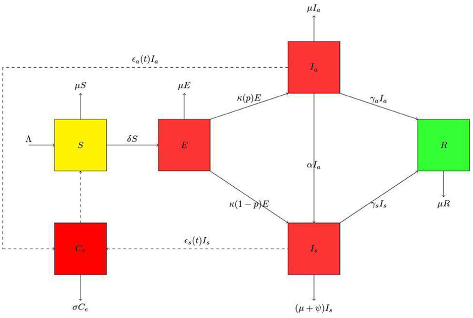
Figure 1. Schematic diagram for the presented model. The human population is divided into susceptible class (S), exposed class (E), asymptomatic class (Ia), symptomatic class (Is) and the recovered class (R). Thus, the population at any time t is N = S + E + Ia + Is + R. In the environmental population, Ce is the environmental pathogens. We have used the dashed lines with arrowheads to indicate contact and solid lines with arrowheads to indicate movement.
The dynamics of the susceptible population is given in Equation (2), Λ being the recruitment rate. The second term δ(t, Ia, Is, Ce) determines the rate of new infection, the parameter δ is the disease transmission rate and is time dependent.
where
The parameter β(t) is the effective contact rate of susceptible humans with the asymptomatic class Ia, symptomatic class Is, and the environment Ce, respectively. K50 gives the concentration of virus in the environment that yield 50% chance of infection with COVID-19. η measures the relative infectivity between Ia and Is, and it is measured between 0 ≤ η ≤ 1.
ˆβˉβ is the amplitude of the periodic oscillations when ˉβ=0 means there are no infections in the periodic function. Here, ˆβ is the baseline value or the time average, ω=3652=182.5 days since there are only two waves in a year and a time-varying vaccination parameter m(t), to formulate the influence of control measures. It gives the quantitative estimation of the control measure implemented in South Africa. We define our m(t)=e-mxtx, which falls between (0, 1], when m(t) = 1 then the epidemic spreads without any restrictions; however, m(t) can not be assumed to be one except when there are no any control measures, and when m(t) = 0, then there is no epidemic. mx controls the speed at which the vaccination reaches its maximum or minimum values, and we call it the vaccination efficacy in our study. Moreover, tx gives the start time of the vaccination.
For the exposed population, in Equation (4), the first term represents those who enter from the susceptible pool driven by the force of infection δ. The rate κ is the progression rate of exposed individuals to the asymptomatic and symptomatic classes.
The dynamics of the symptomatic individuals infected with COVID-19 is given in Equation (5). In the first term, p gives the proportion of humans that are moving from the exposed class to the asymptomatic class, α is the rate of transfer from the asymptomatic to the symptomatic class, and γa is the recovery rate for the asymptomatic class respectively.
The dynamics of the asymptomatic individuals infected with COVID-19 is given in Equation (6). In the third term, ψ is the disease-induced mortality rate and γs is the rate of recovery for symptomatic individuals.
The dynamics of the recovered individual are represented in Equation (7),
The environmental dynamics is given in Equation (8), where ϵa(t) is the shedding rate from the asymptomatic class, which is time-dependent, ϵs(t) is the shedding rate from the symptomatic class which is time-dependent, and the rate σ is is the removal of the virus from the environment, respectively. Here, ϵa(t) and ϵs(t) are given by
The amplitude of the periodic oscillations in ϵa, s(t) is given by ˆϵa,sˉϵa,s and when ˉϵa,s=0, no infections in the periodic function and baseline values or the time-average is ˆϵa,s. ω=3652=182.5 days since we have only two waves in a year.
We re-scale Equations (2)–(8), using the following substitutions:
The virus in the environment has a carrying capacity of Kce, Equations (2)–(8) changes into the following subsystems
where
We remove the fifth equation in Equation (10) since it is independent of the rest of the equations and rewrite the system as follows:
2.2. Model properties
The human population and environmental reservoir are differentiable and periodic in time with a common period ω.
To make biological sense, we assume that the functions δ and ζ satisfy the following conditions for all t ≥0:
•(P1) δ(t, 0, 0, 0) = ζ(t, 0, 0, 0) = 0, the disease-free equilibrium is unique and constant. Let E0 denote the disease-free equilibrium, which is given as
•(P2) The force of infection, δ(t, ia, is, x) ≥ 0. This property ensures we have a non-negative for all time.
•(P3)
The first set of equations in Property (13) ensures that the rate of new infection increases with both the infected human population and the pathogen concentration. The second set of equations in Property (14) ensures an increase in human infections and, therefore, a higher level of human contribution to the environmental virus, leading to a higher growth rate for the pathogens. The property (15) ensures that the rate of change of the pathogen concentration would be negatively related to itself [40].
•(P4) δ(t, ia, is, x) and ζ(t, ia, is, x) are both concave for any t ≥ 0. This property ensures that the second partial derivative is concave.
and is negative semidefinite everywhere. This is a common assumption for non-linear incidence [41, 42]. In our model, this condition regulates δ(t, ia, is, x) as a biologically realistic incidence based on a consequence of saturation effects: when the number of the infective or the environmental pathogens concentration is high, the incidence rate will respond more slowly than linearly to the increase in ia, is, and x. Similar arguments hold for ζ(t, ia, is, x).
•(P5) δ(t, 0, 0, x) > 0 if x > 0; ζ(t, ia, is, 0) > 0 if ia, is > 0.
This property implies that infection can begin solely through indirect transmission. Positive pathogen concentration can lead to a positive incidence even if ia, is = 0 at the beginning. Infected people will contribute to the increase of the virus in the environment by shedding even if x = 0.
3. Basic reproduction number and analysis
From Equation (11), the disease-free equilibrium (E0) is given as
By using Wang and Zhao's [2] approach, we obtain
where
We denote Y(t, s) as the evolution operator of the linear ω−periodic system
For each s ∈ ℝ, the 4 × 4 matrix Y(t, s) satisfies Equation 17 I is a 4 × 4 identity matrix:
Thus, the monodromy matrix Φ−V(E0) of Equation (16) yields Y(t, 0), t ≥ 0. Given a periodic environment, let the initial distribution of infectious individuals be ϕ(s) ∈ Cω, the rate of new infections caused by the infected humans who were introduced at time s be F(s)ϕ(s), and Y(t, s)F(s)ϕ(s) represent the distribution of those infected humans who were newly infected at the time s and remains in the infected compartments at time t for t ≥ s.
Let Cω be the ordered Banach space of all ω-periodic functions from ℝ to ℝ that possesses the maximal norm ||.|| and the positive cone
As a result, the distribution of cumulative new infections caused by all of the diseased people who were introduced at the previous time t is given by
The framework created by Zhang and Zhao [43] was expanded upon by Wang and Zhao [2] to incorporate epidemiological models in periodic environments. Let L : Cω → Cω, the next infection operator is donated by L, and R0 := ρ(L) is the basic reproduction ratio, where L is the spectral radius. To solve R0 numerically, see Wang and Zhao [2] and Assan et al. [44, 45].
Lemma 1. [43] The following statements are valid for model (Section 2.1):
(i) R0 = 1 if and only if ρ(ΦF−V(ω)) = 1.
(ii) R0 > 1 if and only if ρ(ΦF−V(ω)) > 1.
(iii) R0 < 1 if and only if ρ(ΦF−V(ω)) < 1.
3.1. The stability of the disease-free equilibrium and existence of periodic solutions
3.1.1. The stability of disease-free equilibrium
Theorem 1. For system 11, if R0 < 1, then disease-free equilibrium E0 is globally asymptotically stable.
Proof. Let (s, e, ia, is, x) be a non-negative solution to system (11). To complete the proof, it is sufficient to show this non-negative solution tends to E0 as t → +∞. The first equation of system (11) with 0 ≤ n − s gives
Hence, for any ε > 0, when tε > 0; when t > tε, we have s ≤ s0 + ε, and gives the following inequalities
Mε gives the coefficient matrix of the auxiliary system of system (19)
If R0 < 1, it is known from Lemma 1 which was originally stated in Wang and Zhao [2] that ρ(ΦF−V(ω)) < 1. We choose ε > 0 small enough giving ρ(ΦF−V+M(ω)) < 1. It can be concluded from Lemma 2.1 in Zhang and Zhao [43] that there exists a positive, ω−periodic function ˉf(t)=(ˉe(t),ˉia(t),ˉis(t),ˉx(t)) such that ˆf(t)=eΘtˉf(t) is a solution to Equation (19), where Θ=1ωln(ρ(ΦF-V+Mε(ω))). Here, ρ(ΦF−V+Mε(ω)) < 1 ⇒ Θ < 0, which implies ˆf(t)→0 as t → +∞. Thus, the zero solution of Equation (19) is globally asymptotically stable. For any non-negative initial value, there is a sufficiently large M. Using the comparison theorem [46], we get f(t)≤Mˆf(t),∀t>0. Thus, we obtain e(t) → 0, ia(t) → 0, is(t) → 0, x(t) → 0 as t → +∞. By the theory of asymptotic autonomous system [47], we get
as t → +∞. Hence, if R0 < 1, the disease-free equilibrium E0 is therefore globally asymptotically stable.
3.2. Disease persistence
Let
Consider P : X→X, to be the Poincaré map associated with Equation (11); that is, P(z0) = u(ω, z0), ∀z0 ∈ X, where ω is the period. u(t, z0) is the unique solution of Equation (11) with u(0, z0) = z0 = (s(0), e(0), ia(0), is(0), x(0)). We see that Pn(z0)=u(nω,z0),∀n≥0.
Lemma 2. For Equation (11), if R0 > 1, then there exist a ν > 0 such that, for any z0 = (s(0), e(0), ia(0), is(0), x(0)) ∈ X0 with ∥z0-E0∥≤ν, we have limn→+∞supd[Pn(z0),E0]≥ν.
Proof. Since R0 > 1, Lemma 1 implies that E0 is unstable; then, ρ(ΦF−V(ω)) > 1. Take ε1 > 0 small enough such that ρ(ΦF−V−Mε1(ω)) > 1, where
Contrary, now suppose that the limn→+∞supd[Pn(z0),E0]<ν for some z0 ∈ X0. Without the loss of generality, we assume that d[Pn(z0),E0]<ν, ∀n ≥ 0. By the continuity of the solution with respect to initial value, we have
From the periodicity of the system, for ε1 > 0, there exists tε1 such that, for all t > tε1, there holds
Then,
Let now consider the Equation (23); we conclude that there exists a positive, ω − periodic function such that is a solution of the Equation (23), where Θ1 = (1/ω)ln(ρ(ΦF−V−Mε1(ω))). Here, ρ(ΦF−V−Mε1(ω)) > 1 ⇒ Θ1 > 0, which implies that, for non-negative integer as n → +∞. For any non-negative initial value, there is a sufficiently small m > 0. Using the comparison theorem [46], we have Thus we obtain as follows:
This contradicts, thus proof end.
Lemma 3. The following equations are established:
Proof. We know that
We prove by contradiction as follows:
Suppose that,
We assume that e(nω) > 0 without loss of generality. From the general solution of Equation (11), we know that
This means that, (s(t), e(t), is(t), is(t), x(t)) ∉ ∂X0. This contradicts with (s(0), e(0), ia(0), is(0), x(0)) ∈ ∂X0. Therefore, the equation is established.
Theorem 2. If R0 > 1, then there exist ε* > 0 such that any solution (s(t), e(t), ia(t), is(t), x(t)) of Equation (11) with initial value z0 = (s(0), e(0), ia(0), is(0), x(0)) ∈ X0 satisfies
and at least one positive periodic solution is admissible in Equation (11).
Proof. We have proved that is uniformly persistent with respect to (X0, ∂X0). For any z0 ∈ X0 from the first equation of Equation (11), it follows that
Then, s(t) > 0, ∀t > 0. As generalized to non-autonomous equations [48], the irreducibility of matrix (30) implies that e(t) > 0, ia(t) > 0, is(t) > 0, x(t) > 0, ∀t > 0 where
X and X0 are positively invariant. We see that ∂X0 is relatively closed in X. E0 of Equation (11) is globally asymptotically stable. Lemma (3) means that E0 is a unique fixed point of P in M∂. In addition, E0 is an isolated invariant set in X, and Every orbit in M∂ approaches E0 and E0 is acyclic in M∂. By Zhao [49], it follows that uniformly persists with respect to (X0, ∂X0) and the solutions of Equation (11) uniformly persists with respect to (X0, ∂X0); that is, if R0 > 1, there exist ε* > 0 such that any solution (s(t), e(t), ia(t), is(t), x(t)) of Equation (11) with initial values z0 = (s(0), e(0), ia(0), is(0), x(0)) ∈ X0 satisfies
Furthermore, is fixed point for P. Furthermore, there exists some such that If it is not the case, s* ≡ 0. for all t ≥ 0 by the periodicity of From the first equation of Equation (11), we get which is a contradiction. Thus, we obtain
When s*(t) > 0, ∀t ≥ 0 then s*(t) is periodic. Similarly, Therefore, is a positive ω−periodic solution of Equation (11).
4. Numerical simulation
We applied our model to study the COVID-19 epidemic in South Africa. We used the new case data published daily by the National Institute for Communicable Diseases [39]. These data are made up of the daily reported new cases, the recovered, disease-induced deaths, and cumulative cases for all South African provinces.
We fitted the constructed model to new cases from South Africa to illustrate our mathematical results. The total population of South Africa in the year 2020 was 59.31 million according to Worldometer [50]. The mortality rate μ was obtained by using the life expectancy of South Africa, which was found to be 64.3 years. The proportion of exposed individuals p is in the interval (0, 1).
We conduct numerical simulations for an epidemic period starting from 11th April 2021 to 11th August 2022 in Table 1. We set time to be in days and period (ω = 182.5) days due to the number of waves in a year.
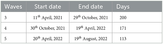
Table 1. Time and days for the waves used in the estimation of initial conditions.
To get the initial condition for asymptomatic individuals that was not given in the collected data, we used the study done by Kleynhans et al. [51]. Their studies reveal that the exact number of COVID-19 infections in Africa may be 97% higher than the number of confirmed reported cases. The rest of the initial conditions of state variables are taken from the data and are given below in Equation (33).
Initial conditions for susceptible and the asymptotic infectives are given by S0 = N − (E0 + Ia0 + Is + R0) and , respectively.
We considered the periodic transmission rate
is given as a piece-wise function below,
where
The parameter β is positive and denotes the maximum value of the transmission rate. Time-varying vaccination parameter m(t). We define our which falls between (0, 1], mx is the speed of the vaccination (called the vaccination efficacy) and tx is the start time of the implementation of the vaccine. For our numerical simulations, we fitted our model to the data starting from the third wave to the fifth wave, see Assan and Nyabadza [45] for first and second wave fitting. We added the damping to the fifth wave because that is when mandatory vaccination was implemented in South Africa. We used the function curve-fit from the python module scipy.optimize to fit our data which uses non-linear least squares to fit data to a functional form, see Figure 2.
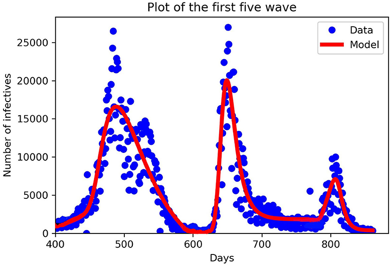
Figure 2. Fitting our mathematical model to the third, fourth, and fifth wave of data in piece-wise form. New cases in South Africa for the third, fourth, and fifth waves. The third wave from 11th April to 29th October 2021, the fourth wave from 30th October 2021 to 19th April, 2022 and the fifth wave from 20th April, 2022 to 19th August, 2022. The blue dots denote the new cases from the data, and the red lines denote our mathematical model prediction. We can see that in each wave our model constructed fitted well for the given parameters in Table 2.
In Table 2, we discuss in detail the values of the parameters used in Equation (11). When fitting Model (11) to the South African data obtained, we divided days according to the number of waves we have, starting with the third wave which occurred on the 400th day. When comparing the periodic transmission rate the fifth wave has a low transmission rate; this is due to the mandatory vaccination that was introduced by the government, which reduces the disease-induced death rate drastically. Parameter values used for plotting are within the range from the third to the fifth wave, see Figures 3–6.
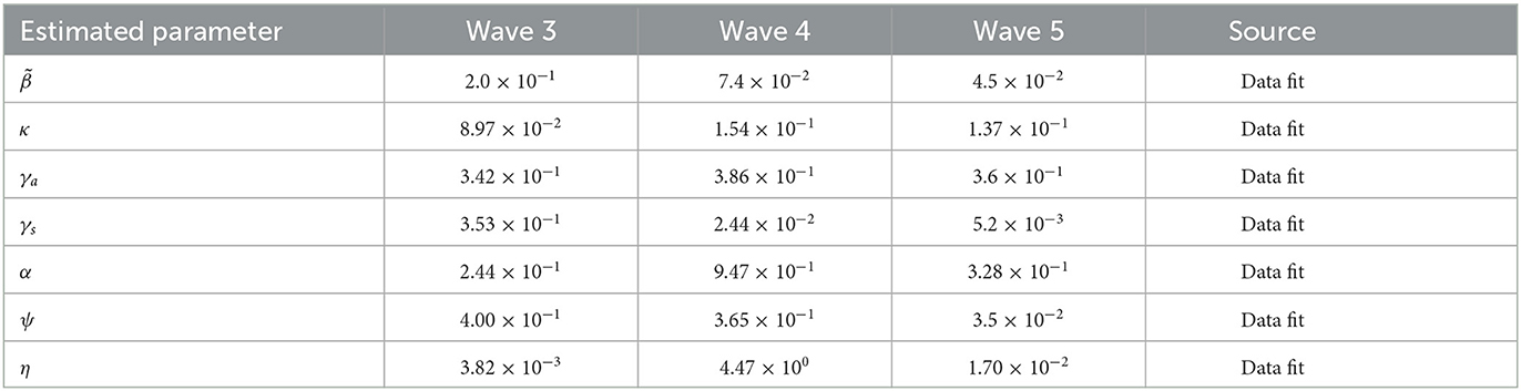
Table 2. Parameter estimation of the third, fourth, and fifth wave in South Africa in days.
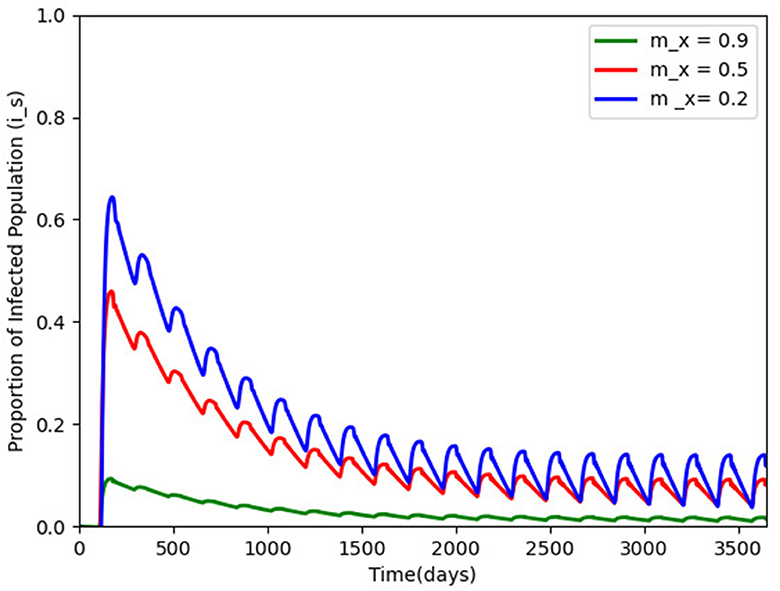
Figure 3. Proportion of infected humans for different vaccination efficacy; mx = 0.9, 0.5, and 0.2 and with other parameters made constant as in Table 2. The infection persists and a periodic solution with ω = 182.25 days forms after a long transient.
We hypothetically assume carry capacity K = 106, as a result of difficulties in estimating such a parameter, the removal rate of the virus is per day, and Lambda = 14, 000 and based on the model properties in Section 2.2, . We also chose and to be 10. Figure 3 gives the efficacy of the vaccination mx in the disease transmission. When mx is carried out to 0.9 (the green wave), the disease transmission reduces drastically, but the disease persists after a long transient with a periodic solution ω = 182 days.
Figure 4 gives the periodic threshold of R0 by varying the efficacy of the vaccination to see its effect on infection transmission. Figure 5 gives the maximum or minimum values of the vaccination speed (vaccination efficacy), which is (0, 1.5] and remains constant (disease dies out) from 1.5 and the upper bound does not make sense after mx = 1.5.
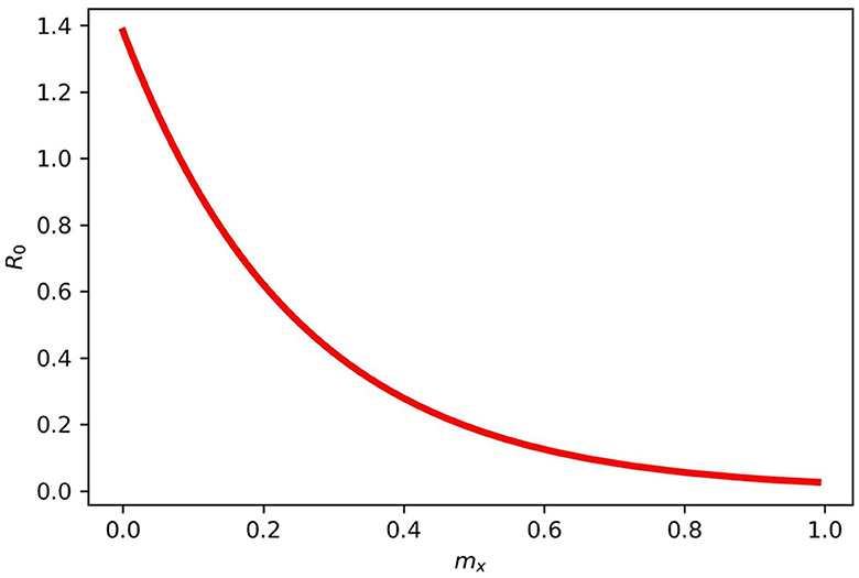
Figure 4. Gives the periodic threshold of R0 for various mx in model (2). When mx = 1, then R0 < 1, and if mx = 0, then R0 > 1.
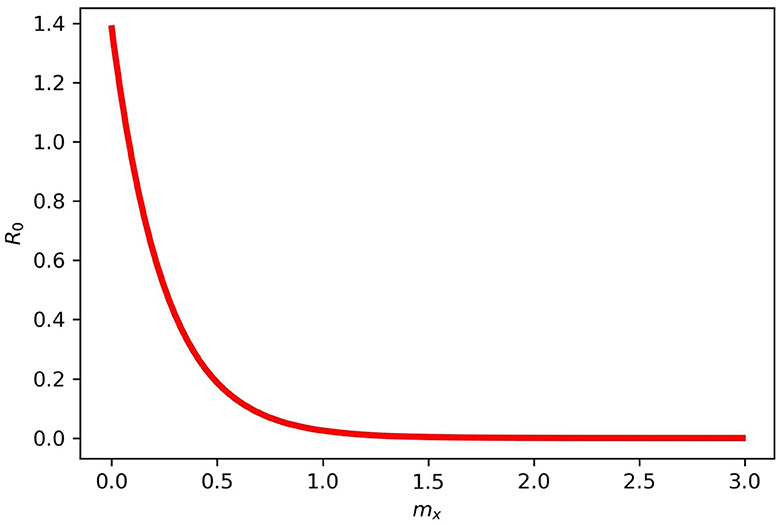
Figure 5. Maximum and minimum values for mx in model (2). mx = (0, 1.5] and does not make sense after 1.5 for the disease dies out completely.
Figure 6 gives two different initial conditions for the virus in the environment. The long-term behavior showed the same patterns, with infection moving toward a positive solution and a long oscillating transient, respectively, showing that a little shedding of the virus in the environment can sustain infection in the environment for the long term (see the Supplementary material for sample algorithm for some of the figures).

Figure 6. Pathogens density for different initial conditions (500 and 1, 000) over a period of 5 years of disease persistence and with the rest of the parameters being constant as defined in Table 2. The virus persists and a periodic solution with ω = 182.25 days forms after a long transient.
5. Conclusion and discussion
We presented a general non-autonomous COVID-19 model in a periodic environment. Seasonally variational factors have been incorporated into the incidence function δ and the pathogen function ζ. We proposed multiple periodic transmission pathways for COVID-19, human-to-human transmission, and human-to-environment transmission in this study. A detailed analysis of our model was conducted, and publicly reported data from the National Institute for Communicable Diseases was used for the study in South Africa.
Using the next infection operator, R0 = ρ(L), it was demonstrated that the disease-free equilibrium is globally asymptotically stable if R0 < 1. However, when R0 > 1, the disease persists uniformly, indicating that there is at least one positive periodic solution.
Our numerical simulation results demonstrate the application of our model to the COVID-19 outbreak in South Africa. Our mathematical model fits the reported data well, and through data fitting, we obtained some of our parameter values for other simulations. The South Africa data for COVID-19 show evidence of a seasonal pattern in the new cases, where peaks appear twice a year, that is in December to January and July to August due to various festive activities during these seasons. During the first four waves of COVID-19 in South Africa, non-pharmaceutical interventions were used as control measures. In this study, we proposed a control measure (vaccination), seasonality, and the role of the environment explaining the differences between the epidemic curves, starting from the third wave. A time-varying vaccination parameter m(t) was defined with the assumption that m(t) rises or falls exponentially. We implemented this in the fifth wave when the implementation of vaccination was mandatory in the South African population. We set m(t) to be between (0 − 1]; when m(t) = 1, then the epidemic spreads without any restrictions. However, m(t) can not be assumed to be one except when there are no control measures, and when m(t) = 0, then there is no epidemic. mx is the speed of the vaccination (vaccination efficacy).
We varied the efficacy of the vaccination on the infected population on a scale of 0.2, 0.5, and 0.9. This was done separately to see their effects on the disease transmission rate. It was observed that when vaccination has 0.5 efficacy, it slightly reduces the infection rate since half of the population will be aware of the government and policymakers' prevention strategies. When vaccination is carried out to 0.9 or a mandatory vaccination is carried out effectively, the transmission rate decreases substantially, reducing the infected population. In presenting the results of R0, we varied mx while keeping other parameters fixed, and our result indicates that when mx = 1, then R0 < 1, and when mx = 0, then R0 > 1. From our result, we found out that the parameter mx = (0, 1.5] remains constant after 1.5, that is, the disease dies out completely.
Our simulation results clearly show that individuals continue to shed the virus back into the environment as long as individuals are infected. Thus, an increased transmission rate causes more susceptible individuals to become infected. This study attempts to model COVID-19 by taking seasonality, control measures (vaccination), and the influence of the role of the environment. The findings have implications for developing initiatives and regulations aimed at reducing COVID-19 transmission in the presence of seasonality.
The model presented in the study is not without limitations. After vaccination, the periodic nature of the data somewhat vanished. The modeling of such a decline requires functions that reflect damped oscillations, which will be a valuable addition to the model. The model does not include aspects of hospitalization and intensive care, which were central to the pandemic. The inclusion of these would surely make the model more robust. The model does not capture heterogeneity observed in the disease, especially aspects of age, COVID-19 variants, long COVID-19, co-morbidities, and obesity. These were important determinants of disease progression and outcomes. Despite these limitations, the model presents some useful findings in the modeling of the different waves of COVID-19.
Data availability statement
The original contributions presented in the study are included in the article/supplementary material, further inquiries can be directed to the corresponding author.
Author contributions
All authors contributed to the formulation of the model, its review and analysis, and drafting and editing of the manuscript.
Funding
The Organization for Women in Science for the Developing World (OWSD) and Swedish International Development Cooperation Agency (SIDA) funded the study.
Acknowledgments
The authors are grateful to the Department of Mathematics and Applied Mathematics, University of Johannesburg for the production of this paper.
Conflict of interest
The authors declare that the research was conducted in the absence of any commercial or financial relationships that could be construed as a potential conflict of interest.
Publisher's note
All claims expressed in this article are solely those of the authors and do not necessarily represent those of their affiliated organizations, or those of the publisher, the editors and the reviewers. Any product that may be evaluated in this article, or claim that may be made by its manufacturer, is not guaranteed or endorsed by the publisher.
Supplementary material
The Supplementary Material for this article can be found online at: https://www.frontiersin.org/articles/10.3389/fams.2023.1142625/full#supplementary-material
References
1. Cao Y, Liu X, Xiong L, Cai K. Imaging and clinical features of patients with 2019 novel coronavirus SARS-CoV-2: a systematic review and meta-analysis. J Med Virol. (2020) 92:1449–59. doi: 10.1002/jmv.25822
2. Wang W, Zhao XQ. Threshold dynamics for compartmental epidemic models in periodic environments. J Dyn Differ Equat. (2008) 20:699–717. doi: 10.1007/s10884-008-9111-8
3. Gralinski LE, Menachery VD. Return of the Coronavirus: 2019-nCoV. Viruses. (2020) 12:135. doi: 10.3390/v12020135
4. CDCP. Centers for Disease Control and Prevention: 2019 novel coronavirus. (2019). Available online at: https://www.cdc.gov/coronavirus/2019-ncov (accessed October, 2022).
5. WHO. World Health Organization: coronavirus disease (COVID-19). (2019). Available online at: https://www.who.int/health-topics/coronavirus (accessed October, 2022).
6. Liu X, Zhang S. COVID-19: Face masks and human-to-human transmission. Influenza Other Respi Viru. (2020) 14:472. doi: 10.1111/irv.12740
7. WHO. Modes of transmission of virus causing COVID-19: implications for IPC precaution recommendations (2020). Available online at: https://www.who.int/news-room/commentaries/detail/modes-of-transmission-of-virus-causing-covid-19-implications-for-ipc-precaution-recommendations (accessed October, 2022).
8. Kampf G, Todt D, Pfaender S, Steinmann E. Persistence of coronaviruses on inanimate surfaces and their inactivation with biocidal agents. J Hospital Infect. (2020) 104:246–51. doi: 10.1016/j.jhin.2020.01.022
9. Yang C, Wang J. A mathematical model for the novel coronavirus epidemic in Wuhan, China. Mathemat Biosci Eng. (2020) 17:2708. doi: 10.3934/mbe.2020148
10. Sarkar K, Mondal J, Khajanchi S. How do the contaminated environment influence the transmission dynamics of COVID-19 pandemic? Eur Phys J Special Topics. (2022) 231:3697–716. doi: 10.1140/epjs/s11734-022-00648-w
11. Ellerin T. Coronavirus resource center (2020). Available online at: https://www.health.harvard.edu/diseases-and-conditions/coronavirus-resource-center (accessed October, 2022).
12. Stokel-Walker C. How long does SARS-CoV-2 stay in the body? BMJ. (2022) 377:e1555. doi: 10.1136/bmj.o1555
13. ECCMID. Longest known COVID-19 infection 505 days described by UK researchers. (2022). Available online at: https://www.eurekalert.org/news-releases/950412 (accessed December, 2022).
14. Pérez-Lago L, Aldámiz-Echevarría T, García-Martínez R, Pérez-Latorre L, Herranz M, Sola-Campoy PJ, et al. Different within-host viral evolution dynamics in severely immunosuppressed cases with persistent SARS-CoV-2. Biomedicines. (2021) 9:808. doi: 10.3390/biomedicines9070808
15. Li L, Li S, Pan Y, Qin L, Yang S, Tan D, et al. An immunocompetent patient with high neutralizing antibody titers who shed COVID-19 virus for 169 days China, 2020. China CDC Weekly. (2021) 3:688. doi: 10.46234/ccdcw2021.163
16. Rahmani A, Dini G, Leso V, Montecucco A, Vitturi BK, Iavicoli I, et al. Duration of SARS-CoV-2 shedding and infectivity in the working age population: a systematic review and meta-analysis. La Medicina del lavoro. (2022) 113:e2022014. doi: 10.23749/mdl.v113i2.12724
17. López L, Rodo X. A modified SEIR model to predict the COVID-19 outbreak in Spain and Italy: simulating control scenarios and multi-scale epidemics. Results Phys. (2021) 21:103746. doi: 10.1016/j.rinp.2020.103746
18. Liu X, Huang J, Li C, Zhao Y, Wang D, Huang Z, et al. The role of seasonality in the spread of COVID-19 pandemic. Environ Res. (2021) 195:110874. doi: 10.1016/j.envres.2021.110874
19. Wang H, Xu K, Li Z, Pang K, He H. Improved epidemic dynamics model and its prediction for COVID-19 in Italy. Appl Sci. (2020) 10:4930. doi: 10.3390/app10144930
20. Zhang R, Li Y, Zhang AL, Wang Y, Molina MJ. Identifying airborne transmission as the dominant route for the spread of COVID-19. Proc Nat Acad Sci. (2020) 117:14857–63. doi: 10.1073/pnas.2009637117
21. Nistal R, de la Sen M, Gabirondo J, Alonso-Quesada S, Garrido AJ, Garrido I. A study on COVID-19 incidence in Europe through two SEIR epidemic models which consider mixed contagions from asymptomatic and symptomatic individuals. Appl Sci. (2021) 11:6266. doi: 10.3390/app11146266
22. Khajanchi S, Sarkar K, Mondal J, Nisar KS, Abdelwahab SF. Mathematical modeling of the COVID-19 pandemic with intervention strategies. Results Phys. (2021) 25:104285. doi: 10.1016/j.rinp.2021.104285
23. Ojo MM, Peter OJ, Goufo EFD, Nisar KS. A mathematical model for the co-dynamics of COVID-19 and tuberculosis. Math Comput Simul. (2023) 207:499–520. doi: 10.1016/j.matcom.2023.01.014
24. Babasola O, Kayode O, Peter OJ, Onwuegbuche FC, Oguntolu FA. Time-delayed modelling of the COVID-19 dynamics with a convex incidence rate. Inform Med Unlocked. (2022) 35:101124. doi: 10.1016/j.imu.2022.101124
25. Rai RK, Khajanchi S, Tiwari PK, Venturino E, Misra AK. Impact of social media advertisements on the transmission dynamics of COVID-19 pandemic in India. J Appl Mathemat Comput. (2022) 68:19–44. doi: 10.1007/s12190-021-01507-y
26. Peter OJ, Panigoro HS, Abidemi A, Ojo MM, Oguntolu FA. Mathematical model of COVID-19 pandemic with double dose vaccination. Acta Biotheor. (2023) 71:9. doi: 10.1007/s10441-023-09460-y
27. Kammegne B, Oshinubi K, Babasola O, Peter OJ, Longe OB, Ogunrinde RB, et al. Mathematical modelling of the spatial distribution of a COVID-19 outbreak with vaccination using diffusion equation. Pathogens. (2023) 12:88. doi: 10.3390/pathogens12010088
28. Batabyal S. COVID-19: Perturbation dynamics resulting chaos to stable with seasonality transmission. Chaos, Solit Fractals. (2021) 145:110772. doi: 10.1016/j.chaos.2021.110772
29. Eccles R. An explanation for the seasonality of acute upper respiratory tract viral infections. Acta Otolaryngol. (2002) 122:183–91. doi: 10.1080/00016480252814207
30. Zoran MA, Savastru RS, Savastru DM, Tautan MN, Baschir LA, Tenciu DV. Exploring the linkage between seasonality of environmental factors and COVID-19 waves in Madrid, Spain. Process Safety Environ Protect. (2021) 152:583–600. doi: 10.1016/j.psep.2021.06.043
31. Matson MJ, Yinda CK, Seifert SN, Bushmaker T, Fischer RJ, van Doremalen N, et al. Effect of environmental conditions on SARS-CoV-2 stability in human nasal mucus and sputum. Emerg Infect Dis. (2020) 26:2276. doi: 10.3201/eid2609.202267
32. Yao M, Zhang L, Ma J, Zhou L. On airborne transmission and control of SARS-CoV-2. Sci Total Environ. (2020) 731:139178. doi: 10.1016/j.scitotenv.2020.139178
33. Chin AW, Chu JT, Perera MR, Hui KP, Yen HL, Chan MC, et al. Stability of SARS-CoV-2 in different environmental conditions. Lancet Microbe. (2020) 1:e10. doi: 10.1016/S2666-5247(20)30003-3
34. Huang Z, Huang J, Gu Q, Du P, Liang H, Dong Q. Optimal temperature zone for the dispersal of COVID-19. Sci Total Environ. (2020) 736:139487. doi: 10.1016/j.scitotenv.2020.139487
35. Van Doremalen N, Bushmaker T, Morris DH, Holbrook MG, Gamble A, Williamson BN, et al. Aerosol and surface stability of SARS-CoV-2 as compared with SARS-CoV-1. New England J Med. (2020) 382:1564–7. doi: 10.1056/NEJMc2004973
36. Ratnesar-Shumate S, Williams G, Green B, Krause M, Holland B, Wood S, et al. Simulated sunlight rapidly inactivates SARS-CoV-2 on surfaces. J Infect Dis. (2020) 222:214–22. doi: 10.1093/infdis/jiaa274
37. Chan JFW, Yuan S, Kok KH, To KKW, Chu H, Yang J, et al. A familial cluster of pneumonia associated with the 2019 novel coronavirus indicating person-to-person transmission: a study of a family cluster. Lancet. (2020) 395:514–23. doi: 10.1016/S0140-6736(20)30154-9
38. Daniel D. Mathematical model for the transmission of Covid-19 with nonlinear forces of infection and the need for prevention measure in Nigeria. J Infect Dis Epidemiol. (2020) 6:158. doi: 10.23937/2474-3658/1510158
39. NICD. The National Institute for Communicable Diseases: coronavirus pandemic. (2022). Available online at: https://www.nicd.ac.za (accessed January, 2023).
40. Suman R, Javaid M, Haleem A, Vaishya R, Bahl S, Nandan D. Sustainability of coronavirus on different surfaces. J Clin Exp Hepatol. (2020) 10:386–90. doi: 10.1016/j.jceh.2020.04.020
41. Hethcote HW, Levin SA. Periodicity in epidemiological models. In: Applied Mathematical Ecology. Berlin, Heidelberg: Springer Berlin Heidelberg (1989). p. 193–211. doi: 10.1007/978-3-642-61317-3_8
42. Wang J, Liao S. A generalized cholera model and epidemic-endemic analysis. J Biol Dyn. (2012) 6:568–89. doi: 10.1080/17513758.2012.658089
43. Zhang F, Zhao XQ. A periodic epidemic model in a patchy environment. J Math Anal Appl. (2007) 325:496–516. doi: 10.1016/j.jmaa.2006.01.085
44. Assan B, Nyabadza F, Landi P, Hui C. Modeling the transmission of Buruli ulcer in fluctuating environments. Int J Biomathem. (2017) 10:1750063. doi: 10.1142/S1793524517500632
45. Assan B, Nyabadza F. Mathematical modelling of COVID-19 with periodic transmission: The case of South Africa. Comput Mathem Method. (2022) 2022:9326843. doi: 10.1101/2022.06.22.22276298
46. Smith HL, Waltman P. The Theory of the Chemostat: Dynamics of Microbial Competition. vol 13 Cambridge: Cambridge University Press. (1995). doi: 10.1017/CBO9780511530043
47. Thieme HR. Convergence results and a Poincaré-Bendixson trichotomy for asymptotically autonomous differential equations. J Math Biol. (1992) 30:755–63. doi: 10.1007/BF00173267
48. Smith HL. Monotone Dynamical Systems: An Introduction to the Theory of Competitive and Cooperative Systems: An Introduction to the Theory of Competitive and Cooperative Systems. Providence, RI: American Mathematical Society. (2008). doi: 10.1090/surv/041
49. Zhao XQ. Dynamical Systems in Population Biology. vol 16 Cham: Springer. (2003). doi: 10.1007/978-0-387-21761-1
50. Worldometer. Countries in the world by population 2022. (2022). Available online at: https://www.worldometers.info/world-population/population-by-country/ (accessed May, 2022).
Keywords: vaccination, periodic transmission rate, basic reproduction number, stability analysis, parameter estimation
Citation: Assan B and Nyabadza F (2023) A COVID-19 epidemic model with periodicity in transmission and environmental dynamics. Front. Appl. Math. Stat. 9:1142625. doi: 10.3389/fams.2023.1142625
Received: 11 January 2023; Accepted: 27 September 2023;
Published: 24 October 2023.
Edited by:
Aurelio A. de los Reyes V, University of the Philippines Diliman, PhilippinesReviewed by:
Angelyn Lao, De La Salle University, PhilippinesOlumuyiwa James Peter, University of Medical Sciences, Ondo, Nigeria
Subhas Khajanchi, Presidency University, India
Copyright © 2023 Assan and Nyabadza. This is an open-access article distributed under the terms of the Creative Commons Attribution License (CC BY). The use, distribution or reproduction in other forums is permitted, provided the original author(s) and the copyright owner(s) are credited and that the original publication in this journal is cited, in accordance with accepted academic practice. No use, distribution or reproduction is permitted which does not comply with these terms.
*Correspondence: Farai Nyabadza, fnyabadza@uj.ac.za