Modeling and bifurcation analysis of tuberculosis with the multidrug-resistant compartment incorporating chemoprophylaxis treatment

Tuberculosis is a major health problem that contributes significantly to infectious disease mortality worldwide. A new challenge for society that demands extensive work toward implementing the right control strategies for Tuberculosis (TB) is the emergence of drug-resistant TB. In this study, we developed a mathematical model to investigate the effect of chemoprophylaxis treatment on the transmission of tuberculosis with the drug-resistant compartment. An analysis of stabilities is performed along with an investigation into the possibility of endemic and disease-free equilibrium. The qualitative outcome of the model analysis shows that Disease Free Equilibrium (DFE) is locally asymptotically stable for R₀ < 1, but the endemic equilibrium becomes globally asymptotically stable for R₀ > 1. A bifurcation analysis was performed using the center manifold theorem, and it was found that the model shows evidence of forward bifurcation. Furthermore, the sensitivity analysis of the model was thoroughly carried out, and numerical simulation was also performed. This study showed that administering chemoprophylaxis treatment to individuals with latent infections significantly reduces the progression of exposed individuals to the infectious and drug-resistant classes, ultimately leading to a reduction in the transmission of the disease at large.

1. Introduction

Tuberculosis is a major health problem that contributes significantly to infectious mortality worldwide, with approximately 10.4 million new case reports and 1.4 million mortality reports in 2015 [1]. It is a chronic disease that has existed for several millennia. This disease is caused by a type of bacteria known as Mycobacterium tuberculosis, and when a person with active pulmonary TB disease coughs or sneezes, they expel droplets containing TB bacteria which can be inhaled by a healthy individual, potentially causing them to contract the disease. Although TB cases are decreasing in many developed countries, they are growing in Asia, Africa, and eastern parts of Europe. A new challenge for society that demands extensive work toward implementing the right control strategies for TB is the emergence of drug-resistant TB. In 2015, an estimated 480,000 new cases of multidrug-resistant (MDR) TB were reported. These cases were resistant to isoniazid and rifampin, which are the two most successful anti-TB drugs [1]. This new wave of MDR-TB cases could potentially undermine existing TB control efforts due to increasing resistance to effective TB drugs [1]. Globally, 206,030 multidrug-resistant TB cases were identified and reported in 2019, representing a 10% growth from 186,883 in 2018 [2].

A mathematical model for controlling TB epidemiology was formulated by Ojo et al. [3] with the aim of examining the effect of vaccination on TB dynamics in a specified population. This study revealed that reducing contact with infected individuals and vaccinating susceptible groups with high efficacy vaccines can reduce the burden of the disease. According to Hethcote [4], the significance of mathematical models is worth mentioning in the planning, implementation, evaluation, and optimization of disease prevention, detection, control, and treatment-based programs. Different mathematical models are formulated and analyzed using a number of mathematical methods and tools, but the majority of the models constructed are of the susceptible-exposed-infected-recovered (SEIR) type. The first mathematical model that was used for the investigation of the transmission dynamics of TB was formulated by Waaler et al. [5]. The susceptible-infected-recovered (SIR) and SEIR transmission models of TB were proposed by Side et al. [6], and the Lyapunov method was implemented to indicate the disappearance of a disease if the basic reproduction number is ≤1 and vice versa.

A study by Bhunu et al. [7] presented the SEIR model of TB, incorporating treatment for infectious individuals and chemoprophylaxis for latently infected groups. It was also reported that the treatment of infectious individuals is more effective if implemented in the first years, as it clears active TB immediately. Hence, the contribution of chemoprophylaxis treatment is considered to be significant in controlling the progression of infectious TB to active TB. According to Young et al. [8], early diagnosis and adherence to a 6-month to 2-year treatment regimen can cure TB. An SIR model for TB was constructed by Fredlina et al. [9], and a fourth-order Runge–Kutta technique was used for numerical simulation. According to their results, the transmission of TB can be controlled by decreasing the transmission rate and increasing the recovery rate. As per the findings of Feng and Castillo-Chavez [10], researchers developed three different models of TB, and their detailed stability analysis was performed based on the reproduction number of the model. Furthermore, a non-linear deterministic model that incorporates treatment and case detection was suggested by Athithan and Ghosh [11]. In this study, the whole population was categorized into four compartments, such as susceptible, exposed, infected, and recovered classes, to investigate the transmission dynamics of TB.

Rafflesia [12] developed a TB model of the susceptible-exposed–infected (SEI) type, considering the vaccination effect. In this model, susceptible individuals are divided into the vaccinated and unvaccinated groups before administering the vaccine. Trauer et al. [13] proposed a model with the aim of exploring the transmission of tuberculosis in the Asia-Pacific region. A TB model formulated by Zhang et al. [14] shows a logical agreement with the real cases of TB in China. Desaleng and Koya [15] compartmentalized the individuals based on their level of exposure to the disease and developed a mathematical model to describe the population dynamics of the compartments. They obtained the disease-free equilibrium and epidemic equilibrium points as well as a formula for the reproduction number. They reported that TB propagation is high in densely populated areas and low in sparsely populated areas. Khan et al. [16] formulated a model of tuberculosis by dividing the latent class into fast and slow progressions.

Agusto [17] formulated a TB model incorporating treatment for infected individuals as well as chemoprophylaxis. Effective control programs for tuberculosis (TB) should include control mechanisms for chemoprophylaxis, disease relapse, and treatment. These strategies can reduce both the number of actively infected and latently infected individuals. The implementation of these control mechanisms is crucial for reducing the number of infected TB cases. One way of controlling the transmission rate of TB is by employing a preventative therapy, known as chemoprophylaxis, in latently infected individuals. If individuals with latent TB are given preventative therapy, it delays progression to the infectious stage, reducing transmission rates. This kind of treatment serves as a post-exposure prophylaxis vaccine. In this study, a mathematical model is developed by extending the model in the study of Ronoh et al. [18] with the assumption that some individuals move directly from the exposed group to the recovered group because of chemoprophylaxis treatment in addition to progression to the infected compartment. In the model constructed by Ronoh et al. [18], the transmission of TB with drug resistance effects is described by considering only one progression rate from the exposed group to the infected group without including chemoprophylaxis treatment for latent individuals. Thus, this study differs from the previous one in that this work incorporates chemoprophylaxis treatment for latent individuals. The majority of the features in the Ronoh et al. [18] study have been adopted into our model by making modifications.

2. Model description and formulation

Based on the status of the disease, we categorized the whole study population into five groups. These groups included susceptible individuals (S), individuals exposed to tuberculosis (E), infected individuals with active tuberculosis (I), individuals who develop drug-resistant TB (D), and recovered individuals (R). The total study population is, thus, given by N = S + E + I + D + R.

It is assumed that individuals are recruited into the susceptible group through natural births (B). Furthermore, the recruitment of individuals into the susceptible group is increased by individuals from the recovered group after losing their partial immunity at the rate (d) and is decreased by natural deaths at the rate (c) and exposure to TB at the rate (a). The force of infection (a) causes individuals in the susceptible group to move to the exposed group, resulting in an increase in the number of individuals in the exposed group. The population in the exposed group is further decreased by natural deaths at the rate (c), individuals moving to the recovered group at the rate (e) due to chemoprophylaxis treatment of latent individuals, and individuals flowing to the group of infected individuals at the rate (b) by developing active tuberculosis.

The size of the infected group is increased as individuals move from the exposed group and develop active tuberculosis at the rate (b). It is also reduced by natural deaths at the rate (c), disease-induced deaths at the rate (f), and the recovery of individuals due to prompt treatment at the rate (j). Additionally, the infected group is further reduced by the individuals developing drug resistance to the first-line treatment at the rate (g).

The drug-resistant group (D) is increased by the individuals from the infected group who become drug-resistant to the first-line treatment at the rate (g). It is also declined due to natural deaths at the rate (c), disease-induced deaths at the rate (h), and recovering individuals due to the second line of treatment at the rate (i).

One the one hand, the recovered group is increased by individuals who recover due to the second line of treatment at a rate (i), those who recover due to prompt treatment at the rate (j), and those individuals who recover due to chemoprophylaxis treatment of latent individuals at the rate (e). On the other hand, it is reduced by natural deaths at the rate (c) and those losing their partial immunity at the rate (d). The above description of the model is diagrammatically shown in Figure 1.

FIGURE 1

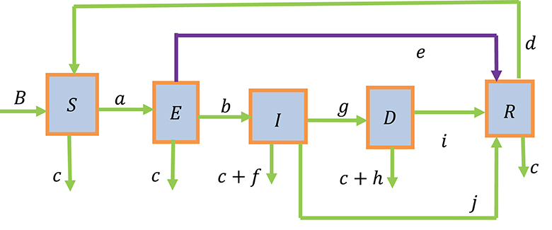
Figure 1. Flow diagram of the TB model.

The following system of five differential equations is obtained from the above flow diagram:

$\begin{array}{ll}\{\begin{array}{c}\frac{dS}{dt}=B-aSI-cS+dR\\ \frac{dE}{dt}=aSI-(c+b+e)E\\ \frac{dI}{dt}=bE-(c+f+j+g)I\\ \frac{dD}{dt}=gI-(c+h+i)D\\ \frac{dR}{dt}=jI-(c+d)R+iD+eE\end{array}& (1)\end{array}$

with the following initial condition S₀ > 0, E₀ ≥ 0, I₀ ≥ 0, D₀ ≥ 0, and R₀ ≥ 0.

3. Qualitative analysis

3.1. Existence of a solution and its uniqueness

Lemma 1: The solution of the model equation in Equation (1) together with the initial condition S(0) > 0, E(0) ≥ 0, I(0) ≥ 0, D(0) ≥ 0, R(0) ≥ 0 exist in $R_{+}^5$. That is, the solution of state variables S(t), E(t), I(t), D(t), and R(t) exist for all time t, and it remains in$R_{+}^5$.

Proof: The right hand side of Equation (1) can be expressed as follows:

$\begin{array}{l}\begin{array}{c}{f}_1(S,E,I,D,R)=B-aSI-cS+dR\\ f_2(S,E,I,D,R)=aSI-(c+b+e)E\\ f_3(S,E,I,D,R)=bE-(c+f+j+g)I\\ f_4(S,E,I,D,R)=gI-(c+h+i)D\\ f_5(S,E,I,D,R)=jI-(c+d)R+iD+eE.\end{array}\end{array}$

Let Ω denote the region given by $\text{Ω}=\left\{(S(t),E(t),I(t),D(t),R(t))\in R_{+}^5:N(t)\le \frac{B}{c}\right\}.$

Thus, by applying Theorem in Derrick and Grossman [19], Equation (1) has a unique solution if $\frac{\partial f_i}{\partial x_j},i,j=1,2,...,5$, are continuous and bounded in Ω. Using the notations x₁ = S, x₂ = E, x₃ = I, x₄ = D, x₅ = R, continuity and boundedness are verified as done below.

For f₁, we get $\left|\frac{\partial f_1}{\partial S}\right|=|-(aI+c)|<\infty ;\left|\frac{\partial f_1}{\partial E}\right|=0<\infty ;\left|\frac{\partial f_1}{\partial I}\right|=|-aS|<\infty ;\left|\frac{\partial f_1}{\partial D}\right|=0<\infty ;$ and $\left|\frac{\partial f_1}{\partial R}\right|=\left|d\right|<\infty$.

For f₂, we obtain $\left|\frac{\partial f_2}{\partial S}\right|=\left|aI\right|<\infty ;\left|\frac{\partial f_2}{\partial E}\right|=|-(c+b+e)|<\infty ;\left|\frac{\partial f_2}{\partial I}\right|=\left|aS\right|<\infty ;\left|\frac{\partial f_2}{\partial D}\right|=0<\infty ;$ and $\left|\frac{\partial f_2}{\partial R}\right|=0<\infty$.

For f₃, we find $\left|\frac{\partial f_3}{\partial S}\right|=0<\infty ;\left|\frac{\partial f_3}{\partial E}\right|=\left|b\right|<\infty ;\left|\frac{\partial f_3}{\partial I}\right|=|-(c+f+j+g)|<\infty ;\left|\frac{\partial f_3}{\partial D}\right|=0<\infty ;$ and $\left|\frac{\partial f_3}{\partial R}\right|=0<\infty$.

For f₄, we have $\left|\frac{\partial f_4}{\partial S}\right|=0<\infty ;\left|\frac{\partial f_4}{\partial E}\right|=0<\infty ;\left|\frac{\partial f_4}{\partial I}\right|=\left|g\right|<\infty ;\left|\frac{\partial f_4}{\partial D}\right|=|-(c+h+i)|<\infty ;\text{ and }\left|\frac{\partial f_4}{\partial R}\right|=0<\infty$.

Finally, for f₅ we obtain $\left|\frac{\partial f_5}{\partial S}\right|=0<\infty ;\left|\frac{\partial f_5}{\partial E}\right|=\left|e\right|<\infty ;\left|\frac{\partial f_5}{\partial I}\right|=\left|j\right|<\infty ;\left|\frac{\partial f_5}{\partial D}\right|=\left|i\right|<\infty ;$ and $\left|\frac{\partial f_5}{\partial R}\right|=|-(c+d)|<\infty$.

This shows that all the partial derivatives, $\frac{\partial f_i}{\partial x_j},i,j=1,2,...,5$, exist and they are continuous and bounded in Ω. Hence, by Lipchitz condition, the model (1) has a unique solution.

3.2. Positivity of the solutions

This section is aimed at finding non-negative solutions when dealing with human populations. It is crucial to verify whether all solutions of the system with a positive initial data remain positive for all time t ≥ 0. That is, the model Equation in (1) is epidemiologically meaningful and well-posed if all the state variables are shown to be non-negative for every t ≥ 0.

Theorem 2: If S(0), E(0), I(0), D(0), and R(0) are all non-negative, then the solutions S(t), E(t), I(t), D(t), and R(t) are all positive for t ≥ 0.

Proof: The positivity of S(t) can be verified by considering the first equation of the system of ordinary differential equation in Equation (1) as follows:

$\begin{array}{l}\frac{dS}{dt}=B-aSI-cS+dR.\end{array}$

While maintaining generality, the elimination of the positive terms in this equation results in an inequality $\frac{dS}{dt}\ge -aSI-cS=-(c+aI)S$. Thus, by using the separation of variable, the desired solution to this differential inequality can be obtained as follows:

$\begin{array}{l}\frac{dS}{S}\ge -(c+aI)dt\\ \Rightarrow {\displaystyle \int }\frac{dS}{S}\ge -{\displaystyle \int }(c+aI)dt\\ \Rightarrow lnS\ge -ct-a{\displaystyle \int }Idt+K,\text{ where }K\text{ is a constant }\\ \Rightarrow S\ge e^{-\left[ct+a\int Idt\right]+K}\\ \Rightarrow s\ge e^k{e}^{-\left[ct+a\int Idt\right]}\\ \Rightarrow s\ge P{e}^{-\left[ct+a\int Idt\right]},\text{ where }P=e^K\text{ is a constant}.\end{array}$

Using the initial condition S(0) = S₀, we get $S_0=P{e}^0=P.$

$\begin{array}{l}\Rightarrow s\ge S_0{e}^{-\left[ct+a\int Idt\right]}.\end{array}$

The function e^{−[ct+a ∫ Idt]} is a non-negative quantity since exponential functions are always non-negative regardless of the sign of the exponents. Therefore, S(t) ≥ 0.

Moreover, the positivity of E(t), I(t), D(t), and R(t) can be verified by taking the second, third, fourth, and fifth equations of the system of differential equations in Equation (1) and applying similar procedure.

This verifies that the state variables S(t), E(t), I(t), D(t), and R(t), which represent population size in the model, are positive quantities, and they remain in ${{ℝ}^5}_{+}$ for all time t.

3.3. Invariant region

Since the whole population at a given time t is expressed by N = S + E + I + D + R, differentiation of both sides with respect to t yields $\frac{dN}{dt}=\frac{d(S+E+I+D+R)}{dt}=\frac{dS}{dt}+\frac{dE}{dt}+\frac{dI}{dt}+\frac{dD}{dt}+\frac{dR}{dt}$. Hence, it follows that $\frac{dN}{dt}=B-c(S+E+I+D+R)-fI-hD=B-cN-fI-hD$.

Since f and h are non-negative, from $\frac{dN}{dt}=B-cN-fI-hD$, it can be obtained that

$\begin{array}{l}\frac{dN}{dt}\le B-cN.\\ \Rightarrow dN\le (0B-cN)dt.\\ \Rightarrow \frac{dN}{(B-cN)}\le dt.\\ \Rightarrow {\displaystyle \int }\frac{dN}{(B-cN)}\le {\displaystyle \int }dt.\\ \Rightarrow -\frac{1}{c}ln(B-cN)\le t+M,\text{ where }M\text{ is a constant}.\\ \Rightarrow ln(B-cN)\ge -(ct+cM).\\ \Rightarrow B-cN\ge e^{-(ct+cM)}.\\ \Rightarrow B-cN\ge e^{-ct}{e}^{-cM}.\\ \Rightarrow B-cN\ge K{e}^{-ct},\text{ where }K=e^{-cM}\text{ is a constant}.\end{array}$

Using the initial condition N(0) = N₀, we get $B-c{N}_0=K{e}^{-c(0)}.$

$\begin{array}{l}\Rightarrow B-c{N}_0=K.\end{array}$

Thus, it follows that $B-cN\ge (B-c{N}_0)e^{-ct}.\Rightarrow -cN\ge -B+(B-c{N}_0)e^{-ct}.$

$\begin{array}{l}\Rightarrow N\le \frac{B-(B-c{N}_0)e^{-ct}}{c}.\Rightarrow N\le \frac{B}{c}-\frac{(B-c{N}_0)e^{-ct}}{c}.\end{array}$

This shows that, as t → ∞, the population size $N\to \frac{B}{c},$implying that $0\le N\le \frac{B}{c}$. Thus, the feasibility region of the model becomes

$\begin{array}{l}\Omega =\left\{(S,E,I,D,R)\in {{ℝ}^5}_{+}:N\le \frac{B}{c}\right\}.\end{array}$

Thus, this model is mathematically well-posed and epidemiologically meaningful, and hence, it suffices to study the dynamics of this model in the region Ω.

3.4. Disease-free equilibrium and basic reproductive number

The computation of a steady-state solution corresponding to the model, termed as disease-free equilibrium point, is discussed in this section. It is a point where the disease vanishes from the population. That is, all the infected groups are zero, and the entire population will consist of only susceptible individuals. Thus, it can be found by setting the left hand side of Equation (1) equal to zero and letting E = 0, I = 0, D = 0, and R = 0.

$\begin{array}{ll}\{\begin{array}{c}B-aSI-cS+dR=0\\ aSI-(c+b+e)E=0\\ bE-(c+f+j+g)I=0\\ gI-(c+h+i)D=0\\ jI-(c+d)R+iD+eE=0\end{array}& (2)\end{array}$

Therefore, by solving these equations the disease free equilibrium point will be given by $(S_0,E_0,I_0,D_0,R_0)=\left(\frac{B}{c},0,0,0,0\right)$.

The reproductive number R₀ is explained as an average number of secondary cases that arise from an average primary case in a wholly susceptible population over the period of infection. It is used to predict whether the epidemic will spread or die out. According to Diekmann and Heesterbeek [20], the matrix of next generation of the proposed model is basically provided by FV⁻¹ and its reproductive number is $R_0=\rho (F{V}^{-1})$, where $F=\left[\frac{\partial F_i(x_0)}{\partial x_j}\right]$ and $V=\left[\frac{\partial V_i(x_0)}{\partial x_j}\right]$ and for i ≥ 1 compartments, there are 1 ≤ j ≤ m infected compartments only.

Rewriting the model equations in Equation (1) that correspond to the infected compartments yields

$\begin{array}{ll}\{\begin{array}{c}\frac{dE}{dt}=aSI-(c+b+e)E\\ \frac{dI}{dt}=bE-(c+f+j+g)I\\ \frac{dD}{dt}=gI-(c+h+i)D\end{array}& (3)\end{array}$

Then, the principle of next generation matrix is used to get f and v as follows

$\begin{array}{l}f=\left[\begin{array}{c}aSI\\ 0\\ 0\end{array}\right]=\left[\begin{array}{c}a\left(\frac{B}{c}\right)I\\ 0\\ 0\end{array}\right]=\left[\begin{array}{c}\frac{aB}{c}I\\ 0\\ 0\end{array}\right]\text{ and}\\ v=\left[\begin{array}{c}(c+b+e)E\\ (c+f+j+g)I-bE\\ (c+h+i)D-gI\end{array}\right].\end{array}$

Thus, the Jacobian matrix of f and v, by evaluating at disease free equilibrium (DFE), is given by F and V as follows:

$\begin{array}{l}F=\left[\begin{array}{ccc}0& \frac{aB}{c}& 0\\ 0& 0& 0\\ 0& 0& 0\end{array}\right]\text{ and }V=\left[\begin{array}{ccc}c+b+e& 0& 0\\ -b& c+f+j+g& 0\\ 0& -g& c+h+i\end{array}\right].\end{array}$

The inverse of V is, thus, obtained to be

$\begin{array}{l}{V}^{-1}=\left[\begin{array}{ccc}\frac{1}{c+b+e}& 0& 0\\ \frac{b}{(c+b+e)(c+f+j+g)}& \frac{1}{c+f+j+g}& 0\\ \frac{bg}{(c+b+e)(c+f+j+g)(c+h+i)}& \frac{g}{(c+f+j+g)(c+h+i)}& \frac{1}{(c+h+i)}\end{array}\right]\end{array}$

Next, the next generation matrix FV⁻¹ is computed and it becomes

$\begin{array}{r}F{V}^{-1}=\left[\begin{array}{ccc}0& \frac{aB}{c}& 0\\ 0& 0& 0\\ 0& 0& 0\end{array}\right]\left[\begin{array}{ccc}\frac{1}{c+b+e}& 0& 0\\ \frac{b}{(c+b+e)(c+f+j+g)}& \frac{1}{c+f+j+g}& 0\\ \frac{bg}{(c+b+e)(c+f+j+g)(c+h+i)}& \frac{g}{(c+f+j+g)(c+h+i)}& \frac{1}{c+h+i}\end{array}\right]\\ =\left[\begin{array}{ccc}\frac{abB}{c(c+b+e)(c+f+j+g)}& \frac{aB}{c(c+f+j+g)}& 0\\ 0& 0& 0\\ 0& 0& 0\end{array}\right].\end{array}$

Lastly, the eigenvalues for the next generation matrix FV⁻¹ are determined by solving the equation $|F{V}^{-1}-\text{λ}{I}_3|=0$. This implies that

$\begin{array}{l}|F{V}^{-1}-\lambda I_3|=\left|\begin{array}{ccc}\frac{abB}{c(c+b+e)(c+f+j+g)}-\lambda & \frac{aB}{c(c+f+j+g)}& 0\\ 0& 0-\lambda & 0\\ 0& 0& 0-\lambda \end{array}\right|=0\end{array}$

From this equation, one can obtain $\left(\frac{abB}{c(c+b+e)(c+f+j+g)}-\text{λ}\right)(0-\text{λ})(0-\text{λ})=0$. This shows that the eigenvalues are λ₁ = 0, λ₂ = 0, and ${\text{λ}}_3=\frac{abB}{c(c+b+e)(c+f+j+g)},$ where the dominant eigenvalue is ${\text{λ}}_3=\frac{abB}{c(c+b+e)(c+f+j+g)}$. Thus, the basic reproductive number, known as spectral radius of FV⁻¹, is given by

$\begin{array}{ll}{R}_0=\rho (F{V}^{-1})=\frac{abB}{c(c+b+e)(c+f+j+g)}.& (4)\end{array}$

Theorem 3: The DFE point $\left(\frac{B}{c},0,0,0,0\right)$ is locally asymptotically stable given that R₀ is smaller than one.

Proof: The proof of this Theorem follows directly from Theorem 2 in van den Driessche and Watmough [21].

Theorem 4: If R₀ < 1, the DFE point of the system in Equation (1) becomes globally asymptotically stable.

Proof: Let us think about the Lyapunov function defined on the positively invariant compact set Ω by

$\begin{array}{l}V=\frac{b}{(c+b+e)(c+f+j+g)}E+\frac{1}{(c+f+j+g)}I.\end{array}$

Here, V is non-negative and continuously differentiable on Ω. Thus, we obtain

$\begin{array}{l}\frac{dV}{dt}=\frac{b}{(c+b+e)(c+f+j+g)}\frac{dE}{dt}+\frac{1}{(c+f+j+g)}\frac{dI}{dt}\\ =\frac{b}{(c+b+e)(c+f+j+g)}\left[\frac{aB}{c}I-(c+b+e)E\right]\\ +\frac{1}{(c+f+j+g)}\left[bE-(c+f+j+g)I\right]\\ =\frac{abB}{c(c+b+e)(c+f+j+g)}I-\frac{b}{(c+f+j+g)}E\\ +\frac{1}{(c+f+j+g)}bE-I\\ =\frac{abB}{c(c+b+e)(c+f+j+g)}I-I\\ =\left(\frac{abB}{c(c+b+e)(c+f+j+g)}-1\right)I.\end{array}$

This implies that

$\begin{array}{l}\frac{dV}{dt}=(R_0-1)I.\end{array}$

To have $\frac{dV}{dt}\le 0$, we must have R₀ − 1 ≤ 0. Therefore, $\frac{dV}{dt}<0$ if R₀ < 1, and $\frac{dV}{dt}=0$ if and only if I = 0. Hence, a singleton set $E_0=\left(\frac{B}{c},0,0,0,0\right)$ is the biggest compact invariant set in Ω. Therefore, every solution of the model in Equation (1) with initial conditions in Ω approaches the disease-free equilibrium point as time t closes to infinity whenever R₀ < 1, according to LaSalle's invariant principle. This shows that the equilibrium point of a disease-free state is globally asymptotically stable if R₀ < 1 in Ω.

3.5. Endemic equilibrium and bifurcation analysis

The endemic equilibrium (EE) point, denoted by $E_{*}=(S^{*},E^{*},I^{*},D^{*},R^{*})$, is a steady-state solution which occurs whenever the disease persists in the population. To find the EE point, the model equations in Equation (1) are set equal to zero, and then, the resulting system is solved simultaneously to obtain

$\begin{array}{l}\{\begin{array}{l}{S}^{*}=\frac{B}{c{R}_0}\\ I^{*}=\frac{B\left(1-\frac{1}{R_0}\right)}{\frac{aB}{c{R}_0}-\frac{d}{(c+d)}\left[j+\frac{ig}{(c+h+i)}+\frac{e(c+f+j+g)}{b}\right]}\\ E^{*}=\frac{(c+f+j+g)}{b}{I}^{*}\\ D^{*}=\frac{g}{(c+h+i)}{I}^{*}\\ R^{*}=\frac{1}{(c+d)}\left[j+\frac{ig}{(c+h+i)}+\frac{e(c+f+j+g)}{b}\right]I^{*}.\end{array}\end{array}$

Since $a{S}^{*}-\frac{d}{(c+d)}\left[j+\frac{ig}{(c+h+i)}+\frac{e(c+f+j+g)}{b}\right]>0$, this endemic equilibrium will exist if B − cS^* > 0 is true.

$\begin{array}{r}\Rightarrow B-\frac{c(c+b+e)(c+f+j+g)}{ab}>0.\\ \Rightarrow B>\frac{c(c+b+e)(c+f+j+g)}{ab}.\\ \Rightarrow \frac{abB}{c(c+b+e)(c+f+j+g)}>1.\\ \Rightarrow R_0>1.\end{array}$

Thus, a system given in Equation (1) has a unique EE point whenever R₀ > 1.

3.5.1. Bifurcation analysis

The existence of an endemic equilibrium and its stability are determined by investigating the possibility of backward or forward bifurcation. To examine the possibility of a forward or backward bifurcation of model (2), we use the method introduced in Castillo-Chavez and Song [22]. This is performed by reassigning the following variables:

$\begin{array}{l}S=x_1,E=x_2,I=x_3,D=x_4,\text{and }R=x_5.\end{array}$

Thus, the system of Equation (1) can be expressed as

$\begin{array}{ll}\{\begin{array}{c}\frac{d{x}_1}{dt}=B-a{x}_1{x}_3-c{x}_1+d{x}_5\\ \frac{d{x}_2}{dt}=a{x}_1{x}_3-(c+b+e)x_2\\ \frac{d{x}_3}{dt}=b{x}_2-(c+f+j+g)x_3.\\ \frac{d{x}_4}{dt}=g{x}_3-(c+h+i)x_4\\ \frac{d{x}_5}{dt}=e{x}_2+j{x}_3+i{x}_4-(c+d)x_5\end{array}& (5)\end{array}$

Selecting a as the bifurcation parameter and then solving for a = a^* in (5), whenever R₀ = 1, gives

$\begin{array}{ll}{a}^{*}=\frac{c(c+b+e)(c+f+j+g)}{bB}.& (6)\end{array}$

The linearized matrix of system (6) about the disease-free equilibrium for a = a^* is

$\begin{array}{l}J\left(E^0,a^{{}^{*}}\right)\\ =\left[\begin{array}{ccccc}-c& 0& -\frac{a^{{}^{*}}B}{c}& 0& d\\ 0& -(c+b+e)& \frac{a^{{}^{*}}B}{c}& 0& 0\\ 0& b& -(c+f+j+g)& 0& 0\\ 0& 0& g& -(c+h+i)& 0\\ 0& e& j& i& -(c+d)\end{array}\right].& (7)\end{array}$

The Jacobian matrix in Athithan and Ghosh [11] possesses simple zero eigenvalues; thus, the center manifold theory is used to analyze the dynamics of the system (5) near a = a^*. Now, we get both the right and left eigenvectors for J(E⁰, a^*) corresponding to the zero eigenvalue. The eigenvector of the right side is given by $W={(w_1{w}_2{w}_3{w}_4{w}_5)}^T$ from Equation (7):

$\begin{array}{l}\left[\begin{array}{ccccc}-c& 0& -\frac{a^{*}B}{c}& 0& d\\ 0& -(c+b+e)& \frac{a^{*}B}{c}& 0& 0\\ 0& b& -(c+f+j+g)& 0& 0\\ 0& 0& g& -(c+h+i)& 0\\ 0& e& j& i& -(c+d)\end{array}\right]\left[\begin{array}{c}{w}_1\\ w_2\\ w_3\\ w_4\\ w_5\end{array}\right]\\ =\left[\begin{array}{c}0\\ 0\\ 0\\ 0\\ 0\end{array}\right].& (8)\end{array}$

Thus, the Equation (8) can be expressed as

$\begin{array}{ll}\{\begin{array}{c}-c{w}_1-\frac{a^{*}B}{c}{w}_3+d{w}_5=0\\ -(c+b+e)w_2+\frac{a^{*}B}{c}{w}_3=0\\ b{w}_2-(c+f+j+g)w_3=0\\ g{w}_3-(c+h+i)w_4=0\\ e{w}_2+j{w}_3+i{w}_4-(c+d)w_5=0.\end{array}& (9)\end{array}$

By computing the system in Equation (9), we obtain

$\begin{array}{l}{w}_1=\frac{d\left[(e(c+f+j+g)+bj)(c+h+i)+ibg\right]-(c+d)(c+b+e)(c+f+j+g)(c+h+i)}{c(c+d)(c+h+i)(c+f+j+g)}{w}_2,\end{array}$

$\begin{array}{l}{w}_2=w_2>0,\\ w_3=\frac{b}{(c+f+j+g)}{w}_2,\\ w_4=\frac{bg}{(c+f+j+g)(c+h+i)}{w}_2,\\ w_5=\frac{(e(c+f+j+g)+bj)(c+h+i)+ibg}{(c+d)(c+h+i)(c+f+j+g)}{w}_2.& (10)\end{array}$

Similarly, the eigenvector of the left side V = (v₁ v₂ v₃ v₄ v₅) in Equation (7) related to the zero eigenvalue is computed as

$\begin{array}{l}{\left[\begin{array}{c}{v}_1\\ v_2\\ v_3\\ v_4\\ v_5\end{array}\right]}^T\left[\begin{array}{ccccc}-c& 0& -\frac{a^{*}B}{c}& 0& d\\ 0& -(c+b+e)& \frac{a^{*}B}{c}& 0& 0\\ 0& b& -(c+f+j+g)& 0& 0\\ 0& 0& g& -(c+h+i)& 0\\ 0& e& j& i& -(c+d)\end{array}\right]\\ =\left[\begin{array}{c}0\\ 0\\ 0\\ 0\\ 0\end{array}\right].& (11)\end{array}$

Hence, the Equation (11) reduces to

$\begin{array}{ll}\{\begin{array}{c}-c{v}_1=0\\ -(c+b+e)v_2+b{v}_3+e{v}_5=0\\ -\frac{a^{*}B}{c}b{v}_1+\frac{a^{*}B}{c}{v}_2-(c+f+j+g)v_3+g{v}_4+j{v}_5=0.\\ -(c+h+i)v_4+i{v}_5=0\\ d{v}_1-(c+d)v_5=0\end{array}& (12)\end{array}$

By solving the system in Equation (10), we obtain

$\begin{array}{l}V=\left(0v_2\left(\frac{c+b+e}{b}\right)v_{2}00\right).\end{array}$

where v₂ > 0. Moreover, using the dot product rule W·V = 1, we can find out the expressions for v₂ and w₂ as

$\begin{array}{r}{w}_2=1,\\ v_2=\frac{1}{1+\frac{c+b+e}{c+f+j+g}}=\frac{c+f+j+g}{2c+f+j+g+b+e}.\end{array}$

Then, the local stability close to the bifurcation point a = a^* is verified by the signs of a′ and b′, which are defined using the center manifold theorem in Castillo-Chavez and Song [22] as follows:

$\begin{array}{r}{a}^{{}^{\prime }}={\displaystyle \sum _{k,i,j=1}^5}{v}_k{w}_i{w}_j\frac{{\partial }^2{f}_k}{\partial x_i\partial x_j}\left(E^0\right),\\ b^{{}^{\prime }}={\displaystyle \sum _{k,i=1}^5}{v}_k{w}_i\frac{{\partial }^2{f}_k}{\partial x_i\partial a}\left(E^0\right),& (13)\end{array}$

where

$\begin{array}{ll}\begin{array}{c}{f}_1=B-a{x}_1{x}_3-c{x}_1+d{x}_5\\ f_2=a{x}_1{x}_3-(c+b+e)x_2\\ f_3=b{x}_2-(c+f+j+g)x_3\\ f_4=g{x}_3-(c+h+i)x_4\\ f_5=e{x}_2+j{x}_3+i{x}_4-(c+d)x_5.\end{array}& (14)\end{array}$

We found a′ and b′ by examining only the non-zero components of the left eigenvectors v₂ and v₃ and taking into consideration the non-zero second-order partial derivatives of Equation (14), which yields

$\begin{array}{r}{a}^{{}^{\prime }}=-\frac{dcJH+b\left(c+f+g\right)\left(c+h\right)+bi\left(c+f\right)+cKJH}{c\left(c+d\right)HJ}\\ \left(\frac{ab}{J+K}\right)<0\text{ and}\\ b^{{}^{\prime }}=\frac{bB}{cJ}\left(\frac{1}{J+K}\right)>0,\end{array}$

where H = c + h + i, J = c + f + j + g, and K = c + b + e.

The coefficient b′ is positive, whereas the coefficient a′ is negative; thus, with the help of the center manifold theorem in equation Castillo-Chavez and Song [22], system in Equation (2) exhibits a forward bifurcation at R₀ = 1, and hence, the endemic equilibrium becomes locally asymptotically stable for R₀ > 1 but adequately near 1.

3.5.2. Stability of endemic equilibrium

Theorem 5: An endemic equilibrium E_* corresponding to system (1) becomes locally asymptotically stable whenever R₀ > 1 (but near to one).

Proof: This follows directly from the center manifold theorem, since a model that shows forward bifurcation has an endemic equilibrium that exhibits locally asymptotic stability if R₀ > 1 Akanni et al. [23].

Theorem 6: If R₀ > 1, the EE point of the system in Equation (1) becomes globally asymptotically stable.

Proof: Choose a Lyapunov function of the form

$\begin{array}{l}V=\frac{1}{2}(\left(S-S^{*}\right)+\left(E-E^{*}\right)+\left(I-I^{*}\right)\\ +\left(D-D^{*}\right)+{\left(R-R^{*}\right))}^2.\end{array}$

The derivative of V with regard to time (t) corresponding to system (1) is given by

$\begin{array}{l}\frac{dV}{dt}=(\left(S-S^{*}\right)+\left(E-E^{*}\right)+\left(I-I^{*}\right)\\ +\left(D-D^{*}\right)+\left(R-R^{*}\right))\frac{d}{dt}\left(S+E+I+D+R\right),\\ =(\left(S-S^{*}\right)+\left(E-E^{*}\right)+\left(I-I^{*}\right)\\ +\left(D-D^{*}\right)+\left(R-R^{*}\right))\frac{dN}{dt}.\end{array}$

Since $\frac{dN}{dt}\le B-cN$, we must have

$\begin{array}{r}\frac{dV}{dt}\le (\left(S-S^{*}\right)+\left(E-E^{*}\right)+\left(I-I^{*}\right)+\left(D-D^{*}\right)\\ +\left(R-R^{*}\right))\left(B-cN\right),\\ \le \left(N-\frac{B}{c}\right)\left(B-cN\right).\end{array}$

After rearrangement and simplification of the equation, we obtain

$\begin{array}{l}\frac{dV}{dt}\le -\frac{1}{c}{\left(B-cN\right)}^2.\end{array}$

Thus, $\frac{dV}{dt}\le 0$, and $\frac{dV}{dt}=0$ if and only if S = S^*, E = E^*, I = I^*, D = D^*, and R = R^*. Hence, a singleton set $E_{*}=\left(S^{*},E^{*},I^{*},D^{*},R^{*}\right)$ is the greatest positive invariant set in $\left\{(S^{*},E^{*},I^{*},D^{*},R^{*})\in \text{Ω}:\frac{dV}{dt}=0\right\}$. This indicates the global asymptotic stability of E_∗ for R₀ > 1 in Ω as a result of LaSalle's invariant principle.

4. Analysis of sensitivity of model parameters

Sensitivity analysis is usually carried out to establish the relative effect of model parameters on disease transmission.

Definition: The ratio of a relative difference in the variable to a relative difference in the parameter is termed as normalized forward sensitivity index of a variable to a parameter. When a variable is a differentiable function of the parameter, the sensitivity index may be alternatively defined via partial derivatives as $\frac{\partial R_0}{\partial n}\times \frac{n}{R_0}$.

The derivation of the sensitivity of R₀ to each of the parameters is, thus, carried out as follows:

$\begin{array}{r}\frac{\partial R_0}{\partial a}\times \frac{a}{R_0}=1>0,\\ \frac{\partial R_0}{\partial b}\times \frac{b}{R_0}=\frac{c+e}{c+b+e}>0,\\ \frac{\partial R_0}{\partial c}\times \frac{c}{R_0}=-\frac{c\left(2c+b+e+f+j+g\right)}{\left(c+b+e\right)\left(c+f+j+g\right)}<0,\\ \frac{\partial R_0}{\partial e}\times \frac{e}{R_0}=-\frac{e}{c+b+e}<0,\\ \frac{\partial R_0}{\partial f}\times \frac{f}{R_0}=-\frac{f}{c+f+j+g}<0,\\ \frac{\partial R_0}{\partial g}\times \frac{g}{R_0}=-\frac{g}{c+f+j+g}<0,\\ \frac{\partial R_0}{\partial j}\times \frac{j}{R_0}=-\frac{j}{c+f+j+g}<0.\end{array}$

From Table 1, it can easily be noticed that the force of infection parameter (a) and the progression rate to active tuberculosis parameter (b) have positive indices, showing that they are the most sensitive parameters toward the spread of this disease. This is because the basic reproductive number increases as their values are increased, implying that the average number of secondary case infection increases in the community. For instance, $\frac{\partial R_0}{\partial a}\times \frac{a}{R_0}=+1$means that, if the parameter a increases by 10%, then the reproduction number will increase by 10% and vice versa. Similarly, $\frac{\partial R_0}{\partial b}\times \frac{b}{R_0}=+0.77167$means that, if we increase the parameter b by 10%, the reproductive number R₀ will increase by 10 to 7.7167% and vice versa.

TABLE 1

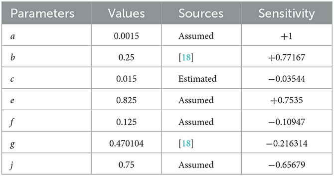
Table 1. Sensitivity index for R₀ with regard to the parameters in the model.

On the other hand, the parameters c, e, f, g, and j have negative indices which verify that they have an effect of minimizing the burden of the disease. For example, we can observe from $\frac{\partial R_0}{\partial e}\times \frac{e}{R_0}=-0.7535$ that a 10% increase (or decrease) in the parameter e leads to a 7.535% decrease (or increase) in the reproductive number R₀. Thus, it is very useful to note that enlargement of their values, while holding the other parameters constant, results in a decrease in the basic reproductive number. This shows that screening of latently infected individuals for chemoprophylaxis treatment reduces the progression rate to the infectious stage, and also, treatment of infectious people will stop them from transmitting the disease to healthy individuals, thereby leading to the reduction in disease transmission.

5. Numerical simulation, results, and discussion

Efforts were made to support the analytical results of the model by working with the numerical simulation of the model with the help of MATLAB ode45 solver. In addition to this, the effect of chemoprophylaxis treatment in the transmission dynamics of tuberculosis with the drug-resistant compartment is investigated.

For values of parameters a = 0.0015; b = 0.125; c = 0.015; d = 0.15; e = 0.725; f = 0.125; g = 0.470104; h = 0.575; i = 0.1106456; and j = 0.75, we computed the value R₀ = 0.7969 < 1. Hence, by using initial conditions S(0) = 5000, E(0) = 2500, I(0) = 500, D(0) = 75, R(0) = 400, and the above parameter values, we obtain the graph shown in Figure 2. From Figure 2, it can be seen that the susceptible and recovered groups go to their initial state values while the exposed, infected, and drug-resistant groups gradually approach zero with an increase in time. Therefore, it can be observed that the disease dies out in this case, which agrees with the analytical results of the model.

FIGURE 2

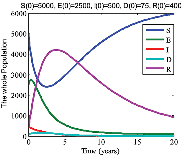
Figure 2. When R₀ = 0.7969 < 1.

By taking the values of parameters a = 0.0015; b = 0.45; c = 0.015; d = 0.15; e = 0.000725; f = 0.125; g = 0.1470104; h = 0.575; i = 0.11106456, and j = 0.25, we get R₀ = 13.4946 > 1. Now for initial conditions S(0) = 5000, E(0) = 2500, I(0) = 500, D(0) = 75, and R(0) = 400 and the above parameter values, we get the graph shown in Figure 3. From Figure 3, it can be noticed that the infected, drug-resistant, and recovered groups go to their initial state values while the susceptible and exposed groups decline with an increase in time. Thus, we see that the disease persists in this case and this also agrees with the analytical results of the model.

FIGURE 3

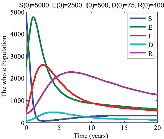
Figure 3. When R₀ = 13.4946 > 1.

5.1. Effect of chemoprophylaxis treatment on the exposed group

The preventive therapy (chemoprophylaxis treatment) using isoniazid decreases the risk of the initial episode of TB, which may occur in people who are exposed to the infection, have a latent infection, and have a recurrent episode of TB [24]. The mathematical model constructed by Ronoh et al. [18] did not consider the chemoprophylaxis treatment of latently infected individuals. Thus, this study has modified their model by incorporating the chemoprophylaxis treatment of latently infected individuals. To evaluate the effect of chemoprophylaxis treatment on the transmission dynamics of tuberculosis and compare the models, a simulation study of the new model was carried out with the chemoprophylaxis treatment parameter (e > 0) and without the chemoprophylaxis treatment parameter (e = 0). The numerical simulations were performed to view the effects on the exposed group, infected group, and drug-resistant group for three different values of the chemoprophylaxis treatment parameter e while keeping the other parameters constant as shown in Figures 4–6, respectively.

FIGURE 4

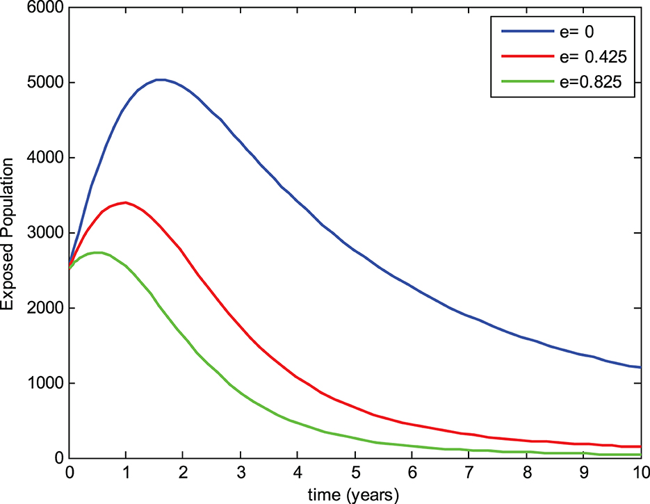
Figure 4. Effect of chemoprophylaxis treatment on the exposed group.

From Figure 4, it can be noticed that the number of individuals in the exposed group without chemoprophylaxis treatment is higher than the one with chemoprophylaxis treatment of exposed (latently infected) individuals. Additionally, the exposed group decreases whenever the chemoprophylaxis treatment parameter is increased. This shows that chemoprophylaxis treatment of latently infected individuals plays a significant role in reducing the transmission of tuberculosis.

5.2. Effect of chemoprophylaxis treatment on the infected group

In Figure 5, we can observe that the number of individuals in the infected group with the absence of chemoprophylaxis treatment is greater than the model with chemoprophylaxis treatment of latently infected individuals. Furthermore, the infected group also decreases as the chemoprophylaxis treatment parameter is increased. This implies that chemoprophylaxis treatment of latently infected individuals plays a great role in reducing the transmission of tuberculosis.

FIGURE 5

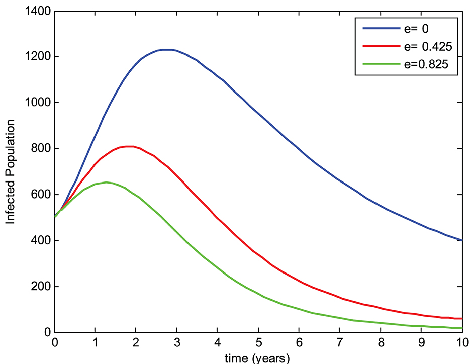
Figure 5. Effect of chemoprophylaxis treatment on the infected group.

5.3. Effect of chemoprophylaxis treatment on the drug-resistant group

Similarly, Figure 6 shows that the number of individuals in the drug-resistant group without chemoprophylaxis treatment is higher than in the model where chemoprophylaxis treatment is incorporated for latent individuals. Moreover, the drug-resistant group decreases as the chemoprophylaxis treatment parameter is increased, which proves that chemoprophylaxis treatment of latently infected individuals plays a great role in reducing the transmission of tuberculosis.

FIGURE 6

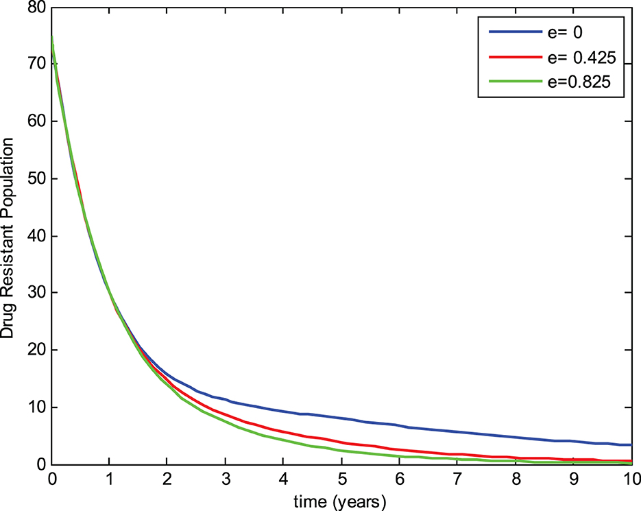
Figure 6. Effect of chemoprophylaxis treatment on the drug-resistant group.

In general, the numerical simulation obviously verifies that the model consisting of chemoprophylaxis treatment has a better result in reducing the transmission dynamics of TB with the drug-resistant compartment than the model without chemoprophylaxis treatment for latent individuals.

6. Conclusion

In this study, a mathematical model of tuberculosis with a drug-resistant compartment was formulated by considering chemoprophylaxis treatment for latently infected individuals. In the qualitative-based analysis of the model, a formula that described basic reproductive number R₀ was obtained by using the next generation matrix approach. The existence of the DFE point and the EE point was investigated, and their stabilities were also analyzed. The results of the analysis verified that the DFE point is locally asymptotically stable whenever R₀ < 1, and the EE point is globally asymptotically stable if R₀ > 1. Furthermore, bifurcation analysis was studied, sensitivity analysis of the model was carried out using the normalized forward sensitivity index, and numerical simulation of the model is also carried out using MATLAB ode45 software. It was checked that the result of the numerical simulation agrees with the analytical results of the model. Furthermore, from the results of sensitivity analysis and numerical simulation, it was found that treatment of latently infected individuals remarkably reduces the progression to the infected group. It also has an effect on reducing drug resistance development, which thereby leads to the reduction in disease transmission.

Data availability statement

The original contributions presented in the study are included in the article/supplementary material, further inquiries can be directed to the corresponding author.

Author contributions

DK: Conceptualization, Data curation, Formal analysis, Investigation, Methodology, Software, Validation, Visualization, Writing—original draft, Writing—review & editing. BB: Conceptualization, Formal analysis, Methodology, Supervision, Validation, Writing—review & editing. KR: Conceptualization, Formal analysis, Methodology, Supervision, Validation, Writing—review & editing, Investigation, Software, Visualization.

Funding

The author(s) declare that no financial support was received for the research, authorship, and/or publication of this article.

Conflict of interest

The authors declare that the research was conducted in the absence of any commercial or financial relationships that could be construed as a potential conflict of interest.

Publisher's note

All claims expressed in this article are solely those of the authors and do not necessarily represent those of their affiliated organizations, or those of the publisher, the editors and the reviewers. Any product that may be evaluated in this article, or claim that may be made by its manufacturer, is not guaranteed or endorsed by the publisher.

References

1. World Health Organization. Global Tuberculosis Report 2016. Geneva: WHO (2016).

Google Scholar

2. World Health Organization. Global Tuberculosis Report 2020. Geneva: WHO (2020).

Google Scholar

3. Ojo MM, Peter OJ, Goufo EFD, Panigoro HS, Oguntolu FA. Mathematical model for control of tuberculosis epidemiology. J Appl Mathematic Comput. (2023) 69:69–87. doi: 10.1007/s12190-022-01734-x

CrossRef Full Text | Google Scholar

4. Hethcote HW. The mathematics of infectious diseases. SIAM Rev. (2000) 42:599–653. doi: 10.1137/S0036144500371907

CrossRef Full Text | Google Scholar

5. Waaler H, Geser A, Andersen S. The use of mathematical models in the study of the epidemiology of tuberculosis. Am J Pub Health Nations Health. (1962) 52:1002–13. doi: 10.2105/AJPH.52.6.1002

CrossRef Full Text | Google Scholar

6. Side S, Sanusi W, Aidid MK, Sidjara S. Global stability of SIR and SEIR model for tuberculosis disease transmission with Lyapunov function method. Asian J Appl Sci. (2016) 9:87–96. doi: 10.3923/ajaps.2016.87.96

CrossRef Full Text | Google Scholar

7. Bhunu CP, Garira W, Mukandavire Z, Zimba M. Tuberculosis transmission model with chemoprophylaxis and treatment. Bull Math Biol. (2008) 70:1163–91. doi: 10.1007/s11538-008-9295-4

PubMed Abstract | CrossRef Full Text | Google Scholar

8. Young D, Stark J, Kirschner D. System biology of persistent infection: tuberculosis as a case study. Nat Rev Microbiol. (2008) 6:520–8. doi: 10.1038/nrmicro1919

PubMed Abstract | CrossRef Full Text | Google Scholar

9. Fredlina KQ, Oka TB, Dwipayana IM. SIR (suspectible, infectious, recovered) model for tuberculosis disease transmission. J Matematika. (2012) 1:52–8.

Google Scholar

10. Feng Z, Castillo-Chavez C. Mathematical Models for the Disease Dynamics of Tuberculosis. River Edge, NJ: World Scientific Publishing (1998).

Google Scholar

11. Athithan S, Ghosh M. Mathematical modelling of TB with the effects of case detection and treatment. Int J Dynam Control. (2013) 1:223–30. doi: 10.1007/s40435-013-0020-2

CrossRef Full Text | Google Scholar

12. Rafflesia U. Tuberculosis (TBC) transmission model, J. Gradien. (2014) 10:983–86.

Google Scholar

13. Trauer JM, Denholm JT, McBryde ES. Construction of a mathematical model for tuberculosis transmission in highly endemic regions of the Asia-pacific. J Theor Biol. (2014) 358:74–84. doi: 10.1016/j.jtbi.2014.05.023

PubMed Abstract | CrossRef Full Text | Google Scholar

14. Zhang J, Li Y, Zhang X. Mathematical modeling of tuberculosis data of china. J Theor Biol. (2015) 365:159–63. doi: 10.1016/j.jtbi.2014.10.019

PubMed Abstract | CrossRef Full Text | Google Scholar

15. Desaleng D, Koya PR. Modeling and analysis of malt-drug resistance tuberculosis in densly populated areas. Am J Appl Mathematics. (2016) 4:1–10. doi: 10.11648/j.ajam.20160401.11

CrossRef Full Text | Google Scholar

16. Khan MA, Ahmad M, Ullah S, Farooq M, Gul T. Modeling the transmission dynamics of tuberculosis in Khyber Pakhtunkhwa Pakistan. Math Comput Simul. (2019) 165:181–99. doi: 10.1016/j.matcom.2019.03.012

CrossRef Full Text | Google Scholar

17. Agusto FB. Optimal chemoprophylaxis and treatment control strategies of a tuberculosis transmission model. World J Model Simulat. (2009) 5:163–73.

Google Scholar

18. Ronoh M, Jaroudi R, Fotso P, Kamdoum V, Matendechere N, Wairimu J, et al. A mathematical model of tuberculosis with drug resistance effects. Applied Mathematics. (2016) 7:1303–16. doi: 10.4236/am.2016.712115

CrossRef Full Text | Google Scholar

19. Derrick NR, Grossman SL. Differential Equation With Application. Philippines: Addision Wesley Publishing Company, Inc. (1976).

Google Scholar

20. Diekmann O, Heesterbeek JA. Mathematical Epidemiology of Infectious Diseases: Model Building, Analysis and Interpretation. London: John Wiley and Sons (2000).

Google Scholar

21. van den Driessche P, Watmough J. Reproduction numbers and sub-threshold endemic equilibria for compartmental models of disease transmission. Math Biosci. (2002) 180:29–48. doi: 10.1016/S0025-5564(02)00108-6

PubMed Abstract | CrossRef Full Text | Google Scholar

22. Castillo-Chavez C, Song B. Dynamical models of tuberculosis and their applications. Math Biosci Eng. (2004) 1:361–404. doi: 10.3934/mbe.2004.1.361

PubMed Abstract | CrossRef Full Text | Google Scholar

23. Akanni JO, Olaniyi S, Akinpelu FO. Global asymptotic dynamics of a nonlinear illicit drug use system. J Appl Mathematic Comput. (2021) 66:39–60. doi: 10.1007/s12190-020-01423-7

CrossRef Full Text | Google Scholar

24. WHO. Implementing the WHO Stop TB Strategy: A Handbook for National Tuberculosis Control Programmes. Geneva: World Health Organization (2008).

Google Scholar