 Andrey A. Popov*Adrian Sandu
- Computational Science Laboratory, Department of Computer Science, Blacksburg, VA, United States
Data assimilation is a Bayesian inference process that obtains an enhanced understanding of a physical system of interest by fusing information from an inexact physics-based model, and from noisy sparse observations of reality. The multifidelity ensemble Kalman filter (MFEnKF) recently developed by the authors combines a full-order physical model and a hierarchy of reduced order surrogate models in order to increase the computational efficiency of data assimilation. The standard MFEnKF uses linear couplings between models, and is statistically optimal in case of Gaussian probability densities. This work extends the MFEnKF into to make use of a broader class of surrogate model such as those based on machine learning methods such as autoencoders non-linear couplings in between the model hierarchies. We identify the right-invertibility property for autoencoders as being a key predictor of success in the forecasting power of autoencoder-based reduced order models. We propose a methodology that allows us to construct reduced order surrogate models that are more accurate than the ones obtained via conventional linear methods. Numerical experiments with the canonical Lorenz'96 model illustrate that nonlinear surrogates perform better than linear projection-based ones in the context of multifidelity ensemble Kalman filtering. We additionality show a large-scale proof-of-concept result with the quasi-geostrophic equations, showing the competitiveness of the method with a traditional reduced order model-based MFEnKF.
1. Introduction
Data assimilation [1, 2] is a Bayesian inference process that fuses information obtained from an inexact physics-based model, and from noisy sparse observations of reality, in order to enhance our understanding of a physical process of interest. The reliance on physics-based models distinguishes data assimilation from traditional machine learning methodologies, which aim to learn the quantities of interest through purely data-based approaches. From the perspective of machine learning, data assimilation is a learning problem where the quantity of interest is constrained by prior physical assumptions, as captured by the model, and nudged toward the optimum solution by small amounts of data from imperfect observations. Therefore, data assimilation can be considered a form of physics-constrained machine learning [3, 4]. This work improves data assimilation methodologies by combining a mathematically rigorous data assimilation approach and a data rigorous machine learning algorithm through powerful techniques in multilevel inference [5, 6].
The ensemble Kalman filter [7–9] (EnKF) is a family of computational methods that tackle the data assimilation problem using Gaussian assumptions, and a Monte Carlo approach where the underlying probability densities are represented by ensemble of model state realizations. The ensemble size, i.e., the number of physics-based model runs, is typically the main factor that limits the efficiency of EnKF. For increasing the quality of the results when ensembles are small, heuristics correction methods such as covariance shrinkage [10–12] and localization [13–15] have been developed. As some form of heuristic correction is required for operation implementations of the ensemble Kalman filter, reducing the need for such heuristic corrections in operational implementations is an important and active area of research.
The dominant cost in operational implementations of EnKF is the large number of expensive high fidelity physics-based model runs, which we refer to as “full order models” (FOMs). A natural approach to increase efficiency is to endow the data assimilation algorithms with the ability to use inexpensive, but less accurate, model runs [16, 17], which we refer to as “reduced order models” (ROMs). ROMs are constructed to capture the most important aspects of the dynamics of the FOM, at a fraction of the computational cost; typically they use a much smaller number of variables than the corresponding FOM. The idea of leveraging model hierarchies in numerical algorithms for uncertainty quantification [18] and inference [19–22] is fast gaining traction in both the data assimilation and machine learning communities. Here we focus on two particular types of ROMs: a proper orthogonal decomposition (POD) based ROM, corresponding to a linear projection of the FOM dynamics onto a small linear subspace [23], and a ROM based on autoencoders [24], corresponding to a non-linear projection of the dynamics onto a small dimensional manifold.
The multifidelity ensemble Kalman filter (MFEnKF) developed by the authors [25, 26] combines the ensemble Kalman filter with the idea of surrogate modeling. The MFEnKF optimally combines the information obtained from both the full-order and reduced order surrogate model runs with information begotten from the observations. By posing the data assimilation problem in terms of a mathematically rigorous variance reduction technique—the linear control variate framework—MFEnKF is able to provide robust guarantees about the accuracy of the inference results.
While numerical weather prediction is the dominant driver of innovation in data assimilation literature [27], other applications can benefit from our multifidelity approach such as mechanical engineering [28–30] and air quality modeling [31–33].
The novel elements of this work are: (i) identifying a useful property of autoencoders, namely right invertibility, that aides in the construction of reduced order models, and (ii) deriving a theory for an extension to the MFEnKF through non-linear interpolation and projection techniques; we call the resulting approach nonlinear MFEnKF (NL-MFEnKF). The right-invertibility property ensures the consistency of the reduced state representation through successive applications of the projection and interpolation operators. Our proposed NL-MFEnKF technique shows an advantage on certain regimes of a difficult-to-reduce problem, the Lorenz'96 equations, and shows promise on a large-scale fluids problem, the quasi-geostrophic equations.
This paper is organized as follows. Section 2 discusses the data assimilation problem, provides background on control variates, the EnKF, and the MFEnKF, as well as ROMs and autoencoders. Section 3 introduces NL-MFEnKF, the non-linear extension to the MFEnKF. Section 4 presents the Lorenz'96 and quasi-geostrophic models and their corresponding POD-ROMs. Section 5 introduces the physics-informed autoencoder and practical methods of how to train them and pick optimal hyperparameters. Section 6 provides the results of numerical experiments. Concluding remarks are made in Section 7.
2. Background
Sequential data assimilation propagates imperfect knowledge about some physical quantity of interest through an imperfect model of a time-evolving physical system, typically with chaotic dynamics [34]. Without an additional influx of information about reality, our knowledge about the systems rapidly degrades, in the sense of representing the real system less and less accurately. Data assimilation uses noisy external information to enhance our knowledge about the system at hand.
Formally, consider a physical system of interest whose true state at time ti is XtiXti. The time evolution of the physical system is approximated by the dynamical model
where Xi is a random variable whose distribution describes our knowledge of the state of a physical process at time index i, and Ξi is a random variable describing the modeling error. In this paper we assume a perfect model (Ξi ≡ 0), as the discussion of model error in multifidelity methods is significantly outside the scope of this paper.
Additional independent information about the system is obtained through imperfect physical measurements of the observable aspects Yi of the truth Xti, i.e., through noisy observations
where the “observation operator” H maps the model space onto the observation space (i.e., selects the observable aspects of the state).
Our aim is to combine the two sources of information in a Bayesian framework:
where the density π(Xi) represents all our prior knowledge, π(Yi∣Xi) represents the likelihood of the observations given said knowledge, and π(Xi ∣ Yi) represents our posterior knowledge.
In the remainder of the paper we use the following notation. Let W and V be random variables. The exact mean of W is denoted by μW, and the exact covariance between W and V by ΣW,V. EW denotes an ensemble of samples of W, and ~μW and ~ΣW,V are the empirical ensemble mean of W and empirical ensemble covariance of W and V, respectively.
2.1. Linear Control Variates
Bayesian inference requires that all available information is used in order to obtain correct results [35]. Variance reduction techniques [36] are methods that provide estimates of some quantity of interest with lower variability. From a Bayesian perspective they represent a reintroduction of information that was previously ignored. The linear control variate (LCV) approach [37] is a variance reduction method that aims to incorporate the new information in an optimal linear sense.
LCV works with two vector spaces, a principal space 𝕏 and a control space 𝕌, and several random variables, as follows. The principal variate X is a 𝕏-valued random variable, and the control variate ^U is a highly correlated 𝕌-valued random variable. The ancillary variate U is a 𝕌-valued random variable, which is uncorrelated with the preceding two variables, but shares the same mean as ^U, meaning μU=μ^U. The linear control variate framework builds a new 𝕏-valued random variable Z, called the total variate:
where the linear “gain” operator S is used to minimize the variance in Z by utilizing the information about the distributions of the constituent variates X, ^U and U.
In this work 𝕏 and 𝕌 are finite dimensional vector spaces. The dimension of 𝕏 is taken to be n. The dimension of 𝕌 we denote by r when it is the reduced order model state space. When 𝕌 is the observation space, its dimension is denoted by m.
The following lemma is a slight generalization of [[37], Appendix].
LEMMA 1 (Optimal gain). The optimal gain S that minimizes the trace of the covariance of Z (4) is:
PROOF. Observe that,
meaning that the problem of finding the optimal gain is convex, and the minimum is unique and is defined by setting the first order optimality condition to zero,
to which the solution is given by (5) as required.
We first discuss the case where the principal and control variates are related by linear projection and interpolation operators,
where Θ is the projection operator, Φ is the interpolation operator, and ~X is the reconstruction of X.
We reproduce below the useful result [25, Theorem 3.1].
THEOREM 1. Under the assumptions that ^U and U have equal covariances, and that the principal variate residual is uncorrelated with the control variate, the optimal gain of (4) is half the interpolation operator:
Under the assumptions of Theorem 1 the control variate structure (4) is:
REMARK 1. Note that Theorem 1 does not require that any random variables are Gaussian. The above linear operator S remains optimal even for non-Gaussian random variables.
2.2. Linear Control Variates With Non-linear Transformations
While working with linear transformations is elegant, most practical applications require reducing the variance of a non-linear transformation of a random variable. We now generalize the control variate framework to address this case.
Following [36], assume that our transformed principal variate is of the form h(X), where h is some arbitrary smooth non-linear operator:
We also assume that the transformed control variate and the transformed ancillary variate are of the form g(^U) and g(U), respectively, where g is also some arbitrary smooth non-linear operator:
We define the total variate Zh in the space ℍ such that h(𝕏) ⊂ ℍ by:
with the optimal linear gain given by Lemma 1:
THEOREM 2. If ^U and U independently and identically distributed, and share the same mean and covariance, the control variate structure (13) holds, and the optimal linear gain is:
PROOF. As ^U and U are independently and identically distributed, they share the same mean and covariance under non-linear transformation,
In this case g(^U)-g(U) is unbiased (mean zero), and the control variate framework (14) can be applied. Thus, the optimal gain is given by (15) as required.
We now consider the case where the transformations of the principal variate and control variates represent approximately the same information,
and exist in the same space ℍ.
We now provide a slight generalization of Theorem 1 under non-linear transformation assumptions.
THEOREM 3. If the assumption of Theorem 2 hold, and the transformed principal variate residual is uncorrelated with the transformed control variate,
then the optimal gain is
where I is the identity operator.
PROOF. By simple manipulation of (15), we obtain:
2.3. The Ensemble Kalman Filter
The EnKF is a statistical approximation to the optimal control variate structure (4), where the underlying probability density functions are represented by empirical measures using ensembles, i.e., a finite number of realizations of the random variables. The linear control variate framework allows to combine multiple ensembles into one that better represents the desired quantity of interest.
Let EXbi∈ℝn×NX be an ensemble of NX realizations of the n-dimensional principal variate, which represents our prior uncertainty in the model state at time index i from (1). Likewise, let EHi(Xbi)=Hi(EXbi)∈ℝm×NX be an ensemble of NX realizations of the m-dimensional control observation state variate, which represents the same model realizations cast into observation space. Let EYi∈ℝm×NX be an ensemble of NX “perturbed observations,” which is a statistical correction required in the ensemble Kalman filter [9].
REMARK 2 (EnKF Perturbed Observations). Each ensemble member of the perturbed observations is sampled from a Gaussian distribution with mean the measured value, and the known observation covariance from (2):
The prior ensemble at time step i is obtained by propagating the posterior ensemble at time i − 1 through the model equations,
where the slight abuse of notation indicates an independent model propagation of each ensemble member. Application of the Kalman filter formula constructs an ensemble EXai describing the posterior uncertainty:
where the statistical Kalman gain is an ensemble-based approximation to the exact gain in Lemma 1:
REMARK 3 (Inflation). Inflation is a probabilistic correction necessary to account for the Kalman gain being correlated to the ensemble [38]. In inflation the ensemble anomalies (deviations from the statistical mean) are multiplied by a constant α > 1, thereby increasing the covariance of the distribution described by the ensemble:
2.4. The Multifidelity Ensemble Kalman Filter
In this section, we present the standard Multifidelity Ensemble Kalman Filter (MFEnKF) with linear assumptions on the model, projection, and observation operators, and Gaussian assumptions on all probability distributions.
The MFEnKF [25] merges the information from a hierarchy of models and the corresponding observations into a coherent representation of the uncertain model state. To propagate this representation forward in time during the forecast phase, it is necessary that the models are decoupled, but implicitly preserve some underlying structure of the error information. We make use of the linear control variate structure to combine this information in an optimal manner.
Without loss of generality we discuss here a bi-fidelity approach, where one full-order model is coupled to a lower-fidelity reduced-order model. A telescopic extension to multiple fidelities is provided at the end of the section. Instead of having access to one model M, assume that we have access to a hierarchy of models. In the bi-fidelity case, the principal space model (FOM) is denoted by MX and the control space model (ROM) is denoted by MU.
We now consider the total variate
that describes the prior total information from a model that evolves in principal space (Xbi) and a model that evolves in ancillary space (^Ubi and Ubi).
Assume that our prior total variate is represented by the three ensembles EXbi∈ℝn×NX consisting of NX realizations of the n-dimensional principal model state variate, E^Ubi∈ℝr×NX consisting of NX realizations of the r-dimensional control model state variate, and EUbi∈ℝr×NU consisting of NU realizations of the r-dimensional ancillary model state variate. Each of these ensembles has a corresponding ensemble of m-dimensional control observation space realizations.
MFEnKF performs sequential data assimilation using the above constituent ensembles, without having to explicitly calculate the ensemble of the total variates. The MFEnKF forecast step propagates the three ensembles form the previous step:
Two observation operators HXi and HUi cast the principal model and control model spaces, respectively, into the control observation space. In this paper we assume that he principal model space observation operator is the canonical observation operator (2):
and that the control model space observation operator is the canonical observation operator (2) applied to the linear interpolated reconstruction (42) of a variable in control model space:
Additionally, we define an (approximate) observation operator for the total model variate :
which, under the linearity assumptions on HXi of Theorem 3 and the underlying Gaussian assumptions on ^Ui and Ui of Theorem 2, begets that HZi=HXi. Even without the linearity assumption the definition (29) is operationally useful.
The MFEnKF analysis updates each constituent ensemble as follows:
with the heuristic correction to the means
applied in order to fulfill the unbiasedness requirement of the control variate structure:
The Kalman gain and the covariances are defined by the semi–linearization:
In order to ensure that the control variate ^U remains highly correlated to the principal variate X, at the end of each analysis step we replace the analysis control variate ensemble with the corresponding projection of the principal variate ensemble:
Some important properties of MFEnKF are:
• MFEnKF makes use of surrogate models to reduce the uncertainty in the full state.
• MFEnKF does not explicitly construct the total variates, and instead performs the assimilation on the constituent ensembles.
• Under Gaussian and linear assumptions, the sample mean of the MFEnKF is an unbiased estimate of the truth.
REMARK 4 (MFEnKF Perturbed observations). There is no unique way to perform perturbed observations (remark 2) in the MFEnKF. We will present one way in this paper. As Theorem 2 requires both the control and ancillary variates to share the same covariance, we utilize here the ‘control space uncertainty consistency’ approach. The perturbed observations ensembles in (30) is defined by:
where the scaling factor is s = 1. See [25, Section 4.2] for a more detailed discussion about perturbed observations.
REMARK 5 (MFEnKF Inflation). Similarly to the EnKF (see Remark 3), the MFEnKF also requires inflation in order to account for the statistical Kalman gain being correlated to its constituent ensembles. For a bi-fidelity MFEnKF, two inflation factors are required: αX which acts on the anomalies of the principal and control variates (as they must remain highly correlated) and αU which acts on the ensemble anomalies of the ancillary variate:
REMARK 6 (Deterministic EnKF flavors). Many deterministic flavors of the EnKF [2] are extendable to the MFEnKF. The DEnKF [39] in particular is trivially extendanble to the non-linear multifidelity approach identified in this work. It has been the authors' experience, however that the perturbed observation flavor of the EnKF is more robust in the multifidelity setting. The authors' suspect that this is the case precisely because of its stochastic nature, leading it to better account for model error-based inaccuracies in the surrogate models. Accounting for this type of model error is outside the scope of this work.
REMARK 7 (Cost of the MFEnKF). It is known from [25] that, given a full order model with cost CX with NX ensemble members and a reduced order model with cost CU and NU ensemble members, then the MFEnKF is more effective than a normal EnKF with N ensemble members whenever,
meaning that the optimal cost of the reduced order model is highly dependent on the desired full order ensemble size.
2.5. Autoencoders
We now generalize from the linear interpolation and projection assumed previously (8), and consider a class of non-linear projection and interpolation operators.
An autoencoder [24] is an artificial neural network consisting of two smooth components, an encoder θ and a decoder ϕ, such that given a variable X in the principal space, the variable
resides in the control space of the encoder. Conversely the reconstruction,
is an approximation to X in the principal space, and which in some optimal sense approximately recovers the information embedded in X. While the relative dimension n of the principal space is relatively high, the arbitrary structure of an artificial neural networks allows the autoencoder to learn the optimal r-dimensional (small) representation of the data.
2.6. Non-linear Projection-Based Reduced Order Models
The important information of many dynamical systems can be expressed with significantly fewer dimensions than the discretization dimension n [40]. For many infinite dimensional equations it is possible to construct a finite-dimensional inertial manifold that represents the dynamics of the system (including the global attractor). The Hausdorff dimension of the global attractor of some dynamical system is a useful lower bound for the minimal representation of the dynamics, though a representation of just the attractor is likely not sufficient to fully capture all the “useful” aspects of the data. For data-based reduced order models an important aspect is the intrinsic dimension [41] of the data. The authors are not aware of any formal statements relating the dimension of an inertial manifold and the intrinsic dimension of some finite discretization of the dynamics. We assume that reduced dimension r is sufficient to represent either the dynamics or the data, or both, and allows to build a “useful” surrogate model.
We will now discuss the construction of reduced order models for problems posed as ordinary differential equations. The following derivations are similar to those found in [42], but assume vector spaces and no re-centering.
Just like in the control variate framework in Section 2.1, the full order model resides in the principal space 𝕏 ⊂ ℝn and the reduced order model is defined in the space 𝕌 ⊂ ℝr, which is related to 𝕏 through the smooth non-linear projection (41).
Given an initial value problem in 𝕏:
and the projection operator (41), the induced reduced order model initial value problem in 𝕌 is defined by simple differentiation of U = θ(X), by dynamics in the space 𝕌,
As is common, the full order trajectory is not available during integration, as there is no bijection from 𝕏 to 𝕌, thus an approximation using the interpolation operator (42) that fully resides in 𝕌 is used instead:
Note that this is not the only way to obtain a reduced order model by using arbitrary projection and interpolation operators. It is however the simplest extension of the POD-based ROM framework.
REMARK 8 (Linear ROM). Common methods for finding projection and interpolation operators make a linear assumption (methods such as POD), thus, in the linear case (8) the reduced order model (45) takes the form
3. Non-linear Projection-Based MFEnKF
We extend MFEnKF to work with non-linear projection and interpolation operators. The new algorithm is named NL-MFEnKF. Since existing theoretical extensions of the linear control variate framework to the non-linear case [43] are not completely satisfactory, violating the assumption of an unbiased estimate of the total variate, we resort to several heuristic assumptions to construct this algorithm. Heuristic approaches that work well in practice are widely used in data assimilation literature [2].
The main idea is to replace the optimal control variate structure for linear projection and interpolation operators (10) with one that works with their non-linear counterparts (13):
We assume that ^U and U are independently and identically distributed, such that they obey the assumptions made in Theorem 2 and in Theorem 3 for the optimal gain.
Similar to MFEnKF (28), the control model space observation operator is the application of the canonical observation operator (2) to the reconstruction
with the other observation operators Equations (27, 29) defined as in the MFEnKF.
REMARK 9. It is of independent interest to explore control model space observation operators that are not of the form (48). For example, if the interpolation operator ϕ is created through an autoencoder, the control model space observation operator HU could similarly be a different decoder of the same latent space.
The MFEnKF equations (30) are replaced by their non-linear counterparts in a manner similar to what is done with non-linear observation operators,
where, as opposed to (30), there are now two Kalman gains, defined by:
Here we take a heuristic approach and use semi-linear approximations of the covariances, similar to (34) and (35). The perturbed observations are defined like in MFEnKF (Remark 4).
Figure 1 provides a visual diagram of both the forecast and analysis steps of the NL-MFEnKF algorithm.
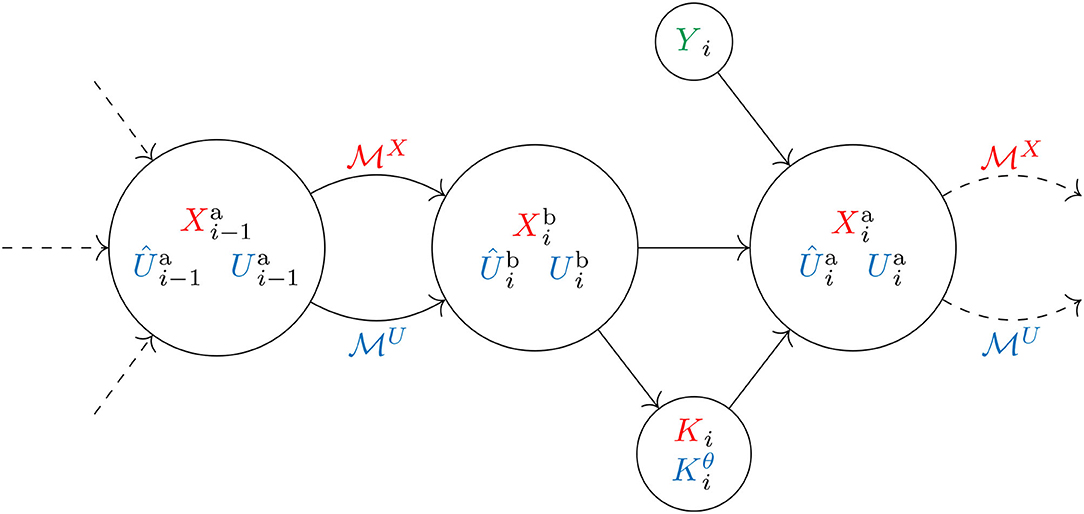
Figure 1. A visual diagram of the NL-MFEnKF algorithm. The random variables are represented by an ensemble of realizations, and the directional acyclic graph provides an explicit (infinite) causal graph.
REMARK 10 (Localization for the NL-MFEnKF). In operational data assimilation workflows, localization [2] is an important heuristic for the viability of the family of ensemble Kalman filter algorithms. While it is trivial to apply many B-localization techniques to the full-space Kalman gain (50), it is not readily apparent how one may attempt to do so for the reduced-space Kalman gain (51). Convolutional autoencoders [24] might provide an avenue for such a method, as they attempt to preserve some of the underlying spatial structure of the full space in the reduced space. An alternative is the use of R-localization, though, in the authors' view, there is a non-trivial amount of work to be done in order to formulate such a method.
3.1. NL-MFEnKF Heuristic Corrections
For linear operators the projection of the mean is the mean of the projection. This is however not true for general non-linear operators. Thus, in order to correct the means like in the MFEnKF (31), additional assumptions have to be made.
The empirical mean of the total analysis variate (47) [similar to (32)] is
We use it to find the optimal mean adjustments in reduced space. Specifically, we set the mean of the analysis principal variate to be the mean of the analysis total variate (52),
enforce the recorrelation of the principal and control variates (36) via
and define the control variate mean adjustment as a consequence of the above as,
Unlike the linear control variate framework of the MFEnKF (25), the non-linear framework of the NL-MFEnKF (47) does not induce a unique way to impose unbiasedness on the control-space variates. There are multiple possible non-linear formulations to the MFEnKF, and multiple possible heuristic corrections of the mean the ancillary variate. Here we discuss three approaches based on:
1. control space unbiased mean adjustment,
2. principal space unbiased mean adjustment, and
3. Kalman approximate mean adjustment,
each stemming from a different assumption on the relationship between the ancillary variate and the other variates.
3.1.1. Control Space Unbiased Mean Adjustment
The assumption that the control variate ^Uai and the ancillary variate Uai are unbiased in the control space implies that they share the same mean. The mean adjustment of ^Ua in (55) directly defines the mean adjustment of the ancillary variate:
The authors will choose this method of correction in the numerical experiments for both its properties and ease of implementation.
3.1.2. Principal Space Unbiased Mean Adjustment
If instead we assume that the control variate ϕ(^Ui) and the ancillary variate ϕ(Ui) are unbiased in the principal space (meaning that they have the same mean), then the mean of the total variate Zi (47) equals the mean of the principal variate Xi, a desirable property.
Finding a mean adjustment for Uai in the control space such that the unbiasedness is satisfied in the principal space is a non-trivial problem. Explicitly, we seek a vector ν such that:
resulting in the correction,
The solution to (57) requires the solution of an expensive nonlinear equation. Note that (57) is equivalent to (56) under the assumptions of Theorem 2, in the limit of large ensemble size.
3.1.3. Kalman Approximate Mean Adjustment
Instead of assuming that the control and ancillary variates are unbiased, we can consider directly the mean of the control-space total variate:
defined with the mean values in NL-MFEnKF formulas (49). The following adjustment to the mean of the ancillary variate:
is not unbiased with respect to the control variate in any space, but provides a heuristic approximation of the total variate mean in control space, and does not affect the principal variate mean.
3.2. Telescopic Extension
As in [[25], Section 4.5] one can telescopically extend the bi-fidelity NL-MFEnKF algorithm to a hierarchy of L+1 models of different fidelities. Assume that the nonlinear operator ϕℓ interpolates from the space of fidelity ℓ to the space of fidelity ℓ − 1, where ϕ1 interpolates to the principal space. A telescopic extension of (47) is
where the projection operator at each fidelity is defined as,
projecting from the space of fidelity ℓ to the principal space. The telescopic extension of the NL-MFEnKF is not analyzed further in this work.
4. Dynamical Models and the Corresponding POD-ROMs
For numerical experiments we use two dynamical systems: the Lorenz'96 model [44] and the Quasi-Geostrophic equations (QGE) [45–48].
For each of these models we construct two surrogates that approximate their dynamics. The first type of surrogate is a principal orthogonal decomposition-based quadratic reduced order model (POD-ROM), which is the classical approach to building the ROM. The second surrogate is an autoencoder neural network-based reduced order model (NN-ROM).
We will use the Lorenz'96 equations to test the methodology and derive useful intuition about the hyperparameters. For the POD-ROM and NN-ROMs for the Lorenz'96 equations we construct reduced order models (ROMs) for reduced dimension sizes of r = 7, 14, 21, 28, and 35.
We will use the Quasi-geostrophic equations to illustrate that our methodology can be applied in an operational setting. For both the POD-ROM and NN-ROMs we will build ROMs of a single reduced dimension size, r = 25.
The Lorenz'96, QGE, and corresponding the POD-ROM models are implemented in the ODE-test-problems suite [49, 50].
4.1. Lorenz'96
The Lorenz'96 model [44] can be conjured from the PDE [1, 51],
where the forcing parameter is set to F = 8. In the semi-discrete version y ∈ ℝn, and the nonlinear term is approximated by a numerically unstable finite difference approximation,
where ^I is a (linear) shift operator, and the linear operator ^D is a first order approximation to the first spatial derivative. The canonical n = 40 variable discretization with cyclic boundary conditions is used. The classical fourth order Runge-Kutta method is used to discretize the time dimension.
For the given discrete formulation of the Lorenz'96 system, 14 represents the number of non-negative Lyapunov exponents, 28 represents the rounded-up Kaplan-Yorke dimension of 27.1, and 35 represents an approximation of the intrinsic dimension of the system [calculated by the method provided by [52]]. To the authors' knowledge, the inertial manifold of the system, if it exists, is not known. The relatively high ratio between the intrinsic dimension of the system and the spatial dimension of the system makes constructing a reduced order model particularly challenging.
4.1.1. Data for Constructing Reduced-Order Models
The data to construct the reduced order models is taken to be 10, 000 state snapshots from a representative model run. The snapshots are spaced 36 time units apart, equivalent to 6 months in model time. The first 5, 000 snapshots provide the training data, and the next 5, 000 are taken as testing data in order to test the extrapolation power of the surrogate models.
4.1.2. Proper Orthogonal Decomposition ROM for Lorenz'96
Using the method of snapshots [53], we construct optimal linear operators, ΦT = Θ ∈ ℝr×n, such that the projection captures the dominant orthogonal modes of the system dynamics. The reduced order model approximation with linear projection and interpolation operators (46) is quadratic [similar to [54, 55]]
where the corresponding vector a, matrix B, and 3-tensor C are defined by:
4.2. Quasi-Geostrophic Equations
We will utilize the quasi-geostrophic equations (QGE) [45–48] as a proof-of-concept to showcase the proposed methodology in a more realistic setting. We follow the formulation used in [25, 55, 56],
where ω represents the vorticity, ψ is the corresponding streamfunction, Ro is the Rossby number, Re is the Reynolds number, and J represents the quadratic Jacobian term.
4.2.1. Data for Constructing Reduced-Order Models
For the QGE, we collect 10, 000 state snapshot points spaced 30 days apart, equivalent to about 0.327 time units in our discretization. As we wish to simulate a realistic online scenario, all data will be used for surrogate model training. The validation of the surrogates will be done through their practical use in the MFEnKF and NL-MFEnKF assimilation frameworks.
4.2.2. Proper Orthogonal Decomposition ROM for QGE
By again utilizing the method of snapshots on the vorticity, we obtain the optimal linear operators Φω∈ℝn×r Θω∈ℝr×n (orthogonal in some inner product space) that capture the dominant linear dynamics in the vorticity space. The linear operators corresponding to the streamfunction are then obtained by solving the Poisson equation
with Φψ being defined in a similar fashion, from which a quadratic ROM (65) is constructed as in [25]. In [25], it was shown that a reduced dimension of r = 25 is considered medium accuracy for the QGE, therefore this is the choice that we will use in numerical experiments.
5. Theory-Guided Autoencoder-Based ROMs
We now discuss building the neural network-based reduced order model (NN-ROM). Given the principal space variable X, consider an encoder θ that computes its projection U onto the control space (41), and a decoder ϕ that computes the reconstruction ~X (42).
Canonical autoencoders simply aim to minimize the reconstruction error:
which attempts to capture the dominant modes of the intrinsic manifold of the data. We identify a property of other reduced order modeling techniques which aims to preserve the physical consistency of the dynamics.
Recall the approximate dynamics in the reduced space (45) which provides an approximation to the reduced dynamics (44):
We derive a condition that creates a between the two tendencies in the right hand side of (70).
THEOREM 4. Assume the encoding of the reconstruction is the encoding of the full representation,
which we call the right-inverse property. Then the approximation (70) is bounded by,
PROOF. We have U = θ(X), ~X=ϕ(U)=ϕ(θ(X)). By the right-inverse-property (71),
Differentiating with respect to time,
and approximating with (45) similar to in (70),
then the term θ′(~X) now appears on both sides of the equation, and the error can be expressed as,
as required.
REMARK 11. The condition (72) is exact is difficult to enforce, as it would require the evaluation of the function f many times, which may be an intractable endeavor for large models. It is of independent interest to attempt and enforce this condition, or provide error bounds for certain flavors of models.
For POD (Section 4.1.2), the right-inverse property (71) is automatically preserved by construction and the linearity of the methods, as
by the orthogonality of Θ and Φ. Therefore,
For non-linear operators, the authors have not explicitly seen this property preserved, however, as the MFEnKF requires sequential applications of projections and interpolations, the authors believe that for the use-case outlined in this paper, the property is especially important.
It is of interest that the right invertibility property is implied by the mere fact that we are looking at preserving non-linear dynamics with the auto-encoder, but is otherwise agnostic to the type of physical system that we are attempting to reduce.
REMARK 12. Note that unlike the POD-ROM whose linear structure induces a purely r-dimensional initial value problem, the NN-ROM (45) still involves n-dimensional function evaluations. In a practical method it would be necessary to reduce the internal dimension of the ROM, however that is significantly outside the scope of this paper.
5.1. Theory-Guided Autoencoder-Based ROM for Lorenz'96
We seek to construct a neural network MNN that is a surrogate ROM for the FOM MX. We impose that the induced dynamics (45) makes accurate predictions, by not only capturing the intrinsic manifold of the data, but also attempting to capture the inertial manifold of the system. Explicitly, we wish to ensure that the surrogate approximation error in full space,
is minimized. We explicitly test the error in full space and not the reduced space, as the full space error is more relevant to the practitioner and for practical application of our methodology.
In this sense (45) would represent an approximation of the dynamics along a submanifold of the inertial manifold. In practice we compute (77) over a short trajectory in the full space started from a certain initial value, and a short trajectory in the latent space started form the projected initial value.
We will however not explicitly enforce (77) in the cost function, as that may be intractable for larger systems. We will instead only enforce the right-inverse property (71) by posing it as a weak constraint of the system.
Combining the canonical autoencoder reconstruction error term (69), and the right-inverse property (71), we arrive at the following loss function for each snapshot:
where the hyper-parameter λ represents the inverse relative weight of the mismatch of the right inverse property.
The full loss function, combining the cost functions for all T training snapshots:
can be minimized through typical stochastic optimization methods.
For testing we will look at two errors from the cost function, the reconstruction error,
which corresponds to the error in (69), and the right-invertibility error,
corresponds to the error in (71).
Aside from the two errors above, for testing, we additionally observe the propagation error,
which attempts to quantify the mismatch in (77) computed along K steps.
Similar to the POD model, we construct r-dimensional NN-based surrogate ROMs. To this end, we use one hidden layer networks with the element-wise tanh activation function for the encoder (41) and decoder (42):
where h is the hidden layer dimension, equal for both the encoder and decoder.
The corresponding linearization of the encoder is:
where (·)◦2 represents element-wise exponentiation, is required for the reduced order dynamics (45).
There are two hyper-parameters of interest, the hidden layer dimension, h, and the right-inverse weak-constraint parameter λ.
We consider the following hidden layer dimensions, h = 50, 100, 150, 200, 250, and 300. Additionally we consider the following values for right-inverse weak-constraint weights λ = 0, 1, 102, 104. We fix the propagation error parameter to K = 4, which corresponds to 24 h in model time, and observe all three errors (80), (81), and (82) on both the training and testing data sets.
We employ the ADAM [57] optimization procedure to train the NN and to produce the various ROMs. Gradients of the loss function are computed through automatic differentiation.
Figure 2 shows results from a representative set of models corresponding to different choices of the λ hyperparameter and the ROM dimension r = 28. As can be seen, the value of λ = 104 is too strict of a parameter, thus the cost function ignores all errors other than the right-invertibility constraint, while all other values of λ are produce viable models. The inclusion of the right-invertibility constraint not only improves the propagation error, but also makes the produced models less dependent on the hidden layer dimension h on the test data reconstruction.
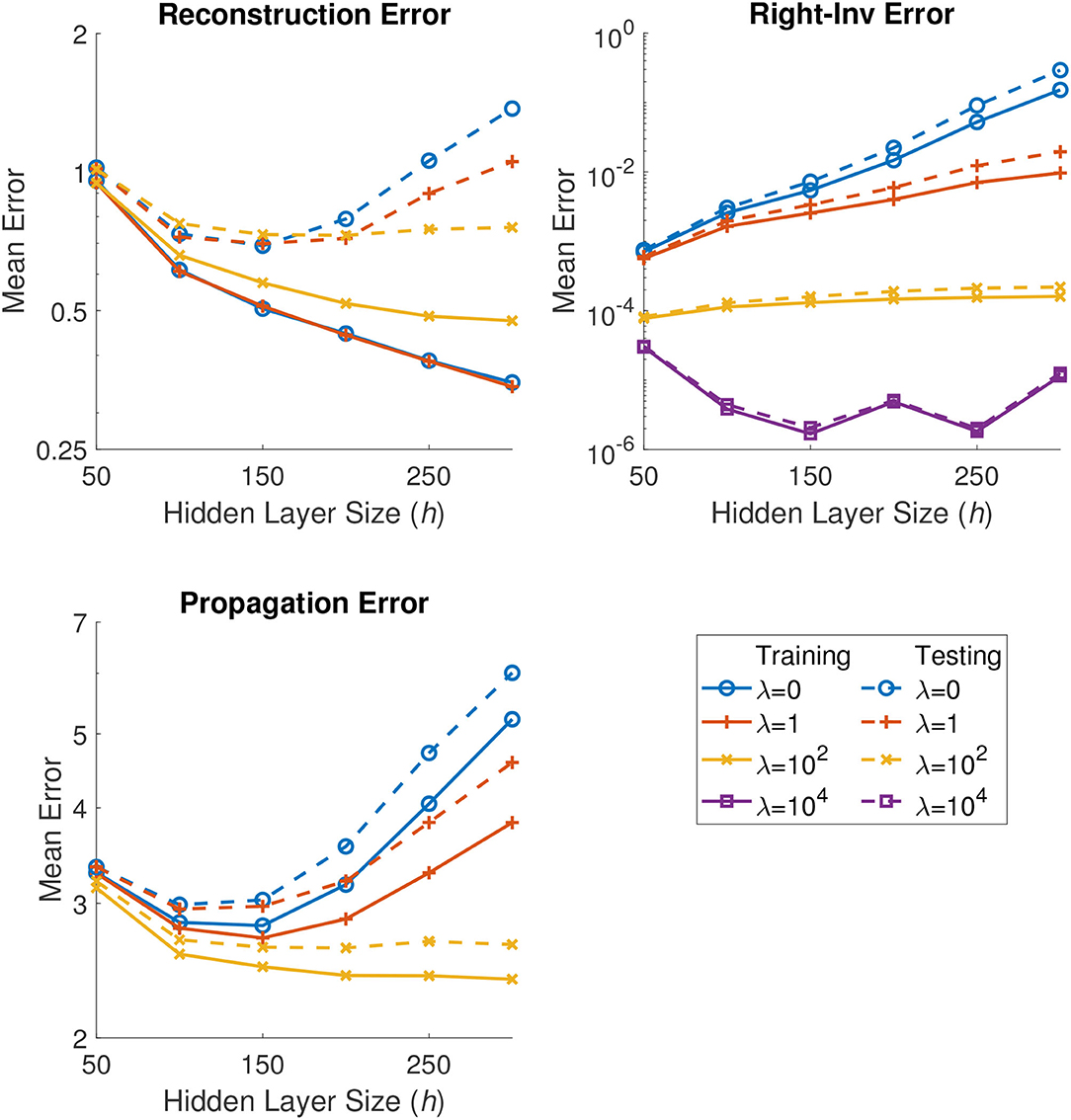
Figure 2. Results for an autoencoder-based ROM of dimension r = 28 approximating the Lorenz'96 FOM. The figure illustrates the mean error for the three error types that we observe: reconstruction error (80), the right invertibility error (81), and the propagation error (82), on both the training and testing data sets.
We consider the “best” model to be the one that which minimizes the propagation error (82) over the two parameters for each ROM dimension size. Table 1 shows the optimal parameter choices corresponding to each ROM dimension. The “best” models are chosen for the numerical experiments. Aside from the case r = 7, the optimal right-inverse constraint parameter is λ = 102.
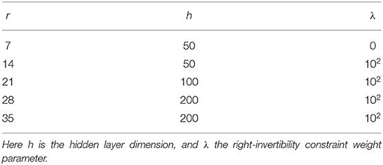
Table 1. A table of the optimal autoencoder parameters for the Lorenz '96 NN-ROM for different ROM dimensions r.
5.2. Theory-Guided Autoencoder-Based ROM for QGE
For a more realistic test case, we construct an autoencoder-based ROM for the QGE. The hyperparameters are chosen based on the information obtained using the Lorenz'96 model, rather than through exhaustive (and computationally-intensive) testing.
As in (83), we construct the encoder and decoder using
where σ is an approximation to the Gaussian error linear unit [58],
with all operations computed element-wise, and h is the hidden dimension size. The extra constant term C in (87) is a 2D-convolution corresponding to the stencil,
that aims to ensure that the resulting reconstruction does not have sharp discontinuities.
The choice of the activation function in (88) corresponds to a more realistic choice in state-of-the-art neural networks, and helps with choosing a smaller hidden dimension size.
Similar to Section 4.2.2, we make the choice that the reduced dimension size is r = 25. Informed by the Lorenz'96 NN-ROM, we take the hidden layer dimension h = 125, a medium value in between h = 100 and h = 150. We again use the hyperparameter value λ = 102.
6. Numerical Experiments
The numerical experiments with the Lorenz'96 model compare the following four methodologies:
1. Standard EnKF with the Lorenz'96 full order model;
2. MFEnKF with the POD surrogate model, an approach named MFEnKF(POD);
3. NL-MFEnKF with the autoencoder surrogate model, named NL-MFEnKF(NN); and
4. MFEnKF with the autoencoder surrogate model, named MFEnKF(NN).
Since MFEnKF does not support non-linear projections and interpolations, in MFEnKF(NN) the ensembles are interpolated into the principal space, and assimilated under the assumption that Θ = Φ = I.
For sequential data assimilation experiments we observe all 40 variables of the Lorenz'96 system, with an observation error covariance of Σηi, ηi = I. Observations are performed every 0.05 time units corresponding to 6 h in model time. We run 20 independent realizations (independent ensemble initializations) for 1, 100 time steps, but discard the first 100 steps for spinup.
The numerical experiments with the Quasi-geostrophic equations focus only on sequential data assimilation. We compare the following methodologies:
1. Standard EnKF with the QGE full order model;
2. MFEnKF with the POD surrogate model, an approach named MFEnKF(POD); and
3. NL-MFEnKF with the autoencoder surrogate model, named NL-MFEnKF(NN).
We observe 150 equally spaced variables directly, with an observation error covariance of Σηi, ηi = I. Observations are performed every 0.0109 time units corresponding to 1 day in model time. We run 5 independent realizations (independent ensemble initializations) for 350 time steps, but discard the first 50 steps for spinup.
In order to measure the accuracy of some quantity of interest with respect to the truth, we utilize the spatio-temporal root mean square error (RMSE):
throughout the rest of this section. Note here that the number of steps in a given experiment N is not necessarily the number of snapshot data point T.
6.1. Accuracy of ROM Models for Lorenz'96
Our first experiment is concerned with the preservation of energy by different ROMs, and seeks to compare the accuracy of NN-ROM against that of POD-ROM. For the Lorenz'96 model, we use the following equation [59] to model the spatio-temporal kinetic energy,
where T is the number of temporal snapshots of either the training or testing data. Table 2 shows the relative kinetic energies of the POD-ROM and the NN-ROM reconstructed solutions (42) (the energies of the reconstructed ROM solutions are divided by the kinetic energy of the full order solution) for both the training and testing data.
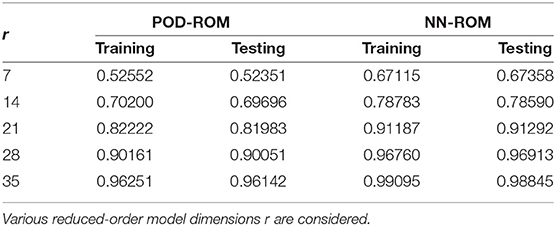
Table 2. Relative kinetic energies preserved by the reconstructions of the POD-ROM and the NN-ROM solutions of the Lorenz'96 system on both the training and testing data.
The results lead to several observations. First, the NN-ROM always preserves more energy than the POD-ROM. We have achieved our goal to build an NN-ROM that is more accurate than the POD-ROM. Second, the NN-ROMs with dimensions r = 21 and r = 28 preserve as much energy as the POD-ROMs with dimension r = 28 and r = 35, respectively. Intuitively this tells us that they should be just as accurate. Third, all the models preserve almost as much energy on the training as on the testing data, meaning that the models are representative over all possible trajectories.
6.2. Impact of ROM Dimension for Lorenz'96
The second set of experiments seeks to learn how the ROM dimension affects the analysis accuracy for the various multifidelity data assimilation algorithms.
We take the principal ensemble size to be NX = 32, and the surrogate ensemble sizes equal to NU = r − 3, in order to always work in the undersampled regime. All multifidelity algorithms (Sections 3, 2.4) are run with inflation factors αX = 1.05 and αU = 1.01. The traditional EnKF using the full order model is run with an ensemble size of N = NX and an inflation factor α = 1.06 to ensure stability. The inflation factors were chosen by careful hand-tuning to give a fair shot to all algorithms and models.
The results are shown in Figure 3. For the “interesting” dimensions r = 28, and r = 35, the NL-MFEnKF(NN) performs significantly better than the MFEnKF(POD). For a severely underrepresented ROM dimension of r = 7, r = 14, and r = 21 the MFEnKF(POD) outperforms the NL-MFEnKF(NN). The authors believe that this is due to the fact that a non-linear ROM size of less that r = 28 dimensions (the rounded-up Kaplan-Yorke dimension) is not sufficient to represent the full order dynamics without looking at additional constraints.
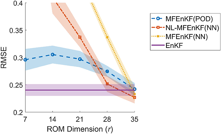
Figure 3. Lorenz'96 analysis RMSE vs. ROM dimension (r) for three multifidelity data assimilation algorithms and the classical EnKF. Ensemble sizes are NX = 32 and NU = r − 3. Error bars show two standard deviations. The inflation factor for the surrogate ROMs is fixed at αU = 1.01, the inflation of α = 1.07 is used for the EnKF, and αX = 1.05 is used for all other algorithms.
Of note is that, excluding the case of r = 35, the MFEnKF(NN) based on the standard MFEnKF method in the principal space is the least accurate among all algorithms, indicating that the non-linear method presented in this paper is truly needed for models involving non-linear model reduction.
We note that for r = 35, the suspected intrinsic dimension of the data, the NL-MFEnKF(NN) outperforms the EnKF, both in terms of RMSE and variability within runs. This is additionally strengthened by the results of the MFEnKF(NN) assimilated in the principal space, as it implies that there is little-to-no loss of information in the projection into the control space.
We believe that these are very promising results, as they imply that simply capturing the Kaplan-Yorke dimension and properly accounting for the non-linearity of the system could potentially bring in surrogates defined by non-linear operators to data assimilation research.
6.3. Ensemble Size and Inflation for Lorenz'96
Our second to last set of experiments focuses on the particular ROM dimension r = 28, as we believe that it is representative of an operationally viable dimension reduction, covering the dimensionality of the global attractor, and experimentally it is the sweet spot where the NL-MFEnKF(NN) beats all others except EnKF.
For each of the four algorithms we vary the principal ensemble size NX = N, and the principal inflation factor αX = α. As before, we set the control ensemble size to NU = r − 3 = 25 and the control-space inflation factor to αU = 1.01.
Figure 4 shows the spatio-temporal RMSE for various choices of ensemble sizes and inflation factors. The results show compelling evidence that NL-MFEnKF(NN) is competitive when compared to MFEnKF(POD); the two methods have similar stability properties for a wide range of principal ensemble size NX and principal inflation αX, but NL-MFEnKF(NN) yields smaller analysis errors for almost all scenarios for which the two methods are stable.
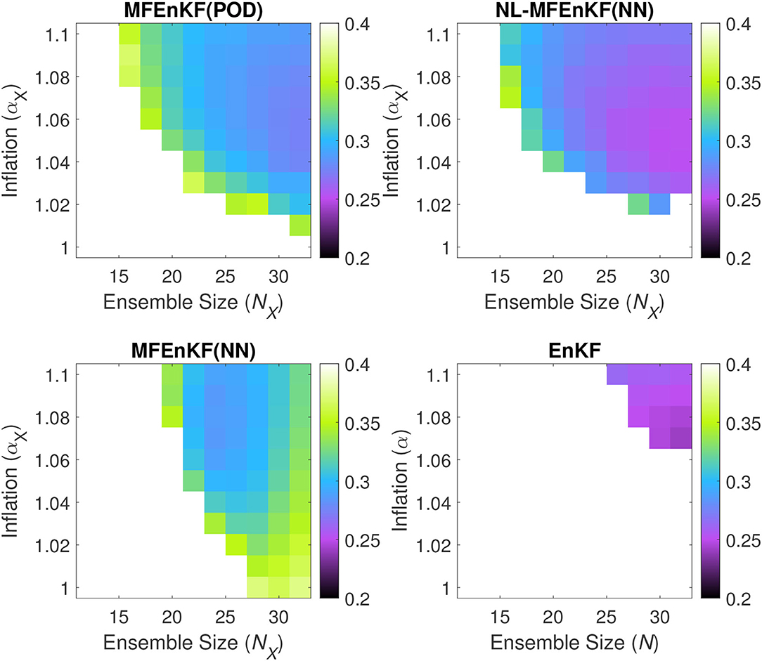
Figure 4. Lorenz'96 analysis RMSE for four data assimilation algorithms and various values of the principal ensemble size NX and inflation factor αX. The surrogate ROM size is fixed to r = 28 with ensemble size of NU = 25 and inflation of αU = 1.01. The (top left) represents the MFEnKF with a POD-ROM surrogate, the (top right) represents the NL-MFEnKF with a NN-ROM, the (bottom left) represents the MFEnKF with a NN-ROM surrogate assimilated in the principal space, and the (bottom right) represents the classical EnKF.
For a few points with low values of principal inflation αX, the NL-MFEnKF(NN) is not as stable as the MFEnKF(POD). This could be due to either an instability in the NN-ROM itself, in the NL-MFEnKF itself, or in the projection and interpolation operators.
An interesting observation is that the MFEnKF(NN), which is assimilated naively in the principal space, becomes less stable for larger ensemble sizes NX. One possible explanation for this is that the ensemble mean estimates become more accurate, thus the bias between the ancillary and control variates is amplified in (4), and more error is introduced from the surrogate model. This is in contrast to most other ensemble based methods, including all others in this paper, whose error is lowered by increasing ensemble size.
6.4. Ensemble Size and Inflation for QGE
Our last set of experiments focuses on the quasi-geostrophic equations. We use the POD-ROM developed in Section 4.2.2, and the NN-ROM discussed in Section 5.2.
As before, for each of the three algorithms we vary the principal ensemble size NX = N and principal inflation αX = α. In order to better visualize the results, we fix the control ensemble size to NU = 12, and the control inflation factor to αU = 1.05.
Figure 5 shows the spatio-temporal RMSE for various choices of ensemble sizes and inflation factors. The results provide evidence for the validity of the NL-MFEnKF approach for large-scale data assimilation problems.
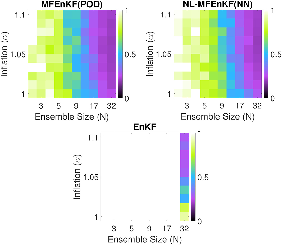
Figure 5. QGE analysis RMSE for four data assimilation algorithms and various values of the principal ensemble size NX and inflation factor αX. The surrogate ROM size is fixed to r = 25 with ensemble size of NU = 12 and inflation of αU = 1.05. The (top left) represents the MFEnKF with a POD-ROM surrogate, the (top right) represents the NL-MFEnKF with a NN-ROM, and the (bottom) represents the classical EnKF.
For similar values of inflation and ensemble size, the MFEnKF with a POD surrogate is comparable to the NL-MFEnKF with an autoencoder-based surrogate. Both multilevel filters significantly outperform the standard EnKF. The authors believe that these results show convincingly that the NL-MFEnKF formulation is valid for surrogates based on non-linear projection and interpolation.
7. Conclusions
The multifidelity ensemble Kalman filter (MFEnKF) uses a linear control variate framework to increase the computational efficiency of data assimilation; the state of the FOM is the principal variate, and a hierarchy of linear projection ROMs provide the control variates. In this work, the linear control variate framework is generalized to incorporate control variates built using non-linear projection and interpolation operators implemented using autoencoders. The approach, named NL-MFEnKF, enables the use of a much more general class of surrogate models than MFEnKF.
We identify the right-invertibility property of autoencoders as an important feature to support the construction of non-linear reduced order models. This property has previously not been preserved by autoencoders. We propose a methodology for building ROMs based on autoencoders that weakly preserves this property, and show that enforcing this property enhances the prediction accuracy over the standard approach.
We use these elements to construct NL-MFEnKF that extends the multifidelity ensemble Kalman filter framework to work with nonlinear surrogate models. The results obtained in this paper indicate that reduced order models based on non-linear projections that fully capture the intrinsic dimension of the data provide excellent surrogates for use in multifidelity sequential data assimilation. Moreover, nonlinear generalizations of the control variate framework result in small approximation errors, and thus the assimilation can be carried out efficiently in the space of a nonlinear reduced model.
Our Numerical experiments with both small scale (Lorenz '96) and medium scale (QGE) models show that the non-linear multifidelity approach has clear advantages over the linear multifilidety approach when the reduced order models are defined by non-linear couplings, and over the standard EnKF for similar high-fidelity ensemble sizes.
From the point of view of machine learning, the major limitations are the constructions of projection and interpolation operators, that do not account for the spatial features of the models, and the model propagation, which does not attempt to utilize state-of-the-art methods such as recurrent neural network models.
From the point of view of data assimilation, there are three limiting factors for the applicability of our method to operational workflows. The first is the use of the perturbed observations ensemble Kalman filter, the second is the absence of localization in our framework, and the third is the absence of model error both for the full-order and surrogate models.
One potential avenue of future research would be into adaptive inflation techniques for multifidelity data assimilation algorithms similar in vein to [60].
Future work addressing all the problems and research avenues above would lead to the successful application of the NL-MFENKF to operational problems such as numerical weather prediction.
Data Availability Statement
The raw data supporting the conclusions of this article will be made available by the authors, without undue reservation.
Author Contributions
AP performed the numerical experiments and wrote the first draft. All authors contributed to the concept and design of the study. All authors contributed to manuscript revision, read, and approved the submitted version.
Funding
This work was supported by DOE through award ASCR DE-SC0021313, by NSF through award CDS&E–MSS 1953113.
Conflict of Interest
The authors declare that the research was conducted in the absence of any commercial or financial relationships that could be construed as a potential conflict of interest.
Publisher's Note
All claims expressed in this article are solely those of the authors and do not necessarily represent those of their affiliated organizations, or those of the publisher, the editors and the reviewers. Any product that may be evaluated in this article, or claim that may be made by its manufacturer, is not guaranteed or endorsed by the publisher.
Acknowledgments
The authors would like to thank the rest of the members from the Computational Science Laboratory at Virginia Tech, and Traian Iliescu from the Mathematics Department at Virginia Tech.
References
1. Reich S, Cotter C. Probabilistic Forecasting and Bayesian Data Assimilation. Cambridge: Cambridge University Press (2015). doi: 10.1017/CBO9781107706804
2. Asch M, Bocquet M, Nodet M. Data assimilation: methods, algorithms, and applications. SIAM. (2016) 29:2318–31. doi: 10.1137/1.9781611974546
3. Karpatne A, Atluri G, Faghmous JH, Steinbach M, Banerjee A, Ganguly A, et al. Theory-guided data science: a new paradigm for scientific discovery from data. IEEE Trans Knowl Data Eng. (2017) 29:2318–31. doi: 10.1109/TKDE.2017.2720168
4. Willard J, Jia X, Xu S, Steinbach M, Kumar V. Integrating physics-based modeling with machine learning: a survey. arXiv preprint arXiv:200304919. (2020). doi: 10.48550/arXiv.2003.04919
5. Giles MB. Multilevel Monte Carlo path simulation. Oper Res. (2008) 56:607–17. doi: 10.1287/opre.1070.0496
6. Giles MB. Multilevel Monte Carlo methods. Acta Numer. (2015) 24:259–328. doi: 10.1017/S096249291500001X
7. Evensen G. Sequential data assimilation with a nonlinear quasi-geostrophic model using Monte Carlo methods to forecast error statistics. J Geophys Res. (1994) 99:10143–62. doi: 10.1029/94JC00572
8. Evensen G. Data Assimilation: the Ensemble Kalman Filter. Heidelberg: Springer Science & Business Media (2009).
9. Burgers G, van Leeuwen PJ, Evensen G. Analysis scheme in the ensemble Kalman Filter. Month Weath Rev. (1998) 126:1719–24. doi: 10.1175/1520-0493(1998)126<1719:ASITEK>2.0.CO;2
10. Nino-Ruiz ED, Sandu A. Efficient parallel implementation of DDDAS inference using an ensemble Kalman filter with shrinkage covariance matrix estimation. Clust Comput. (2019) 22:2211–21. doi: 10.1007/s10586-017-1407-1
11. Nino-Ruiz ED, Sandu A. Ensemble Kalman filter implementations based on shrinkage covariance matrix estimation. Ocean Dyn. (2015) 65:1423–39. doi: 10.1007/s10236-015-0888-9
12. Nino-Ruiz ED, Sandu A. An ensemble Kalman filter implementation based on modified Cholesky decomposition for inverse covariance matrix estimation. SIAM J Sci Comput. (2018) 40:A867–86. doi: 10.1137/16M1097031
13. Petrie R. Localization in the Ensemble Kalman Filter. MSc Atmosphere, Ocean and Climate University of Reading (2008).
14. Popov AA, Sandu A. A Bayesian approach to multivariate adaptive localization in ensemble-based data assimilation with time-dependent extensions. Nonlin Process Geophys. (2019) 26:109–22. doi: 10.5194/npg-26-109-2019
15. Moosavi ASZ, Attia A, Sandu A. Tuning covariance localization using machine learning. In: Machine Learning and Data Assimilation for Dynamical Systems track, International Conference on Computational Science ICCS 2019. Vol. 11539 of Lecture Notes in Computer Science. Faro (2019). p. 199–212. doi: 10.1007/978-3-030-22747-0_16
16. Cao Y, Zhu J, Navon IM, Luo Z. A reduced-order approach to four-dimensional variational data assimilation using proper orthogonal decomposition. Int J Numer Meth Fluids. (2007) 53:1571–83. doi: 10.1002/fld.1365
17. Farrell BF, Ioannou PJ. State estimation using a reduced-order Kalman filter. J Atmos Sci. (2001) 58:3666–80. doi: 10.1175/1520-0469(2001)058<3666:SEUARO>2.0.CO;2
18. Peherstorfer B, Willcox K, Gunzburger M. Survey of multifidelity methods in uncertainty propagation, inference, and optimization. SIAM Rev. (2018) 60:550–91. doi: 10.1137/16M1082469
19. Hoel H, Law KJH, Tempone R. Multilevel ensemble Kalman filtering. SIAM J Numer Anal. (2016) 54. doi: 10.1137/15M100955X
20. Chernov A, Hoel H, Law KJH, Nobile F, Tempone R. Multilevel ensemble Kalman filtering for spatio-temporal processes. Numer Math. (2021) 147:71–125. doi: 10.1007/s00211-020-01159-3
21. Chada NK, Jasra A, Yu F. Multilevel ensemble Kalman-Bucy filters. arXiv preprint arXiv:201104342. (2020). doi: 10.48550/arXiv.2011.04342
22. Hoel H, Shaimerdenova G, Tempone R. Multilevel ensemble Kalman filtering based on a sample average of independent EnKF estimators. Found Data Sci. (2019) 2:101–121. doi: 10.3934/fods.2020017
23. Brunton SL, Kutz JN. Data-Driven Science and Engineering: Machine Learning, Dynamical Systems, and Control. Cambridge: Cambridge University Press (2019). doi: 10.1017/9781108380690
24. Aggarwal CC. Neural Networks and Deep Learning. Cham: Springer (2018). doi: 10.1007/978-3-319-94463-0
25. Popov AA, Mou C, Sandu A, Iliescu T. A multifidelity ensemble Kalman Filter with reduced order control variates. SIAM J Sci Comput. (2021) 43:A1134–62. doi: 10.1137/20M1349965
26. Popov AA, Sandu A. Multifidelity data assimilation for physical systems. In: Park SK, Xu L, editors. Data Assimilation for Atmospheric, Oceanic and Hydrologic Applications. Vol. IV. Springer (2021). doi: 10.1007/978-3-030-77722-7_2
27. Kalnay E. Atmospheric Modeling, Data Assimilation, and Predictability. Cambridge: Cambridge University Press (2003). doi: 10.1017/CBO9780511802270
28. Blanchard E, Sandu A, Sandu C. Parameter estimation for mechanical systems via an explicit representation of uncertainty. Eng Comput Int J Comput Aided Eng Softw. (2009) 26:541–69. doi: 10.1108/02644400910970185
29. Blanchard E, Sandu A, Sandu C. Polynomial chaos based parameter estimation methods for vehicle systems. J Multi-Body Dyn. (2010) 224:59–81. doi: 10.1243/14644193JMBD204
30. Blanchard E, Sandu A, Sandu C. A polynomial chaos-based Kalman filter approach for parameter estimation of mechanical systems. J Dyn Syst Measure Control. (2010) 132:18. doi: 10.1115/1.4002481
31. Constantinescu EM, Sandu A, Chai T, Carmichael GR. Ensemble-based chemical data assimilation. II: Covariance localization. Q J R Meteorol Soc. (2007) 133:1245–56. doi: 10.1002/qj.77
32. Constantinescu EM, Sandu A, Chai T, Carmichael GR. Ensemble-based chemical data assimilation. I: General approach. Q J R Meteorol Soc. (2007) 133:1229–43. doi: 10.1002/qj.76
33. Constantinescu EM, Sandu A, Chai T, Carmichael GR. Assessment of ensemble-based chemical data assimilation in an idealized setting. Atmos Environ. (2007) 41:18–36. doi: 10.1016/j.atmosenv.2006.08.006
34. Strogatz SH. Nonlinear Dynamics and Chaos: With Applications to Physics, Biology, Chemistry, and Engineering. Boca Raton, FL: CRC Press (2018). doi: 10.1201/9780429399640
35. Jaynes ET. Probability Theory: The Logic of Science. Cambridge: Cambridge University Press (2003). doi: 10.1017/CBO9780511790423
36. Owen AB. Monte Carlo theory, methods examples (2013). Available online at: https://artowen.su.domains/mc/
37. Rubinstein RY, Marcus R. Efficiency of multivariate control variates in Monte Carlo simulation. Oper Res. (1985) 33:661–77. doi: 10.1287/opre.33.3.661
38. Popov AA, Sandu A. An explicit probabilistic derivation of inflation in a scalar ensemble Kalman Filter for finite step, finite ensemble convergence. arXiv:2003.13162. (2020). doi: 10.48550/arXiv.2003.1316
39. Sakov P, Oke PR. A deterministic formulation of the ensemble Kalman filter: an alternative to ensemble square root filters. Tellus A. (2008) 60:361–71. doi: 10.1111/j.1600-0870.2007.00299.x
40. Sell GR, You Y. Dynamics of Evolutionary Equations. Vol. 143. New York, NY: Springer Science & Business Media (2013).
41. Lee JA, Verleysen M. Nonlinear Dimensionality Reduction. New York, NY: Springer Science & Business Media (2007). doi: 10.1007/978-0-387-39351-3
42. Lee K, Carlberg KT. Model reduction of dynamical systems on nonlinear manifolds using deep convolutional autoencoders. J Comput Phys. (2020) 404:108973. doi: 10.1016/j.jcp.2019.108973
43. Nelson BL. On control variate estimators. Comput Oper Res. (1987) 14:219–25. doi: 10.1016/0305-0548(87)90024-4
44. Lorenz EN. Predictability: a problem partly solved. In: Proc. Seminar on Predictability. Vol. 1. Reading (1996).
45. Foster EL, Iliescu T, Wang Z. A finite element discretization of the streamfunction formulation of the stationary quasi-geostrophic equations of the ocean. Comput Methods Appl Mech Engrg. (2013) 261:105–17. doi: 10.1016/j.cma.2013.04.008
46. Ferguson J. A Numerical Solution for the Barotropic Vorticity Equation Forced by an Equatorially Trapped Wave. Victoria, BC: University of Victoria (2008).
47. Majda AJ, Wang X. Nonlinear Dynamics and Statistical Theories for Basic Geophysical Flows. Cambridge: Cambridge University Press (2006). doi: 10.1017/CBO9780511616778
48. Greatbatch RJ, Nadiga BT. Four-gyre circulation in a barotropic model with double-gyre wind forcing. J Phys Oceanogr. (2000) 30:1461–71. doi: 10.1175/1520-0485(2000)030<1461:FGCIAB>2.0.CO;2
49. Roberts S, Popov AA, Sandu ASA. ODE Test Problems: a MATLAB suite of initial value problems. arXiv [Preprint]. (2019). arXiv: 1901.04098. Available online at: https://arxiv.org/pdf/1901.04098.pdf
50. Computational Science Laboratory. ODE Test Problems. (2021). Available online at: https://github.com/ComputationalScienceLaboratory/ODE-Test-Problems
51. van Kekem DL. Dynamics of the Lorenz-96 Model: Bifurcations, Symmetries and Waves. Groningen: University of Groningen (2018). doi: 10.1142/S0218127419500081
52. Bahadur N, Paffenroth R. Dimension estimation using autoencoders. arXiv preprint arXiv:190910702. (2019).
53. Sirovich L. Turbulence and the dynamics of coherent structures. I. Coherent structures. Q Appl Math. (1987) 45:561–71. doi: 10.1090/qam/910462
54. Mou C, Wang Z, Wells DR, Xie X, Iliescu T. Reduced order models for the quasi-geostrophic equations: a brief survey. Fluids. (2021) 6:16. doi: 10.3390/fluids6010016
55. San O, Iliescu T. A stabilized proper orthogonal decomposition reduced-order model for large scale quasigeostrophic ocean circulation. Adv Comput Math. (2015) 41:1289–319. doi: 10.1007/s10444-015-9417-0
56. Mou C, Liu H, Wells DR, Iliescu T. Data-driven correction reduced order models for the quasi-geostrophic equations: a numerical investigation. Int J Comput Fluid Dyn. (2020) 1–13.
57. Kingma DP, Ba J. Adam: A method for stochastic optimization. arXiv preprint arXiv:14126980. (2014). doi: 10.48550/arXiv.1412.6980
58. Hendrycks D, Gimpel K. Gaussian Error Linear Units (GELUs). arXiv:1606.08415. (2020). doi: 10.48550/arXiv.1606.08415
59. Karimi A, Paul MR. Extensive chaos in the Lorenz-96 model. Chaos. (2010) 20:043105. doi: 10.1063/1.3496397
Keywords: Bayesian inference, control variates, data assimilation, multifidelity ensemble Kalman filter, reduced order modeling, machine learning, surrogate models frontiers
Citation: Popov AA and Sandu A (2022) Multifidelity Ensemble Kalman Filtering Using Surrogate Models Defined by Theory-Guided Autoencoders. Front. Appl. Math. Stat. 8:904687. doi: 10.3389/fams.2022.904687
Received: 25 March 2022; Accepted: 29 April 2022;
Published: 02 June 2022.
Edited by:
Michel Bergmann, Inria Bordeaux—Sud-Ouest Research Centre, FranceCopyright © 2022 Popov and Sandu. This is an open-access article distributed under the terms of the Creative Commons Attribution License (CC BY). The use, distribution or reproduction in other forums is permitted, provided the original author(s) and the copyright owner(s) are credited and that the original publication in this journal is cited, in accordance with accepted academic practice. No use, distribution or reproduction is permitted which does not comply with these terms.
*Correspondence: Andrey A. Popov, apopov@vt.edu