- 1Department of Computer Science, University of Illinois, Urbana-Champaign, Champaign, IL, United States
- 2Department of Mechanical Science and Engineering, University of Illinois, Urbana-Champaign, Champaign, IL, United States
A time-averaged error indicator with POD-hGreedy is developed to drive parametric model order reduction (pMOR) for 2D unsteady natural convection in a high-aspect ratio slot parameterized with the Prandtl number, Rayleigh number, and slot angle with respect to the gravity. The error indicator is extended to accommodate the energy equation and Leray regularization. Despite being two-dimensional and laminar, the target flow regime presents several challenges: 1) there is a bifurcation in the angle parameter space; 2) the solution can be multivalued, even at steady state; and 3) the solution exhibits spatio-temporal chaos at several points in the parameter space. The authors explore several reduced-order models (ROMs) and demonstrate that Leray-regularized Galerkin ROMs provide a robust solution approach for this class of flows. They further demonstrate that error-indicated pMOR can efficiently predict several QOIs, such as mean flow, mean Nusselt number and mean turbulent kinetic energy, even in the presence of a bifurcation. Finally, they show that spatio-temporal chaos can lead to lack of reproducibility in both the full-order model and the reduced-order model and that the variance in the full-order model provides a lower bound on the pMOR error in these cases.
1 Introduction
Fluid-thermal analysis via direct numerical (DNS), large-eddy (LES), and even unsteady Reynolds-averaged Navier-Stokes (uRANS) have became tractable in geometries of ever increasing complexity due to advances in high-performance computing and modern algorithms over the past several decades. Despite these advances, when it comes to routine analysis and design of thermal hydraulic systems, which requires running hundreds of cases, the cost remains prohibitive. To overcome this issue, a rapid turn-around tool for engineering query is required; parametric model order reduction (pMOR) is one of the promising approaches.
The main idea of pMOR is to reduce the computational burden by employing reduced-order models (ROMs) built on data from full-order models (FOMs) such as DNS, LES, or RANS-based simulations. A fundamental requirement in this case is to determine how well these approaches can reproduce the flow dynamics with same input parameters as the originating FOM, which is known as the reproduction problem. For turbulent flows, FOM can require
As noted in [9], a successful pMOR for unsteady flows must be able to address 1) the reproduction problem and 2) the parametric problem. In the reproduction problem, the ROM and FOM are evaluated at the same
In this work we explore the pMOR process for a surprisingly challenging 2D natural convection problem that serves as a surrogate for more difficult 3D buoyancy-driven flows encountered in a variety of mechanical and nuclear engineering applications. The geometry is the tilted slot configuration of Figure 1 and the governing equations are the unsteady Boussinesq equations. The problem is characterized by four parameters, the Rayleigh number, Ra, the Prandtl number, Pr, the slot angle with respect to gravity, θg, and the aspect-ratio, Γ. However, for small aspect ratios, Γ ≤ 8, we find the flow is rather simple. Hence in this work, we focus on the more challenging case of Γ = 40 with (Pr, Ra, θg) as the parameter space.
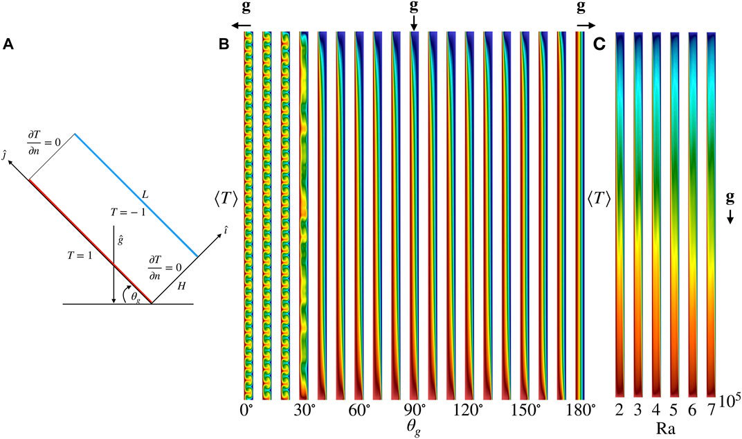
FIGURE 1. (A) Problem configuration. (B) FOM mean (or steady) temperature for 19 uniformly-spaced θg ∈ [0°, 180°] at Ra = 104 and Pr = 7.2. (C) FOM mean temperature for 6 uniformly-spaced Ra ∈ [2 × 10⁵, 7 × 10⁵] at θg = 90° and Pr = 7.2.
Figure 1A illustrates the problem configuration. The aspect ratio is defined as Γ = L/H, where H is the width of the slot and L is the height of the slot. We take H = 1 and L = 40 throughout the study. With θg = 0° the flow corresponds to standard Rayleigh-Bénard convection, 90° corresponds to vertical slot convection, and θg = 180° leads to a pure conduction solution with the cold side on the bottom of the horizontal slot. The Rayleigh and Prandtl numbers are
where ρ is the fluid density, β is the thermal expansion coefficient, ΔT = 2 is the wall-to-wall temperature difference, H is the gap width, g is the gravitational acceleration, ν is the kinematic viscosity, and α is the thermal diffusivity. Figure 1B illustrates representative mean (or steady) temperature fields for 19 uniformly-spaced θg ∈ [0°, 180°] at Ra = 104 and Pr = 7.2. Figure 1C shows the mean temperature field for 6 uniformly-spaced Ra ∈ [2 × 10⁵, 7 × 10⁵] at θg = 90° and Pr = 7.2. The configuration has many interesting applications. For example, it represents energy-efficient double-glazed windows, in which the sealed air gap between the two panes acts as an added layer of insulation. Finding the optimum angle θg that enhances the heat transfer is an important question. Convection in a tilted fluid layer is also of meteorological and oceanographic interest. More information on the impact of θg and Γ on heat transport and flow organization for this configuration can be found in [12].
There has been significant work on pMOR development for the steady Boussinesq equations, including rigorous error estimation [10, 11, 13–15]. For pMOR, the steady problem is easier than the unsteady problem for several reasons: 1) rigorous error estimates are usually achievable, 2) there is often a well defined attractor, and 3) no temporal instability needs to be considered. Once the problem becomes unsteady many open research issues remain. To our knowledge, there are few pMOR works addressing the unsteady parameterized Boussinesq equations. In [16], the authors develop rigorous a posteriori error bounds applied to a 2D Rayleigh-Bénard problem parameterized with Gr and θg. However, due to exponential instability in time, the rigor is not for very high Gr and large final times. In [17], the authors overcame the high Gr issue by considering a space-time formulation which enabled effective long-time certification of a reduced basis approximation of noncoercive PDEs. However, the approach is limited due to large offline computational effort since only one snapshot is generated from one FOM solve due to the formulation. For example, to cover the parameter space, 125 FOMs are solved during the offline in their case.
Fick et al. [9] developed a POD-hGreedy pMOR to study challenging incompressible flow using a time-averaged error indicator. The authors showed that the error indicator is highly-correlated with the error in mean flow prediction and can be efficiently computed through an offline/online strategy. We view the methodology as having high potential for routine analysis and design of turbulent flows that are characteristic of thermal hydraulic systems. Hence, we explore that approach here by extending the time-averaged error indicator to accommodate the energy equation. In previous work [18] on ROM stabilization and turbulent thermal transport problems, we investigated the performance of pMOR with constrained stabilization [9], and Leray regularization [19]. Here, we extend the error indicator to support Leray regularization. For each approach, we assess the performance through the mean flow and QOIs including, mean Nusselt number (Nu), standard deviation in Nu, mean temperature fluctuation and mean turbulent kinetic energy (TKE)1.
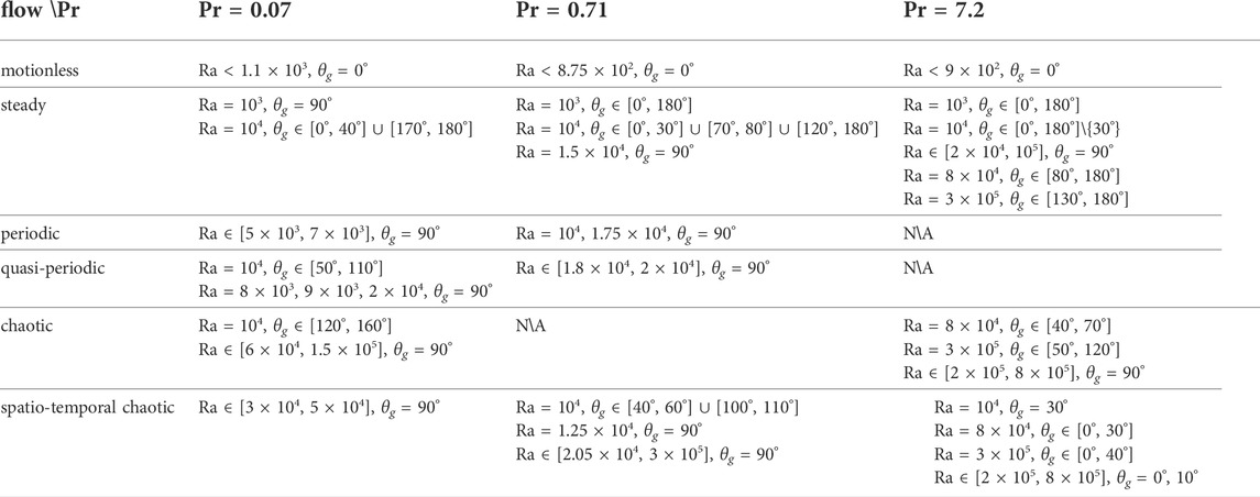
Even though our 2D model problem generates only laminar flows, pMOR is quite challenging in this application for several reasons: 1) there is bifurcation in θg parameter space; 2) the solution can be multivalued, even at steady state; and 3) the solution exhibits spatio-temporal chaos at several points in the parameter space. As our initial efforts happened to be focused in one of the spatio-temporal chaos regimes, we decided to map out a larger space to identify where pMOR could succeed, where it would have difficulty, and where it a priori could not succeed. Table 1 reflects a broad range of flow regimes identified inside the high-aspect ratio slot from hundreds of FOM simulations conducted at multiple Ra, θg with Pr = 0.07, 0.71, 7.2. We categorize the flow into six types: 1) motionless, 2) steady, 3) periodic, 4) quasi-periodic, 5) chaotic and 6) spatio-temporal chaotic. We identify the flow regimes by examining the (mean) solution field and the energy and Nu histories. Such analysis can readily distinguish the motionless, steady and periodic flow cases. Even though the energy and Nu analysis seem to be a reliable way to distinguish the quasi-periodic and chaotic flow, it is only a heuristic—a more rigorous analysis is through computing the power spectrum of Nu or energy [20]. Tools such as Lyapunov exponent and fractal dimension are probably the most widely used diagnostic for chaotic systems [21, 22]. The first five types of low have consistent mean flow in differing time windows, each averaged over 500 convective time units (CTUs). We define a flow to be spatio-temporal chaotic [23] if its mean solution is not consistent in at least three different time windows. This type of flow has strong irregularities in both space and time and has been observed in Rayleigh Bénard convection and in other complex dynamical systems [24]. To characterize spatio-temporal chaos, one could also consider Lyapunov exponents at each grid point. A detail analysis of spatio-temporal chaos is beyond the scope of this paper. A comprehensive review on this topic can be found in [25].
In the present work, we start with solution reproduction problem, which represents the first step towards the development of a ROM for the parametric problem. We study the reproduction capability of the FOM, ROM and ROM with stabilization for the six types of flow reported in Table 1. We report only the cases of chaotic and spatio-temporal chaotic flow. Notice that it has been reported that ROM can often capture the first five types of flow accurately, in some cases, with the need of stabilization methods. However, for the spatio-temporal chaotic flow, to our knowledge, it has not been studied. We believe this is the first work investigate ROM’s reproducibility of spatio-temporal chaotic flow.
The pMOR development is broken into several parametric problems. We start with a problem at Ra = 103 and Pr = 7.2 in which the solution is steady for all θg but nonetheless exhibits a bifurcation at θg = 20°2. We find either h- or p-Greedy with the error indicator based on the dual norm of the residual is able to drive pMOR successfully3. We next consider two sets of parametric problems: 1) problem parameterized with θg at higher Ra. 2) Problem parameterized with Ra. In the first set, similar to the steady case, a bifurcation is observed and the solution space is a blend of steady and unsteady solutions. In the second set, no bifurcation is observed and the solutions are all unsteady.
By proceeding in this manner, we are able to isolate several difficulties and eventually come up with an important observation for the pMOR: Accurate prediction
The paper is organized as follows. In Section 2, we introduce the model problem and governing equations. In Section 2.1, we introduce the Galerkin formulation for the FOM. The ROM, as well as Leray regularization is introduced in 2.2. In Section 3, we consider the solution reproduction problem and assess the numerical performance. The parametric problem is discussed starting from Section 4. We first introduce POD-hGreedy algorithms in Section 4.1 with some remarks on applying POD-pGreedy to this model problem at the end of the section. We then introduce the time-averaged error indicator with thermal extension in Section 4.2. A straight-forward integration with Leray regularization is also shown in the same section. In Sections 4.3 and 4.4, we present the pMOR results with θg variation and Ra variation. In Section 5, we discuss the spatio-temporal chaos and multiple states issues found in this model problem. Finally, we conclude the paper in Section 6.
2 A parametrized natural convection problem
We start with the Boussinesq equations for buoyancy-driven flow [26],
where u is the velocity, p is the pressure, T is the temperature and g(θg) is the unit vector represents the direction of the buoyancy force and it is defined by
In our non-dimensional setting, we set ν = (Pr/Ra)1/2 and α = (Pr Ra)−1/2. The Rayleigh number, Ra = ρβgH3ΔT/(να), represents the ratio of buoyancy force to thermal and momentum diffusive force The Prandtl number Pr = ν/α, reflects the relative importance of momentum diffusivity compared to thermal diffusivity. With this nondimensionalization the characteristic velocity is
For unsteady problems, the QOIs are the mean flow, mean Nu, standard deviation in Nu, mean TKE and mean temperature fluctuation. The symbol ⟨⋅⟩ is used to indicate a time-averaged quantity. The mean velocity and temperature field are defined as:
with tj = jΔt and Δt being the time step. The selection of J0 is based on when the solution reaches it statistically steady state. The mean quantities are then averaged over 500 CTUs, with the time scale defined above. The instantaneous Nusselt number is defined as
with
The mean TKE and mean temperature fluctuation are defined as
For steady problems, the QOIs are simply the steady solutions to Eqs. 2 and 3 and the corresponding Nu using Eq. 5.
2.1 Galerkin formulation for the full-order model
The FOM is constructed through the spectral element method (SEM) and the Pq–Pq−2 velocity-pressure coupling [27], where the velocity is represented as a tensor-product Lagrange polynomial of degree q in the reference element
For any u(x, t), we have a corresponding vector of basis coefficients
with ϕj(x) the underlying spectral element basis functions spanning the FOM approximation space,
Here,
Both the FOM and ROM are cast within the same Galerkin framework. To begin, we introduce several inner products for elements in the FOM space,
Further, for S,
For the FOM, we consider the (semi-discrete) weak form of Eqs. 2 and 3 [29], Find
Here, we have introduced
Following [30], we consider a semi-implicit scheme BDFk/EXTk to discretize Eqs. 13–15 in time; kth-order backward differencing (BDFk) is used for the time-derivative term, kth-order extrapolation (EXTk) is used for the advection and buoyancy terms and implicit treatment on the dissipation terms. As discussed in [30], k = 3 is used to ensure the imaginary eigenvalues associated with skew-symmetric advection operator are within the stability region of the BDFk/EXTk time-stepper. Denoting the solution at time tn = Δt ⋅ n as
Equations 16–18 represent a linear unsteady Stokes plus unsteady heat equation to be solved at each time-step tn. The inhomogeneous terms comprise the BDF, advection, buoyancy and lifting terms
Here, the βss and αss are the respective sth-order BDF and extrapolation coefficients for the BDFs/EXTs time-stepper [30]. Note that the right-hand side of Eq. 17 will be zero if u0 is divergence free or at least satisfies the weak divergence-free condition Eq. 14.
Under the assumption that ∇ ⋅u0 = 0, the compact matrix form [27, 31, 32] for Eqs. 16–20 is
Here,
with
where g1 = cos(θg) and g2 = sin(θg) represent the parametric forcing. The thermal load in Eq. 22 is
Entries of the respective stiffness, mass, convection, and gradient matrices are
Note that {ϕi(x)} forms the spectral element velocity/temperature basis while {ψi(x)} constitutes the pressure basis.
2.2 Galerkin formulation for the reduced-order model
Within the Galerkin framework of the preceding section it is relatively straightforward to develop a ROM. One defines a set of functions
For the ROM, we insert the expansions Eq. 30 into Eqs. 13–15 and require equality for all (v, S) in
The matrix form for the ROM is readily derived by constructing a pair of rectangular basis matrices, B and B, having entries
where the xis are the spectral element nodal points. The coarse-system matrices are Hc,ν = BTHB and Hc,α = BTHαB and the governing system for the ROM becomes
We refer Eq. 32 as Galerkin ROM (G-ROM) throughout the paper. The ROM coefficient vectors,
which follows from the fact that the columns of B and B are, respectively, A- and A-orthonormal, where A = block-diagonal(A). To recover the spectral element representation, we simply prolong the N-length vectors
The functional representations,
Next we consider the Galerkin ROM with Leray regularization using a spatial filter, following ideas presented in [19]. The approach simply requires regularizing the advecting field in the Navier-Stokes equations and energy equation through a low-pass filter function F (i.e.,
The formulation of G-ROM with Leray regularization is shown in Eq. 35 and the only difference comparing to G-ROM Eq. 32 are the velocity data and thermal load.
where
and
In this work, we will be focusing on a PDE- (or differential-) based filter, which is characterized by a filter width, δ [35]. Following [19, 36], such filters are developed in a POD context as follows: Find
Besides the differential filter, one could also consider a more economic spatial filter, namely, a POD-projection (Proj) filter as discussed in [19]. In this case, one simply truncates the higher POD mode contributions when constructing
Besides G-ROM and LDF-ROM, we also consider the constrained-evolution stabilization introduced in [9]. The idea behind this approach is to use information from the snapshot set to establish a priori limits on the ROM coefficients
where the constraints mj and Mj on the basis coefficients
3 The solution reproduction problem
In this section, we consider the solution reproduction problems for Ra = 2 × 10⁵, 7 × 10⁵ at Pr = 7.2 and θg = 90°, where the solutions are chaotic. We assess the performance of G-ROM, C-ROM and LDF-ROM introduced in Section 2.1 through the accuracy of the mean field and the QOIs. The mean field is computed by averaging the POD coefficients and reconstructing with the rectangular basis matrices B and B. The QOIs are the mean Nu and Std(Nu), which are estimated through Eq. 6, and the mean TKE and mean temperature fluctuation, estimated through Eq. 7. The quantities are averaged over 500 CTUs.
Although of limited practical interest, the solution reproduction problem is an important step towards the development of a MOR procedure for the parametric problem. The reproduction results for spatio-temporal chaotic flow are presented and discussed in Section 5.1.
3.1 Numerical results
Results for Ra = 2 × 10⁵ are shown in Figures 2A–D. The performances of G-ROM, C-ROM and LDF-ROM are indicated by blue, orange, green solid line. In LDF-ROM, the radius of the differential filter is δ = 0.015625. Figure 2A shows the behavior of the relative
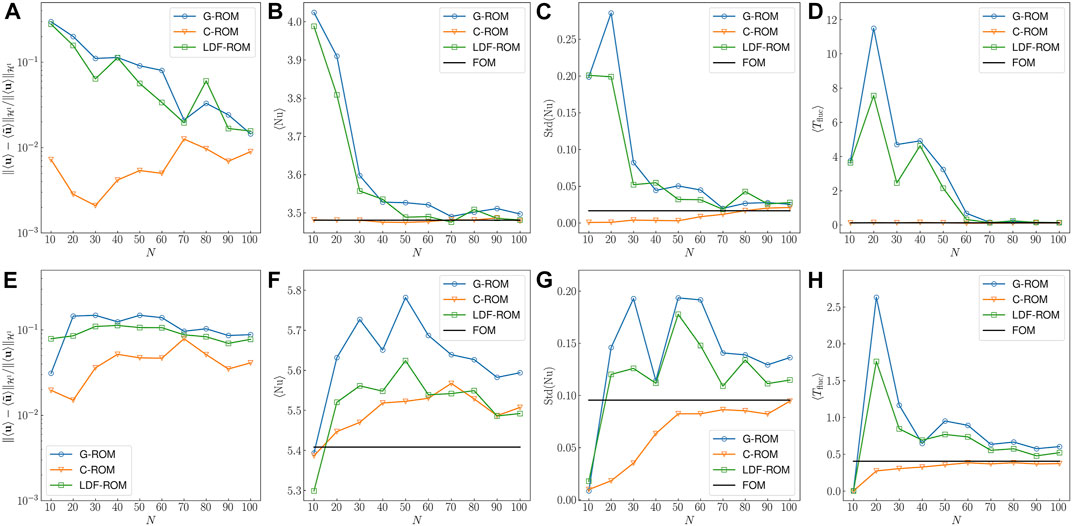
FIGURE 2. Performance comparison between G-ROM, C-ROM and LDF-ROM for the solution reproduction problem at θg = 90° and Pr = 7.2. (A–D) Behavior of the relative
Note that the differential filter radius δ selected for the two Ra yields the best accuracy in mean flow among the five differential filter radius δ = 0.25, 0.125, 0.0625, 0.03125, 0.015625. Besides, we find δ = 0.015625 yield the best results at smaller Ra and as Ra increases, results with δ = 0.03125 becomes better and are comparable with δ = 0.015625 at Ra = 7 × 10⁵. The tendency is reasonable since the flow is more chaotic as Ra increases, therefore one should expect a larger δ to stabilize the flow.
From the results, we observe the mean flow and QOIs converge with N for all ROMs. With higher Ra, convergence in those quantities is much slower and a larger N is required to reach to the same accuracy as in the lower Ra case. Note that, because of the O(N3) online costs, requiring a large value of N for convergence might require off-line resources for timely simulation, which would greatly diminish the intrinsic advantage of the ROM/pMOR framework. This potentiality highlights the importance of stabilization methods. Indeed, we find that C-ROM is able to predict the mean flow and QOIs with a better accuracy with smaller N. On the other hand, although LDF-ROM is not as effective as C-ROM, and only slightly better than G-ROM, it will play a key role in the pMOR presented in Section 4, especially in the parametric problem with θg variation.
4 The parametric problem
We turn now to study the performance of pMOR for the slot problem with G-ROM, C-ROM, and LDF-ROM. Two sets of parameterization are considered. With Pr = 7.2 fixed, we seek to estimate the solution and QOIs of Eqs. 13 and 15 for: 1)
For efficient selection of the pMOR anchor points we consider the POD-hGreedy algorithm proposed in [9] which combines POD in time with Greedy in parameter. The term Greedy refers to the optimization strategy of basing anchor point selection on the training point that exhibits the largest value in the error estimate. Error-indicated selection of the anchor points reduces the number of FOM solves and is thus critical for the feasibility of pMOR. Here, the error indicator corresponds to the dual norm of the residual associated with the time-averaged momentum and energy equations.
The section is organized as follows. In Section 4.1 we present the POD-hGreedy algorithm. In Section 4.2, we extend the time-averaged error indicator introduced in [9] to accommodate the energy equation and Leray regularization. Finally, in Sections 4.3 and 4.4, we present the numerical results.
4.1 Proper orthogonal decomposition-hGreedy algorithm
In this section, we present the POD-hGreedy algorithm for the construction of the reduced spaces
To begin, we introduce the discretized parameter space
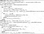
Algorithm 1 presents the computational procedure for both offline and online stage. The offline procedure starts with an anchor point that could either be selected randomly from the training space
Given the ROM/anchor point data
Algorithm 1. POD-hGreedy algorithm for the construction of
1) The reduced bases are shared between anchor points. POD is still used to construct the new basis but the collected snapshot set is projected onto the orthogonal complement of the existing basis.
2) In the online/training stage, only one ROM is used instead of a set of ROMs and there is no need to check for the nearest anchor points.
3) The anchor point is selected based on the single error estimate Δ in current iteration, rather than the individual estimates for each ROM.
Although it has a better convergence rate than POD-hGreedy, POD-pGreedy can easily fail for unsteady problems. Combining modes at different anchor points, especially ones whose solution exhibits different physics, can easily lead to instability and deteriorate the performance, as noted in [9]. Moreover, stabilizations that work for POD-hGreedy can fail in the POD-pGreedy approach. For example, in C-ROM, it is not clear how to construct the constraints for the combined basis. A naive approach is to apply POD to all the snapshots at anchor points. However, this approach is inefficient and can be limited by the computer storage requirements during the offline phase. Leray regularization with the projection filter (i.e., trivially truncated basis set for the advector) is also limited since the combined basis is no longer ordered in a Fourier-like, energy-decaying, sequence. To address this, one could apply POD to all the snapshots that have been collected but this approach is again limited by the storage and therefore not practical. An alternative is to consider DF filter, denoted as LDF-ROM here. Once the radius δ is specified, it will filter right amount of energy in each basis.4.2 A time-averaged error indicator
In this section, we extend the time-averaged error indicator proposed in [9] to accommodate the energy equation and Leray regularization. The error indicator is based on the dual norm of the discrete time-averaged residual. Given the ROM solution sequence
where
Note for simplicity, we assume only BDF3/EXT3 is used for time discretization in Eqs. 42 and 43. Besides, the residual is defined over
We define the time-averaged error indicator,
The residuals Eqs. 42 and 43 can be further expressed in the matrix-vector form since the spaces
The matrix-vector version of the discrete time-averaged residual Eqs. 40 and 41 is then expressed as
Thanks to the Riesz representation theorem, there exist a unique
It thus follows that
Equations 51 and 52 allows one to compute the Riesz representers
In practice, determination of the Riesz representers,
Here, A corresponds to H introduced in Eq. 23 with β0 = 0 and ν = 1. We remark that the essential difference between the velocity and temperature representers is that the former satisfies the divergence-free constraint by virtue of the 2 × 2 block system in Eq. 55. Evaluation of the error indicator Δ entails solving Eqs. 55 and 56, computing the corresponding
While use of the direct approach requires access to the FOM machinery in order to generate an error indicator, we note that such access is readily available during the pMOR training/construction phase. The advantage of this approach is that the number of Stokes/Poisson solves scales as the number of points in the training space, which is typically less than N2. The other is through the offline/online computational decomposition which takes the advantage of the affine decomposition and expands the residual. By expanding the residuals ⟨Ru⟩ and ⟨RT⟩, 2(N + 1)2 + 6(N + 1) linear functionals are derived, where 2(N + 1)2 is due to the convection term in the Navier-Stokes and energy equations. Applying the Riesz representation theorem to each linear functional, we end up solving 2(N + 1)2 + 6(N + 1) Riesz representers, where (N + 1)2 + 4(N + 1) of them are solved through Stokes problems and (N + 1)2 + 2(N + 1) of them are solved through Poisson problems. Note that the Riesz representers must be stored in order to accomplish the decomposition and each is a vector of size
4.2.1 Time-averaged error indicator with Leray regularization
The integration of the time-averaged error indicator Δ with Leray regularization is rather straightforward. Recall the difference between G-ROM Eq. 32 and LDF-ROM Eq. 35 is simply the advecting field being filtered. Hence, the residuals
for all
4.3 Parametric model order reduction results: θg variation
In this section, we consider the parametric problem parameterized with θg at Pr = 7.2. The problem has three characteristics: bifurcation, spatio-temporal chaos over a certain range of θg, and a solution manifold that is a blend of steady and unsteady solutions. To identify the major pMOR challenges for this case, three values of Ra are considered:
1) Ra = 1 × 10⁴ where the FOM is steady except at θg = 30°.
2) Ra = 8 × 10⁴ where the FOM is unsteady for θg ∈ [0°, 70°] and steady for θg ∈ [80°, 180°].
3) Ra = 3 × 10⁵ where the FOM is unsteady for θg ∈ [0°, 120°] and steady for θg ∈ [130°, 180°].
In each case, the ROM is constructed through Algorithm 1. In order to assess performance, we generate FOM data for θg = 0°, 10°, …, 180° (ntrain = 19 datapoints). The FOM solution is obtained by solving Eqs. 2 and 3. For parameters where the problem is steady, the solution and the Nu are collected after the solution difference between ten time steps is less than 10–6. For unsteady problems, the mean flow, mean Nu, Std(Nu), mean TKE and mean temperature fluctuation are averaged over 500 CTUs after the solution has reached a statistically steady state.
Although not shown here, we remark that at Ra = 1 × 10³, the problem is steady with a bifurcation at θg = 20°. In this case, either h- or p-Greedy with residual dual-norm base error indicator accurately estimates the solution and QOIs over the parameter space θg ∈ [0°, 180°].
4.3.1 Ra = 1 × 10⁴
To examine the feasibility of the pMOR (Algorithm 1) in the unsteady case, we begin with Ra = 1 × 10⁴, in which only one unsteady solution is introduced at θg = 30°.
Figure 3E shows the steady (or mean) velocity magnitude for 19 uniformly-space training points θg = 0°, 10°, …, 180°. The corresponding temperature distributions are in Figure 1B. At θg = 180°, we observe no flow and the temperature is simply the conduction solution. As θg decreases, we observe slot convection and then about θg = 40° there is a bifurcation to the wavy flow and rolls in the velocity. Moreover, we observe spatial-temporal chaos at θg = 30°. Figures 3A–D show the results of the application of Algorithm 1 for the construction of the G-ROM, C-ROM and LDF-ROM for the pMOR. The algorithm starts with
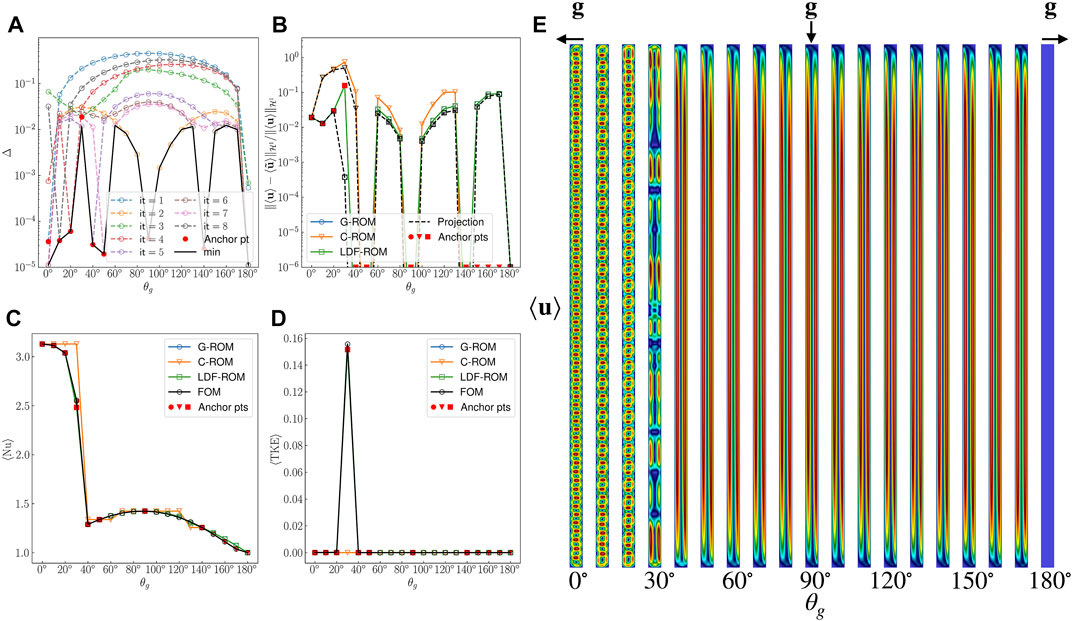
FIGURE 3. POD-hGreedy performance comparison between G-ROM, C-ROM and LDF ROM for the parametric problem parameterized with θg at Ra = 1 × 10⁴ and Pr = 7.2. (A) Behavior of the error indicator Δ defined in Eq. 44 for eight iterations with G-ROM. (B–D) Behavior of the relative
Figure 3A demonstrates the selection process of anchor points (denoted by red circles) for the G-ROM case. We briefly walk through the process: At the first iteration, the error estimate Δ1(θg) for
From Figure 3A, we observe the error estimate is small at anchor points where the problem is steady. On the other hand, although the error estimate Δ3(θg) (greed line) is small at
Following this procedure for the other cases, we present models results for the G-ROM, C-ROM and LDF-ROM cases, denoted respectively blue, orange, green solid lines in Figures 3B–D. The behavior of the relative
Before closing this section, we highlight some observations with respect to the solution manifolds.
1) The solutions at θg ∈ [0°, 30°] are Rayleigh-Bénard with differing numbers of rolls, analogous to orthogonal sine and cosine functions at different wave numbers. Therefore, there is little hope in reproducing the solution except at selected anchor points. QOI’s such as mean Nu, however, are less sensitive to precise mean flow fields and are therefore more tractable.
2) At θg = 170° and θg = 180° the thermal metrics are not too different despite the
The first issue is resolved by the error indicator picking θg ∈ [0°, 30°] as anchor points. The second issue can be a source of error as Ra increases. With θg = 160° as an anchor point and the solution at θg = 180° as the lift function, the error at θg = 170° is 9% for Ra = 1 × 10⁴, 16% for Ra = 8 × 10⁴, and 19% for Ra = 3 × 10⁵.
4.3.2 Ra = 8 × 10⁴
Figure 4 shows pMOR results analogous to Figure 3 for the case Ra = 8 × 10⁴. Here, we consider only the G-ROM and LDF-ROM. The algorithm starts with
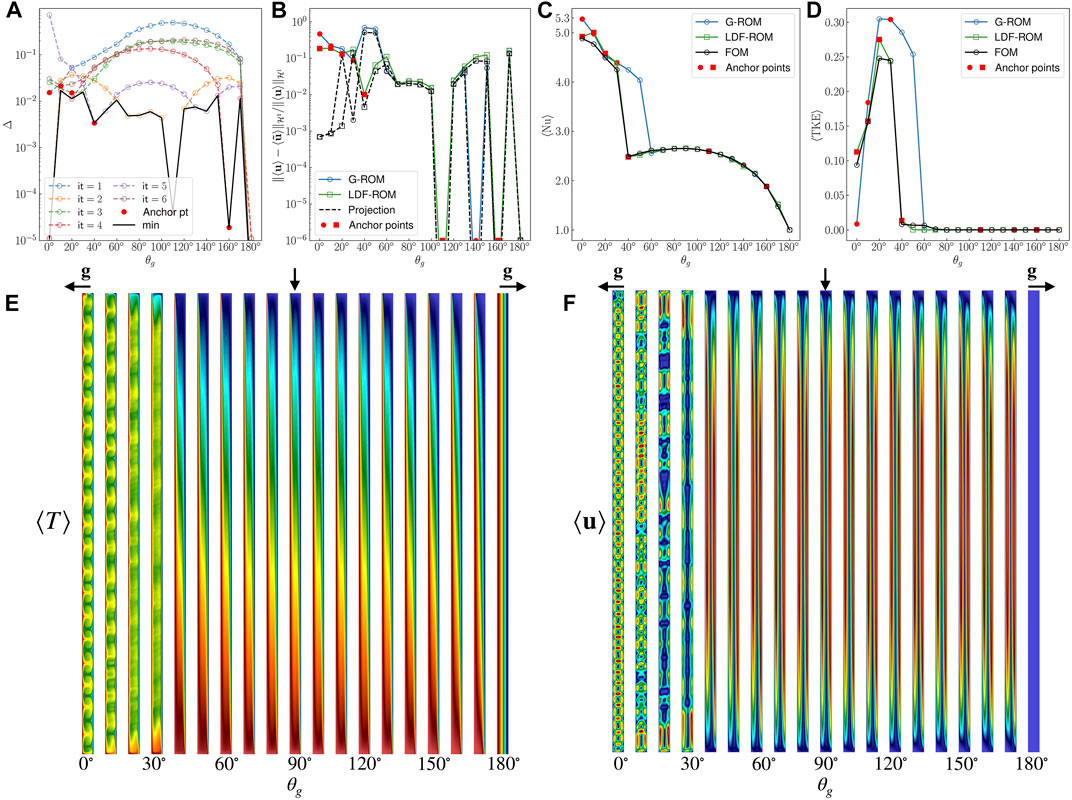
FIGURE 4. POD-hGreedy performance comparison between G-ROM and LDF ROM for the parametric problem parameterized with θg at Ra = 8 × 10⁴ and Pr = 7.2. (A) Behavior of the error indicator Δ defined in Eq. 44 for six iterations with LDF-ROM. (B–D) Behavior of the relative
The anchor-point selection process with LDF-ROM is demonstrated in Figure 4A. Starting with
The behaviors of the relative
The behavior for mean Nu and mean TKE are shown in Figures 4C,D for G-ROM and LDF-ROM. Despite large errors in the mean flow prediction at θg = 0°, 10°, the LDF-ROM is able to predict mean Nu with a maximum error around 5% whereas G-ROM has maximum error around 28%. In addition, LDF-ROM is able to more accurately predict mean TKE than G-ROM.
4.3.3 Ra = 3 × 10⁵
For (Pr,Ra) = (7.2, 3 × 10⁵) the flow is quite chaotic (similar to what is found for Pr = 0.71 at lower Ra). Figures 5E,F show the mean (or steady) temperature and velocity solution at θg = 0°, 10°, …, 180° (19 datapoints). This time, the bifurcation occurs at θg = 60°. We use this elevated Rayleigh-number case to explore the behavior of the h-Greedy pMOR convergence by considering application of the algorithm to two different training sets,
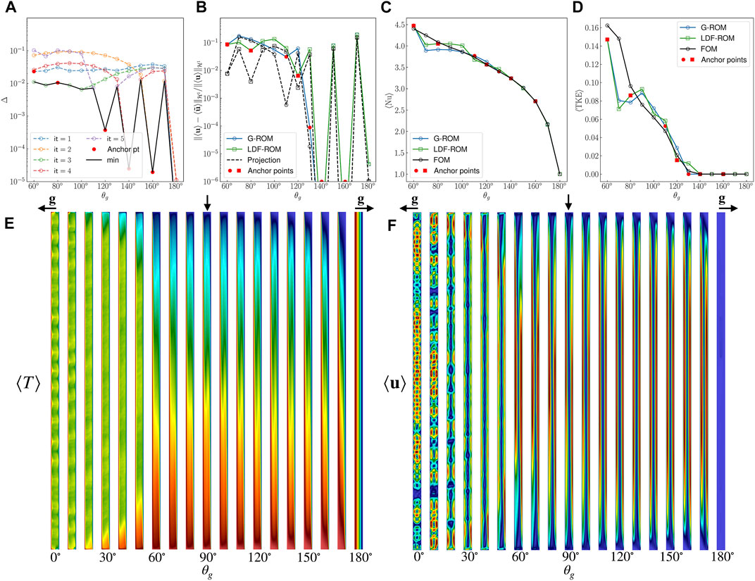
FIGURE 5. POD-hGreedy performance comparison between G-ROM and LDF ROM for the parametric problem parameterized with θg ∈ [60°, 180°] at Ra = 3 × 10⁵ and Pr = 7.2. (A) Behavior of the error indicator Δ defined in Eq. 44 for five iterations with LDF-ROM. (B–D) Behavior of the relative
The anchor point selection process for
The behavior of the mean Nu and mean TKE are shown in Figures 5C,D. The maximum error in the predicted mean Nu is around 5% with LDF-ROM and 8% with G-ROM. The mean TKE estimation is also reasonable but is underestimated at θg = 70°.
Next we examine the same problem configuration but with the full parameter space

FIGURE 6. POD-hGreedy performance comparison between G-ROM and LDF ROM for the parametric problem parameterized with θg ∈ [60°, 180°] at Ra = 3 × 10⁵ and Pr = 7.2. (A) Behavior of the error indicator Δ defined in Eq. 44 for five iterations with LDF-ROM. (B–D) Behavior of the relative
The relative
We are also aware that in some applications, the Std(Nu) could be considered as QOI. However, comparing to the mean Nu and mean TKE, we find Std(Nu) is in general a more challenging QOI. Figure 7 shows the predicted Std(Nu) in the three Ra cases. We observe accurate prediction in Ra = 1 × 10⁴ case. However, unlike the mean TKE, the Std(Nu) soon becomes intractable with Ra = 8 × 10⁴ even with Leray regularization and is even worse in Ra = 3 × 10⁵.

FIGURE 7. Behavior of the predicted Std(Nu) with θg. (A): G-ROM, C-ROM and LDF-ROM estimation at Ra = 1 × 10⁴ with eight anchor points. (B): G-ROM and LDF-ROM estimation at Ra = 8 × 10⁴ with six anchor points. (C): G-ROM and LDF-ROM estimation at Ra = 3 × 10⁵ with six anchor points.
4.4 Parametric model order reduction results: Ra variation
In this section, we consider the slot problem at θg = 90° and Pr = 7.2 with the parametric space defined by
Figure 8 shows the results of the application of Algorithm 1 for the pMOR using G-ROM, C-ROM and LDF-ROM. The solid line denotes the performance of the reduced model which minimizes the error indicator, and thus is selected by the Greedy procedure (cf. Algorithm 1, ncand = 2). Anchor points are denoted as red circle while FOM data is denoted as black solid line. The algorithm starts with

FIGURE 8. POD-hGreedy performance comparison between G-ROM, C-ROM and LDF ROM for the parametric problem parameterized with Ra at θg = 90° and Pr = 7.2. (A–D) Behavior of the relative
Figure 8A shows the behavior of the relative
Figure 8B shows the behavior of the predicted mean Nu with Ra. At the anchor points, we observe good agreement between ROMs and FOM and that stabilization does improve its accuracy. The maximum relative error is roughly 8% in G-ROM, 6.5% in C-ROM and 5% in LDF-ROM. Figures 8C,D show the behavior of the predicted Std(Nu) and mean temperature fluctuation. In both QOIs, we find C-ROM outperforms the other two models. At Ra = 7 × 10⁵, LDF-ROM is only slightly better than G-ROM.
This parametric space is in general more tractable than those involving variation in θg. This outcome might be anticipated by observing the mean temperature fields shown in Figure 1C, which suggests that the solution manifold with respect to Ra is quite smooth. This is also reflected in the QOIs, for example, the mean Nu, Std(Nu) and mean temperature fluctuation behave almost linearly as Ra increases.
5 Discussion
In this section, we investigate some of the flow behaviors exhibited by the FOM to better understand how they influence the relative performance of the ROMs. We note that we cannot, in general, expect a ROM to be able to predict FOM behavior if the flow itself is not predictable. Thus, variability in the FOM provides an anticipated lower bound on ROM performance for the reproduction problem.
5.1 Spatio-temporal chaos
As pointed out in the introduction, we classify a flow to be spatio-temporal chaotic by examining its consistency in mean flow over various time windows. (We use this simple metric here for convenience—we have also examined the flow fields and the time traces of multiple QOIs.) Here, we explore how lack of consistency influences four QOIs, mean Nu, Std(Nu), mean temperature fluctuation, and mean TKE, at three successive time windows, W1, W2 and W3. These quantities are used to indicate the variability in the FOM. As with the preceding cases, we consider averaging times of 500 CTUs for each of the three windows. The starting time for W1 differs with given parameters as some cases take a longer time to reach a statistically steady state. For example, for Pr = 0.71 at Ra = 1.8 × 10⁴ and θg = 90°, the flow is chaotic until 6,000 CTUs and then becomes periodic.
Figures 9A–D show the behavior of the four QOIs with Ra at three Pr for θg = 90°. Pr = 0.07 is denoted as green line, Pr = 0.71 is denoted as orange line, while Pr = 7.2 is denoted as blue line. Window W1 is denoted by a solid line, W2 by a dashed line, and W3 by a dotted line.
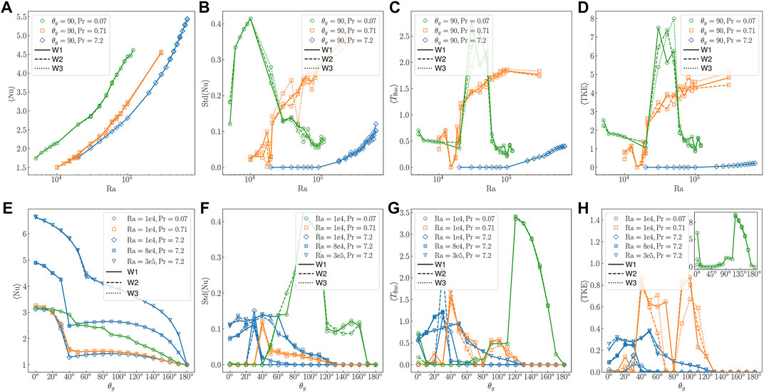
FIGURE 9. Parametric variability in the FOM: green–Pr = 0.07, orange–Pr = 0.71, and blue–Pr = 7.2. Each plot reveals absence/presence of chaotic effects by presenting statistics taken over three time windows, W1, W2, and W3. (A–D): Ra-dependence of mean Nu, Std(Nu), mean temperature fluctuation, and mean TKE computed over time windows W1, W2 and W3. (E–H): θg-dependence at fixed Ra.
From Figures 9A–D we can see the following:
1) For Pr = 0.07 the QOIs are fairly consistent except for Ra ∈ [3 × 10⁴, 5 × 10⁴].
2) For Pr = 0.71, we find large variability in Std(Nu), mean temperature fluctuation and mean TKE for Ra > 2 × 10⁴.
3) Pr = 7.2 exhibits the least variability.
For Ra where we find that the QOI variability is high, we have also examined the mean flow at multiple time windows and found that those are also inconsistent. In all cases, the mean Nu is quite repeatable.
Figures 9E–H show the behavior of the same QOIs as a function of θg. For Pr = 7.2, we consider three different values of Ra. We find for most of the θg, the variability is small except for small θg where we also report spatio-temporal chaotic flow. For Pr = 0.07, we find the QOIs has small variability with Ra = 1 × 10⁴. However, for Pr = 0.71, we find large variability, especially in the mean TKE. Not only it has spatio-temporal chaotic flow (for example θg = 100°), but also the solution manifold is not smooth. By varying θg = 80° to θg = 100°, the solution changes from steady to periodic then spatio-temporal chaotic.
From Figures 9E–H we observe the following:
1) For Pr = 0.07, Std(Nu) exhibits up to 50% variability (e.g., at θg = 70°) while ⟨Tfluc⟩ and ⟨TKE⟩ have orders-of-magnitude relative variability at θg = 0°.
2) For Pr = 0.71, ⟨Tfluc⟩ and ⟨TKE⟩ exhibit significant variability for θg ∈ [60°, 110°].
3) For Pr = 7.2, the most notable variation is at θg = 30° for Std(Nu), ⟨Tfluc⟩, and ⟨TKE⟩ at Ra = 104. Remarkably, the higher Rayleigh number cases do not exhibit as much variance.
As in Figures 9A–D, the mean Nu is seen to be a repeatable QOI. It is worth noting the real challenge and sensitivity of this class of problems is illustrated in Figure 9H. Here, we observe for the (Pr, Ra) = (0.71, 104) case that the flow alternates from steady to unsteady at multiple points along the one-dimensional θg parameter space as indicated by several distinct zeros in the TKE.In Figure 10, we further explore the influence of spatio-temporal chaos by examining the mean-flow distributions and ROM performance for (Pr, Ra) = (7.2, 3.5 × 10⁴) at θg = 0° and θg = 20°. Figures 10A–C show the behavior of the
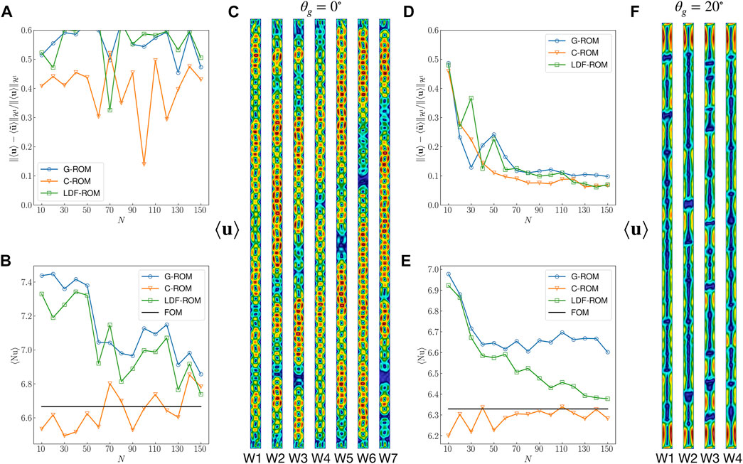
FIGURE 10. ROM performance comparison between problem having significant (θg = 0°) and less significant (θg = 20°) spatio-temporal chaotic flow at Pr = 7.2 and Ra = 3 × 10⁵. (A–C) Behavior of the relative
We have also computed the relative error between FOM mean flows across seven time windows for the two values of θg. The maximum relative
In Figure 11, we examine the influence of Prandtl number by comparing results for Pr = 0.71 and 7.2 at (Ra, θg)= (3 × 10⁵, 90°). Figures 11A–D show the convergence behavior for the
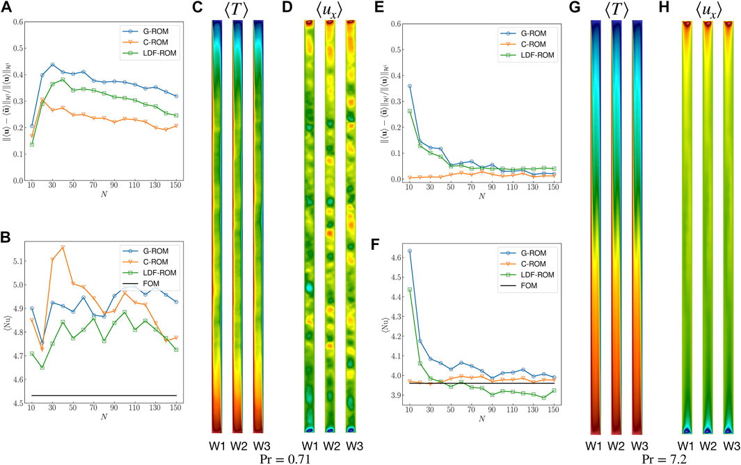
FIGURE 11. ROM performance comparison between Pr = 0.71 and Pr = 7.2 at Ra = 3 × 10⁵ and θg = 90°. (A–D) Behavior of the relative
In summary, the results of this section show that convergence issues and variations in the QOIs in the ROM can have high a correlation with the flow being spatio-temporal chaotic. From Table 1 and Figure 9, we see that Pr = 0.71 has a more complicated solution manifold found with the other two Prandtl numbers and also exhibits spatio-temporal chaos at a relatively small Rayleigh number, Ra = 104.
5.2 Multiple steady-state solutions
In this section, we report the existence of multiple steady-state solutions observed for the case (θg, Ra)=(0°, 104). The variations are characterized by different numbers of recirculation rolls, which are induced by using different initial conditions. Figure 12 shows steady temperature solutions generated by starting with steady solutions, χn from other values of θg = n°, save for the χ90 case, which corresponds to a single snapshot of the unsteady flow/temperature field at θg = 90°. Multiple steady states are also observed for this Prandtl number at θg = 10° and 20° and have been reported by other authors as well [12, 14, 40].

FIGURE 12. Different steady temperature solutions at θg = 0°, Ra = 1 × 10⁴ and Pr = 0.71. The solutions were computed from different initial conditions, χn, corresponding to FOM solutions at θg = n°. For n = 2, 10, 20, and 180 the solution is steady, whereas χ90 is simply a snapshot from the θg = 90° case.
For solution reproduction, the multiplicity of the solutions is not an issue as long as the ROM uses the same initial condition as the FOM. However, for parametric problem, these multiple states could easily lead to an incorrect (or at least, unexpected or unverifiable) conclusion. For example, if the ROM anchor at θg = 10° is used to approximate the solution at θg = 0°. With the initial condition at θg = 10°, the approximate solution will be the third temperature solution shown in Figure 12. However, if one collects the FOM data at θg with zero initial condition, one will consider the first temperature solution as the truth solution. As we could consider those roll solutions as sine and cosine functions, the first and third solution are nearly orthogonal; their difference is
5.3 Discussion summary
We have noted in Table 1 the broad range of flow regimes encountered for the tilted slot problem and in this section have illuminated a correlation between the flow states and predictive power of the MOR/pMOR framework. The cases with spatio-temporal chaos are generally the most challenging for model-order reduction and the pMOR errors are found to be (approximately) bounded from below by the variance observed in successive FOM simulations performed at the same parametric point. The development of the pMOR thus needs to be performed with care.
Two parameterizations were considered: 1) θg-variation, where a bifurcation exists and solution space is a blend of unsteady and steady solutions, and 2) Ra-variation, where no bifurcation exists and one finds only unsteady solutions. In the θg-variation problem, accurate prediction in mean flow and other QOIs by the pMOR was demonstrated in the Ra = 1 × 10⁴ and Ra = 8 × 10⁴ cases. In high Ra cases, acceptable prediction of Nu is achieved with LDF-ROM but a small mean-flow error is not realizable because of spatio-temporal chaos.
The results also indicate that the LDF-ROM is a better candidate for parametric problems with bifurcation than C-ROM. This observation is new, yet consistent with the results of [9], where the authors show that C-ROM is effective for parametric problems that do not have a bifurcation. For the parametric problem parameterized with Ra, without spatio-temporal chaos, we find that pMOR with any of the three methods, G-ROM, C-ROM, or LDF-ROM, is able to predict the mean flow quite well. In this case, C-ROM is the most accurate in mean flow prediction and other targeted QOIs. This result is not surprising given that the solution manifold does not have a bifurcation. Lastly, we remark that Std(Nu) is generally the most challenging QOI of those explored here.
From the results, we are able to make an important observation. For parametric problems where pMOR is successful (e.g., errors
Although not shown here, we have also applied POD-pGreedy to this problem. In the parametric problem parameterized with θg, it works only in the steady case Ra = 1 × 10³. Once the unsteady solution emerges, for example at Ra = 1 × 10⁴, combining modes associated with different values of θg leads to an unstable ROM even with the Leray regularization. Although no rigorous proof is given, we hypothesize that the issue is due to the bifurcation in solution behavior. This point was also suggested in [9], which empirically showed that combining modes associated with qualitatively different behaviors might lead to poor prediction. By contrast, when the current problem is parameterized with Ra we find that POD-pGreedy is more efficient than the h-refinement approach.
6 Conclusion
In this paper an error-indicated pMOR is applied to a 2D unsteady natural convection in a tilted high-aspect ratio slot. We first considered the solution reproduction problem (non-predictive case) to demonstrate the convergence of the ROMs and the effectiveness of the stabilization methods. We next addressed the parametric problem (predictive case) to validate the error indicator and, more broadly, the stabilized POD-hGreedy procedures. Principal contributions include, 1) extension of the error indicator proposed in [9] to buoyancy-driven flows; 2) demonstration that Leray-regularized Galerkin ROMs provide a robust solution approach for this class of flows; 3) identification of spatio-temporal chaos as a source of irreproducibility in both the FOM and the ROM and that the variance in the FOM provides a lower bound on the pMOR error in these cases; 4) observation that accurate prediction
We also highlight a number of challenges that are particularly relevant for buoyancy-driven flows and which should be taken into consideration in the design of pMOR strategies for 3D buoyancy driven turbulent flow. First, one needs to be aware of potential convergence issues for the mean flow and other QOI predictions when the FOM exhibits large-scale spatio-temporal chaos. Second, it is difficult to combine modes associated with different flow regimes, especially for the pGreedy case. Third, even relatively simple (e.g., steady) flows can exhibit multiple states at a given parameter. And fourth, there are large offline costs both in terms of computational time and required storage for error indicator and O(N4) costs for online-only error indicators5.
We outline potential next steps in pMOR development for this class of problems.
1) Extension to higher dimensional parameter space. In this work, we considered only one-dimensional parameter space since the pMOR behavior needed to be carefully diagnosed; however higher dimensional parameter spaces are more interesting for engineering applications.
2) hp-Greedy with a bifurcation detection technique. Although we find LDF-ROM is more efficient than C-ROM for parametric problems that have a bifurcation, the h-refinement strategy considered in this paper might require an infeasible number of offline simulations as the dimension of the parameter space increases. To tackle complex parametrizations, more advanced sampling strategies that combine h- and p-refinement [37], potentially with bifurcation detection, could be beneficial [42].
Data availability statement
The original contributions presented in the study are included in the article/Supplementary Material, further inquiries can be directed to the corresponding authors.
Author contributions
P-HT derived the formulation and error indicator, performed the numerical simulations, collected the data, analyzed and interpreted the results. PF supervised the project, provided critical feedback and helped on interpreted the results. Both authors prepared the manuscript.
Funding
This research is supported by the DOE Office of Nuclear Energy under the Nuclear Energy University Program (Proj. No. DE_NE0008780). Simulations were performed at the DOE Office of Science User Facility ALCF (Argonne Leadership Computing Facility).
Acknowledgments
We thank Anthony T. Patera (MIT) for his valuable comments, many contributions, insights and guidelines.
Conflict of interest
The authors declare that the research was conducted in the absence of any commercial or financial relationships that could be construed as a potential conflict of interest.
Publisher’s note
All claims expressed in this article are solely those of the authors and do not necessarily represent those of their affiliated organizations, or those of the publisher, the editors and the reviewers. Any product that may be evaluated in this article, or claim that may be made by its manufacturer, is not guaranteed or endorsed by the publisher.
Footnotes
1Technically, since these flows are not turbulent the TKE should be referred to as velocity variance. Because the is more widely used and the mathematical formulation is the same in either case, we prefer to use the more widely recognized appellation, TKE.
2The ROM coefficients in the steady problems are typically found through a Newton minimization over the POD approximation space [10, 11].
3The pMOR greedy strategy uses the maximal indicated error among the parametric training set to select the next anchor point. p-Greedy combines basis functions from FOMs at different anchor points to form an enriched approximation space; h-greedy builds an independent ROM for each anchor point Ngoc Cuong et al. [10].
4In [16], the velocity and temperature residuals are coupled because the velocity-temperature solutions are obtained through a coupled Newton’s method. Here, we do not couple the residuals because we solve Eqs. 21 and 22 separately.
5The O(N4) costs, which arise from the rank-3 advection tensor, might be mitigated by an O(N2) approximation to the advection operator, such as suggested in [41].
References
1. Grepl MA, Patera AT. A posteriori error bounds for reduced-basis approximations of parametrized parabolic partial differential equations. ESAIM: Math Model Numer Anal (2005) 39:157–81. doi:10.1051/m2an:2005006
2. Rozza G, Huynh DBP, Patera AT. Reduced basis approximation and a posteriori error estimation for affinely parametrized elliptic coercive partial differential equations. Arch Comput Methods Eng (2008) 15:229–75. doi:10.1007/s11831-008-9019-9
3. Merzari E, Ninokata H, Mahmood A, Rohde M. Proper orthogonal decomposition of the flow in geometries containing a narrow gap. Theor Comput Fluid Dyn (2009) 23:333–51. doi:10.1007/s00162-009-0152-3
4. Merzari E, Pointer WD, Fischer P. A POD-based solver for the advection-diffusion equation. Fluids Eng Division Summer Meet (2011) 44403:1139–47.
5. Quarteroni A, Rozza G, Manzoni A. Certified reduced basis approximation for parametrized partial differential equations and applications. J Math Ind (2011) 1:3. doi:10.1186/2190-5983-1-3
6. Wang Z, Akhtar I, Borggaard J, Iliescu T. Proper orthogonal decomposition closure models for turbulent flows: A numerical comparison. Computer Methods Appl Mech Eng (2012) 237:10–26. doi:10.1016/j.cma.2012.04.015
7. Kaneko K, Fischer P. Augmented reduced order models for turbulence. Front Phys (Forthcoming 2022).
8. Quarteroni A, Manzoni A, Negri F. Reduced basis methods for partial differential equations: An introduction. Switzerland: Springer (2015).
9. Fick L, Maday Y, Patera AT, Taddei T. A stabilized POD model for turbulent flows over a range of Reynolds numbers: Optimal parameter sampling and constrained projection. J Comput Phys (2018) 371:214–43. doi:10.1016/j.jcp.2018.05.027
10. Ngoc Cuong N, Veroy K, Patera AT. Certified real-time solution of parametrized partial differential equations. In: Handbook of materials modeling. Dordrecht, Netherlands: Springer (2005). p. 1529–64.
11. Veroy K, Patera AT. Certified real-time solution of the parametrized steady incompressible Navier–Stokes equations: Rigorous reduced-basis a posteriori error bounds. Int J Numer Methods Fluids (2005) 47:773–88. doi:10.1002/fld.867
12. Wang Q, Wan ZH, Yan R, Sun DJ. Multiple states and heat transfer in two-dimensional tilted convection with large aspect ratios. Phys Rev Fluids (2018) 3:113503. doi:10.1103/physrevfluids.3.113503
13. Deparis S. Reduced basis error bound computation of parameter-dependent Navier–Stokes equations by the natural norm approach. SIAM J Numer Anal (2008) 46:2039–67. doi:10.1137/060674181
14. Deparis S, Rozza G. Reduced basis method for multi-parameter-dependent steady Navier–Stokes equations: Applications to natural convection in a cavity. J Comput Phys (2009) 228:4359–78. doi:10.1016/j.jcp.2009.03.008
15. Ballarin F, Rebollo TC, Ávila ED, Mármol MG, Rozza G. Certified Reduced Basis VMS-Smagorinsky model for natural convection flow in a cavity with variable height. Comput Mathematics Appl (2020) 80:973–89. doi:10.1016/j.camwa.2020.05.013
16. Knezevic DJ, Nguyen NC, Patera AT. Reduced basis approximation and a posteriori error estimation for the parametrized unsteady Boussinesq equations. Math Models Methods Appl Sci (2011) 21:1415–42. doi:10.1142/s0218202511005441
17. Yano M. A space-time Petrov–Galerkin certified reduced basis method: Application to the Boussinesq equations. SIAM J Sci Comput (2014) 36:A232–66. doi:10.1137/120903300
18. Kaneko K, Tsai PH, Fischer P. Towards model order reduction for fluid-thermal analysis. Nucl Eng Des (2020) 370:110866. doi:10.1016/j.nucengdes.2020.110866
19. Wells D, Wang Z, Xie X, Iliescu T. An evolve-then-filter regularized reduced order model for convection-dominated flows. Int J Numer Methods Fluids (2017) 84:598–615. doi:10.1002/fld.4363
20. Karimi A, Paul MR. Quantifying spatiotemporal chaos in Rayleigh-Bénard convection. Phys Rev E (2012) 85:046201. doi:10.1103/physreve.85.046201
21. Wolf A, Swift JB, Swinney HL, Vastano JA. Determining Lyapunov exponents from a time series. Physica D: Nonlinear Phenomena (1985) 16:285–317. doi:10.1016/0167-2789(85)90011-9
22. Goldhirsch I, Sulem PL, Orszag SA. Stability and Lyapunov stability of dynamical systems: A differential approach and a numerical method. Physica D: Nonlinear Phenomena (1987) 27:311–37. doi:10.1016/0167-2789(87)90034-0
23. Cross M, Hohenberg P. Spatiotemporal chaos. Science (1994) 263:1569–70. doi:10.1126/science.263.5153.1569
24. Egolf DA, Melnikov IV, Pesch W, Ecke RE. Mechanisms of extensive spatiotemporal chaos in Rayleigh–Bénard convection. Nature (2000) 404:733–6. doi:10.1038/35008013
25. Cross MC, Hohenberg PC. Pattern formation outside of equilibrium. Rev Mod Phys (1993) 65:851–1112. doi:10.1103/revmodphys.65.851
26. Busse F. Non-linear properties of thermal convection. Rep Prog Phys (1978) 41:1929–67. doi:10.1088/0034-4885/41/12/003
27. Maday Y, Patera AT, Ronquist EM. A well-posed optimal spectral element approximation for the Stokes problem. Tech Rep (1987) 1987.
29. Quarteroni A, Valli A. Numerical approximation of partial differential equations. In: Springer series in computational mathematics. Berlin: Springer (1994).
30. Fischer P, Schmitt M, Tomboulides A. Recent developments in spectral element simulations of moving-domain problems. In: Recent progress and modern challenges in applied mathematics, modeling and computational science. Berlin: Springer (2017). p. 213–44.
31. Rønquist EM, Patera AT. A Legendre spectral element method for the Stefan problem. Int J Numer Methods Eng (1987) 24:2273–99. doi:10.1002/nme.1620241204
32. Maday Y, Patera AT, Rønquist EM. The PN × PN−2 method for the approximation of the Stokes problem. Paris: Laboratoire d’Analyse Numérique (1992).
33. Guermond JL, Oden JT, Prudhomme S. Mathematical perspectives on large eddy simulation models for turbulent flows. J Math Fluid Mech (2004) 6:194–248. doi:10.1007/s00021-003-0091-5
34. Guermond JL, Pasquetti R, Popov B. Entropy viscosity method for nonlinear conservation laws. J Comput Phys (2011) 230:4248–67. doi:10.1016/j.jcp.2010.11.043
35. Mullen J. Development of a parallel spectral element based large eddy simulation model for the flow of incompressible fluids in complex geometries. Ph.D. thesis. Providence, Rhode Island: Brown University (1999).
36. Sabetghadam F, Jafarpour A. α regularization of the POD-Galerkin dynamical systems of the Kuramoto–Sivashinsky equation. Appl Mathematics Comput (2012) 218:6012–26. doi:10.1016/j.amc.2011.11.083
37. Eftang JL, Knezevic DJ, Patera AT. An hp certified reduced basis method for parametrized parabolic partial differential equations. Math Computer Model Dynamical Syst (2011) 17:395–422. doi:10.1080/13873954.2011.547670
38. Haasdonk B, Ohlberger M. Reduced basis method for finite volume approximations of parametrized linear evolution equations. ESAIM: Math Model Numer Anal (2008) 42:277–302. doi:10.1051/m2an:2008001
39. Haasdonk B. Convergence rates of the POD–Greedy method. ESAIM: Math Model Numer Anal (2013) 47:859–73. doi:10.1051/m2an/2012045
40. Gelfgat AY, Bar-Yoseph P, Yarin A. Stability of multiple steady states of convection in laterally heated cavities. J Fluid Mech (1999) 388:315–34. doi:10.1017/s0022112099004796
Keywords: reduced basis method, model-order reduction (MOR), spatio-temporal chaos, a posteriori error estimate, proper orthogonal decomposition (POD), stabilization, leray regularization, incompressible Navier-Stokes equations
Citation: Tsai P-H and Fischer P (2022) Parametric model-order-reduction development for unsteady convection. Front. Phys. 10:903169. doi: 10.3389/fphy.2022.903169
Received: 24 March 2022; Accepted: 07 July 2022;
Published: 07 September 2022.
Edited by:
Traian Iliescu, Virginia Tech, United StatesReviewed by:
Marin I. Marin, Transilvania University of Brașov, RomaniaChanghong Mou, University of Wisconsin-Madison, United States
Zhu Wang, University of South Carolina, United States
Copyright © 2022 Tsai and Fischer. This is an open-access article distributed under the terms of the Creative Commons Attribution License (CC BY). The use, distribution or reproduction in other forums is permitted, provided the original author(s) and the copyright owner(s) are credited and that the original publication in this journal is cited, in accordance with accepted academic practice. No use, distribution or reproduction is permitted which does not comply with these terms.
*Correspondence: Ping-Hsuan Tsai, cGh0MkBpbGxpbm9pcy5lZHU=; Paul Fischer, ZmlzY2hlcnBAaWxsaW5vaXMuZWR1
 Ping-Hsuan Tsai
 Paul Fischer1,2*