- 1Department of Earth Science and Engineering, Applied Modelling and Computation Group, Imperial College London, London, United Kingdom
- 2Centre for AI-Physics Modelling, Imperial-X, Imperial College London, London, United Kingdom
- 3Department of Scientific Computing, Florida State University, Tallahassee, FL, United States
- 4Data Assimilation Laboratory, Data Science Institute, Imperial College London, London, United Kingdom
We present a data-driven or non-intrusive reduced-order model (NIROM) which is capable of making predictions for a significantly larger domain than the one used to generate the snapshots or training data. This development relies on the combination of a novel way of sampling the training data (which frees the NIROM from its dependency on the original problem domain) and a domain decomposition approach (which partitions unseen geometries in a manner consistent with the sub-sampling approach). The method extends current capabilities of reduced-order models to generalise, i.e., to make predictions for unseen scenarios. The method is applied to a 2D test case which simulates the chaotic time-dependent flow of air past buildings at a moderate Reynolds number using a computational fluid dynamics (CFD) code. The procedure for 3D problems is similar, however, a 2D test case is considered sufficient here, as a proof-of-concept. The reduced-order model consists of a sampling technique to obtain the snapshots; a convolutional autoencoder for dimensionality reduction; an adversarial network for prediction; all set within a domain decomposition framework. The autoencoder is chosen for dimensionality reduction as it has been demonstrated in the literature that these networks can compress information more efficiently than traditional (linear) approaches based on singular value decomposition. In order to keep the predictions realistic, properties of adversarial networks are exploited. To demonstrate its ability to generalise, once trained, the method is applied to a larger domain which has a different arrangement of buildings. Statistical properties of the flows from the reduced-order model are compared with those from the CFD model in order to establish how realistic the predictions are.
1 Introduction
Computational fluid dynamics codes can solve many complex problems thanks to advances in computing power and numerical methods. However, in order to obtain high-fidelity or high-resolution solutions, days or weeks of computational time may be required. Reduced-order modelling [1] is a popular technique, introduced to reduce the computational cost of producing high-resolution solutions albeit at the expense of generating these models in the first place, which can be substantial. Projection-based reduced-order models [2] have been widely used in computational science and consist of a dimensionality reduction stage (which identifies a suitable low-dimensional subspace) and a projection stage [in which the discretised high-fidelity model (HFM) is projected onto the low-dimensional subspace]. The reduced-order model (ROM) is then used to make predictions at a fraction of the cost of the HFM. Also known by the broader term of data-driven ROMs, non-intrusive reduced-order models (NIROMs) were then proposed, which replace the projection of the discretised HFM by interpolating between snapshots. Although classical interpolation methods can be used, machine learning (ML) techniques have become a popular choice for this task over the last 10 years. As well as being important for the learning the evolution of the solution, ML methods have also had an impact on dimensionality reduction, with many journal papers in the last 5 years reporting the use of autoencoders to identify the low-dimensional subspace for the ROM, see Heaney et al. [3]. One issue for neural networks is their ability to generalise, that is, to perform well for unseen data, and this is therefore also an issue for ML-based NIROMs [4]. For example, considering flow past buildings (the test case used here), if the shape, location or orientation of the buildings varies, and several configurations had been used to generate time-dependent snapshots, current methods used naïvely would struggle to interpolate successfully between different configurations of buildings in order to model unseen layouts. In this paper we supplement a NIROM method with a sub-sampling technique and a domain decomposition framework, both of which increase the ability of the ROM to generalise and solve problems based on unseen scenarios. We demonstrate that the method can make predictions for different configurations of buildings as well as for different-sized domains.
1.1 Related Work
The sub-sampling approach employed here was partially explored in Heaney et al. [3], in which, for dimensionality reduction, grids were randomly located within a pipe and solution fields were interpolated onto these grids, thereby generating data to train autoencoders. When generating data for the network to be used for prediction or inference, no randomly located subdomains were created and the solution fields were interpolated onto a small number of regularly-spaced subdomains. Being multiphase flow in a long, thin pipe, the solutions were dominated by advection in one direction, so a simpler approach could be used for that application. The method described here is general and can be applied to 2D and 3D flows, or indeed, 2D and 3D problems in computational physics in general.
For identifying a low-dimensional space in which to represent the snapshots, methods based on singular value decomposition (SVD) have been widely used. Proper Orthogonal Decomposition (POD) is one such SVD-based method and has been applied successfully to many fields such as reactor physics [5], urban flows [6] and fluid-structure interaction [7]. However, since 2018 there has been an explosion of interest in using autoencoders for dimensionality reduction, see references 26, 28–44, 48–52 in [3] and others in [8]. Due to the nonlinear activation functions, these networks find a nonlinear map between the high- and low-dimensional spaces, whereas with SVD-based methods, the mapping is linear. As a result, in some cases, autoencoders can find a more compact or a more accurate description of the reduced space. We choose a convolutional autoencoder as these networks have performed well in a number of studies for advection-dominated flows [9,10].
For learning the evolution of the snapshots in the low-dimensional space, classical methods were used initially [11–13] which have been largely supplanted by neural networks, for example, Multi-layer Perceptron (MLP) [14], Long-Short Term Memory (LSTM) networks [15,16] and Gaussian Process Regression [17]. However, these networks can suffer from inaccuracies when predicting in time which can lead to the model diverging if the range of values of the reduced variables exceeds that seen during training [18–22]. To address this, we use an adversarial network. As the name suggests, adversarial networks use an adversarial training strategy which originates from generative adversarial networks (GANs) [23]. This type of neural network attempts to learn a distribution to which the training data belongs. Related networks are the adversarial autoencoder (AAE) [24] and Variational Autoencoders (VAEs). All three types of network set out to obtain better generalisation than other networks by attempting to obtain a smooth latent space with no gaps. Results in Makhzani et al. [24] show that the AAE performs better than the VAE on the MNIST digits. Imposing a prior distribution upon the variables of the latent space ensures that any set of latent variables, when passed through the decoder, should have a realistic output [24]. Currently, there exists only a small number of papers that use GANs, AAEs, VAEs, or combinations of these networks, for producing surrogate predictions of CFD modelling. Cheng et al. [25] combine a VAE and GAN to model the collapse of a water dam and Silva et al. [26] use a GAN to predict the spread of a virus within a small, idealised town originally modelled by an epidemiological model. Following Heaney et al. [3], we modify an adversarial autoencoder to make predictions in time. An alternative approach can be found in the work of Sanchez-Gonzalez et al. [27], who use graph-based networks and message passing to learn the system dynamics. Their networks can generalise well, being able to make predictions for different configurations (of ramps or barriers), although within the same domain.
Reduced-order modelling has long been combined with domain decomposition techniques. For example, for projection-based ROMs, Baiges et al. [28] restricts every POD basis function to one subdomain of the partitioned domain. A similar method was used for non-intrusive ROMs [29], and was later adapted to partition the domain by reducing, as much as possible, the variation of the Reynolds stresses at the boundary between subdomains [30]. In this paper, the domain decomposition is associated with the prediction or online stage, when the domain of interest is decomposed into subdomains (that are the same size as those used in the sub-sampling procedure). The sub-sampling and domain decomposition approach we use bears some resemblance to the method reported in Yang and Grooms [31], which decomposes a domain into patches in order to facilitate the training of a neural network. However, our motivation for using domain decomposition is to make predictions for unseen scenarios and for domains that are significantly larger than (or in some way different from) those used in the training process.
Other approaches have been taken to build ROMs, such as dynamic mode decomposition (DMD) [32] and sparse identification of nonlinear dynamics (SINDy) [33]. DMD identifies both spatial and temporal modes and is often used as a diagnosis tool [34], however, examples do exist of DMD having been used to make predictions [35–37]. As with other SVD-based methods, DMD can struggle to capture symmetries and invariants in the flow fields [4], which is one reason why we opt for a combination of autoencoder (for dimensionality reduction) and adversarial network (for prediction). SINDy aims to find a sparse representation of a dynamical system relying on the assumption that, for many physical systems, only a small number of terms dominate the dynamical behaviour and has been applied to a number of fluid dynamics problems, including flow past a cylinder [8,38]. It can be difficult to compress accurately to a small number of variables, and SINDy was not used here, because we did not want to be restricted to using a small number of reduced variables.
Although much investigation has been carried out into parametrised NIROMs, challenges do remain. Hasegawa et al. [39] create a ROM consisting of an autoencoder and a LSTM which can predict the flow past a bluff body. The profile of the bluff body is controlled by 8 coefficients and a truncated trigonometric basis. Hesthaven and Ubbiali [14] address both geometrical and physical parametrisations with a NIROM based on POD and MLP. They solve a lid-driven cavity problem for a parallelogram-shaped domain which is defined by three parameters: two edge lengths (both in the range [1,2]) and one angle [in the range (30°, 150°)]. In both cases, the ROMs were able to predict well for unseen scenarios. However, we wish to extend significantly the range of unseen scenarios for which ROM is capable of making predictions. For instance, our test case of flow past buildings consists of about 150 differently-sized buildings. To apply methods similar to those developed by Hasegawa et al. [39] or Hesthaven and Ubbiali [14] would be impractical in this case, due to the number of buildings. Furthermore, not only do we wish to be able to solve for unseen building configurations involving many buildings, we also want to be able to solve for larger domains than used when generating the training data.
In this paper we combine a sub-sampling technique with a domain decomposition method in order to make predictions for unseen scenrios. The sub-sampling technique essentially frees the ROM from its dependency on the domain of the original problem and enables it to make predictions for arbitrary domains. This method focuses on capturing high-resolution detail around many different buildings, rather than capturing the flow around one particular configuration of buildings. The domain decomposition method is used to partition an unseen domain into subdomains that relate to the snapshots obtained in the sub-sampling process. A convolutional autoencoder is used to compress the data and a predictive adversarial network is trained to predict the reduced variables representing the air flow around a group of buildings in a subdomain. In the unseen domain, the subdomains are regularly arranged, and predictions for the solutions in each subdoamin are generated. An iteration-by-subdomain approach [40] is used to achieve convergence of the global solution. The contribution of this work is twofold: a method is proposed that constructs a ROM using one configuration (of buildings) which is able to predict for an unseen configuration; and the unseen configuration can be associated with a larger domain than that of the original configuration. This article presents results for flow past buildings, and makes predictions on a domain that has over twice the area of the original configuration and a different arrangement of buildings.
In the remainder of this article, Section 2 outlines the methodology, Section 3 presents the results, and Section 4 draws conclusions and outlines future work.
2 Methodology
The generation of NIROMs or data-driven reduced-order models typically consists of three stages: (1) solving the HFM to produce the snapshots; (2) applying dimensionality reduction to the snapshots to obtain a low-dimensional space (Subsection 2.2); and (3) learning how the system evolves in low-dimensional space (Subsection 2.3). The method outlined in this paper has these stages, however, also makes use of a sub-sampling technique (Subsection 2.1) and domain decomposition in order to enable the reduced-order model to make predictions for unseen scenarios (Subsection 2.4). This frees the NIROM from its dependency on the original problem domain and paves the way for the model to make predictions for unseen scenarios including different building geometries and locations, and different sizes of domain. We use a convolutional autoencoder (CAE) for dimensionality reduction and a predictive adversarial network for prediction or inference as it is known in machine learning terminology.
Throughout this section we refer to the test case used here, air flow around buildings modelled in two dimensions (2D) using adapted, unstructured meshes [41]. There are two solution fields of importance for the reduced-order model: the velocity field and a field which indicates where there is a building, referred to as the ‘buildings field’.
2.1 Sub-sampling to Obtain Snapshots
To obtain the snapshots used for training the neural networks, a star-shaped structured grid (see Figure 1A), is randomly located and orientated within the domain (see Figure 1C), although some care is taken so that the grid is not too near the boundary of the domain. Each grid consists of five subdomains, four of which are neighbours of a central subdomain. For the CAE, the velocity and buildings fields are interpolated onto the grid at one randomly selected time level, although only data from the central subdomain is used (see Figure 1B). This is repeated for a total number of Ng grids, resulting in Ng snapshots. Both sets of snapshots are separated into training, validation and test datasets. For the predictive network that we refer to as PAN (Predictive Adversarial Network), the velocity field is interpolated onto the grid at two successive randomly selected time levels. The buildings field is also interpolated onto the grid at one of these time levels (the buildings field is constant through time). This is repeated for a total number of Ng grids. So, instead of using the entire solution fields as snapshots, only the part of the solution field that has been interpolated onto the grid is used as a snapshot. To capture the behaviour of the flows, many grids are used to generate many snapshots from which the neural networks can learn about the flow characteristics without being tied to a particular arrangement of buildings. This use of sub-sampling allows the neural networks to learn about fine-scale features such as eddies in the vicinity of buildings independently, to some extent, of the entire domain.
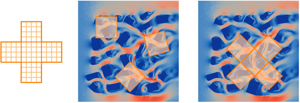
FIGURE 1. Left: the star-shaped grid; centre: random placement of central subdomain of the grid (for obtaining data to train CAEs); right: random placement of the star-shaped grid (for obtaining data to train the predictive adversarial network).
2.2 Dimensionality Reduction
Having been shown to compress data well for advection-dominated flows, we choose the convolutional autoencoder to reduce the dimension of the problem and find the low-dimensional subspace in which the HFM will be approximated. The CAE has been widely applied to reduced-order models in recent years and more details about this type of network along with schematic diagrams can be found in Gonzalez and Balajewicz [42], Xu and Duraisamy [43], Wu et al. [44], Nikolopoulos et al. [45]. In a nutshell, the CAE is a type of feed-forward neural network with convolutional layers that attempts to learn the identity map [46]. When used for compression, the CAE has a central ‘bottleneck’ layer which has fewer neurons than the input and output layers. The values of the neurons in this central layer are known as latent variables or reduced variables. The outer layers of the network consist of convolutional layers (which detect patterns or features in the flow fields) and pooling layers (which reduce the dimensions of the data), and at the centre of the network are fully connected layers. The autoencoder can be split into an encoder, which maps the input to the latent variables (compressing the data) and a decoder which maps the latent variables to the output (reconstructing the data). If
where ug,C represents the velocity field that has been interpolated onto the central subdomain of structured grid g and is the input to the autoencoder, and
A second CAE was trained to compress the buildings field, using data from Ng snapshots. The reduced variables associated with the buildings field can be written as
where bg,C is the buildings field of subdomain s of grid g. Figure 1B shows three such subdomains, randomly located and orientated within the domain, and superposed on the velocity field of the test case at a particular time. Although we could have used data from all the subdomains to train the autoencoders, we found this not to be necessary and only used data from the central subdomains. We do, however, obtain the reduced variables for any subdomain (N, E, W, S or C) with the trained encoder.
2.3 Prediction in Time
In this work, we follow [3] by modifying the adversarial autoencoder so that it can predict in time, and refer to it as a “Predictive Adversarial Network” (PAN). The adversarial autoencoder [24] uses an adversarial strategy to force the autoencoder’s latent space to follow a prior distribution (Pprior) whilst the output aims to replicate the input as closely as possible. Thus, in addition to the encoder-decoder networks of a standard autoencoder, the adversarial autoencoder has a discriminator (the adversarial network) which is connected to the central layer of the encoder-decoder. The discriminator is trained to distinguish between samples from the prior distribution (true samples) and samples from latent space (fake samples). The modifications made to the adversarial autoencoder include: the inputs and outputs no longer have the same dimension (as is required for autoencoders that learn the identity map); the width of the layers does not fall below the width of the output layer (preventing additional compression to that already performed in the dimensionality reduction stage); and the loss function no longer minimises the difference between its input and output, rather the output and the desired output. A schematic diagram of the PAN can be seen in Figure 2, where
where
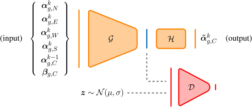
FIGURE 2. The predictive adversarial network. The generator is represented by
For the prediction network, data from all five subdomains is used for training and inference, as shown in Figure 3. The star-shaped grid is used, as, when predicting in time, it is beneficial to have information from neighbouring regions. The input to the network consists of the reduced variables associated with the four neighbouring subdomains at the future time level (tk) (see Figure 3(left)); the reduced variables associated with the central grid at the current time (tk−1) (see Figure 3(left)); and the reduced variables associated with the central subdomain that describe the buildings. The output of the network is the reduced variables associated with the central subdomain at the future time level (see Figure 3(right)). If the predictive adversarial network is represented by f, this can be written as
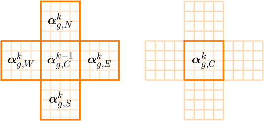
FIGURE 3. Left: reduced variables associated with the five subdomains (N, E, W, S, and C) of the star-shaped grid at future (k) and current (k − 1) time levels, which, along with the reduced variables of the buildings (βg,C), form the input to the neural network; right: the reduced variables of the central grid at the future time level which form the output of the neural network.
2.4 Prediction for Unseen Scenarios
In order to increase the generalisation properties of the reduced-order model, in addition to using a sub-sampling technique to obtain the snapshots (as described in Section 2.1, we pose each new scenario within a domain decomposition framework.
2.4.1 Combining Subdomains to Model an Unseen Scenario
Having trained neural networks to be able to predict flows within a subdomain given the flows in neighbouring subdomains and the layout of the buildings, a new (and therefore unseen) domain can be constructed from a non-overlapping union of these subdomains. Initial conditions for both the velocity and buildings fields are required, which are then encoded by the convolutional autoencoders. This provides a starting point from which to evolve the reduced variables in time. At a given time level, a prediction is made for the subdomains one-by-one (see Figure 4), with the variables being updated as and when the solutions are available in the manner of Gauss-Seidel iteration. An iteration-by-subdomain approach is used until convergence of the global solution is reached at that time level, and the process continues to find the solution at the next time level. In this manner, the solution of the NIROM is marched forward in time from an initial condition. Figure 4 is a schematic diagram that shows how domain decomposition can be used to form an array of subdomains, and how the PAN is used with iteration-by-subdomain to solve for the global solution. This approach for prediction of flows for an unseen arrangement of buildings is summarised in Algorithm 1.
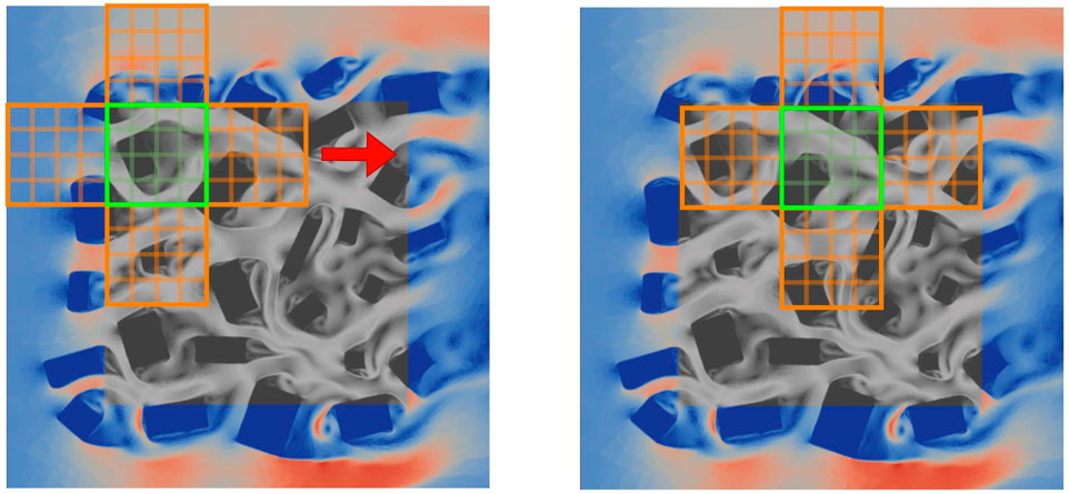
FIGURE 4. Greyscale regions indicate the area where we seek a solution. The coloured regions show the magnitude of the velocity of the imposed boundary conditions. Left: Using the latest solutions of the four neighbouring subdomains (indicated in orange), and the previous solution in the central subdomain (shown in green) and the buildings fields in the central subdomain, a prediction is made for the central subdomain. Right: move to the next set of five subdomains and predict for the next central subdomain.
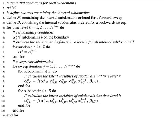
Algorithm 1. An algorithm for finding the solution for the reduced variables in a subdomain and sweeping over all the subdomains to obtain a converged solution over the whole domain. The algorithm marches forward in time from the initial condition to time level Ntime.
3 Results
The methods described previously are now tested on flow past buildings modelled in 2D. Assuming an incompressible viscous fluid, the conservation of mass and the Navier-Stokes equations can be written as
where t represents time, v represents velocity, p represents pressure, μ is the dynamic viscosity, ρ is the density and σ is an absorption term that is zero outside the buildings and 106 inside the buildings. The boundary conditions that we use in conjunction with Equations 6 and 7 are defined as follows. At the inlet we specify the normal velocity component which we set to unity. The tangential components at the inlet boundary on the left of the domains (see, for example, Figure 6) are set to zero. We also set a zero normal velocity boundary condition to the top and bottom boundaries of this domain along with a zero shear stress condition. At the outlet we set the normal and shear stress components to zero which effectively sets the pressure to near zero at the outlet. Equations 6 and 7 together with the boundary conditions are discretised using a finite element representation for velocity and a control volume representation of pressure [47] combined in a P1DG-P1CV element [48,49]. An unstructured mesh is used which adapts through time, and an adaptive time step is also used. For more details of how the governing equations are discretised and solved, see Obeysekara et al. [48].
For ease of setting up this test case, we represent the areas occupied by buildings as a sink in the velocity field (through an absorption coefficient which acts on the velocity field, which can be seen in the term involving σv in Eq. 7). By using adaptive meshes (adapting to σ and the velocity field), we obtain a sharp boundary between the buildings and the outside air flow, although this would be sharper if the building had been modelled explicitly. In any case, we believe that the CFD results are a good enough representation of flow past buildings to be used in this proof-of-concept paper.
The numerical solutions were found for two domains, one measuring 6 by 6 and the other measuring 9 by 9. These domains were populated with randomly located and orientated buildings. The lengths of both edges of each building were chosen randomly from the interval [0.1, 0.4] and a minimum gap of 0.075 was enforced between the buildings. A gap between the domain boundaries and the buildings was maintained. In practice the number of buildings for the 6 by 6 and 9 by 9 case is about 150 and 340 respectively.
A Reynolds number of 300 was used in both the simulations, and was based on the unity inlet velocity and minimum building edge length. The actual time step size was controlled by the Courant number, chosen to be 0.5, and the solutions were saved every 0.008 time units, giving the NIROM a time step size of 0.008. For a regular array of 17 square cylinders, Shams-ul Islam et al. [50] observed chaotic flows for Reynolds numbers greater than 125. In our case, we believe that Re = 300 is more than sufficient for the flow to be chaotic and therefore to present an interesting modelling challenge.
3.1 Dimensionality Reduction
The solutions from the 6 by 6 test case were interpolated onto central subdomains of size 0.5 by 0.5 for every time level. 95,000 snapshots were created in total for the velocity CAE (by selecting 95,000 randomly located and orientated grids, at a randomly selected time levels): 76,000 snapshots were used for training data and the remaining 19,000 snapshots were used as validation data. For the buildings field, a similar procedure was used to generate 95,000 snapshots. However, as the buildings do not change in time, there was no random sampling in time. After optimisation of both networks simultaneously, the chosen hyperparameter values are shown in Table 1 and the architectures can be found in Table 2. Figure 5 shows the velocity and buildings fields from the HFM (unseen example) and the reconstruction from the autoencoders for one subdomain. The velocity components are very well reconstructed and the buildings field is captured well. The pointwise error of the latter is confined to an extremely small region around the edge of the buildings.
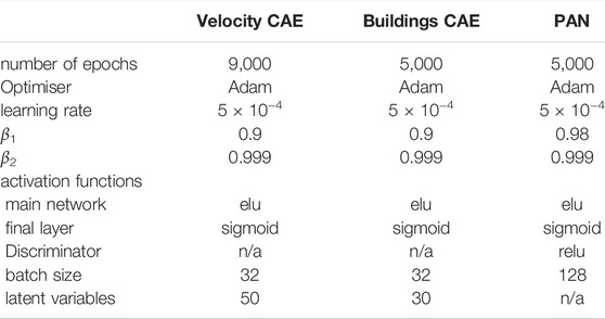
TABLE 1. Hyperparameter values used in the neural networks. Associated with the optimiser, β1 and β2 are the exponential decay rate for the first moment estimates and the exponential decay rate for the exponentially weighted infinity norm respectively.
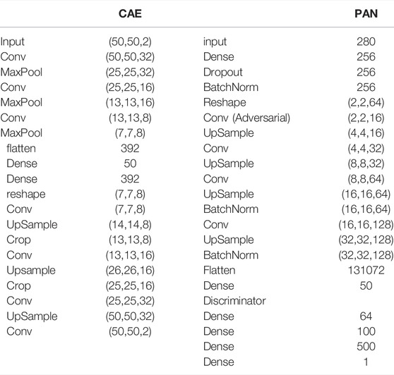
TABLE 2. Left: architecture of the CAE for the velocity field. (The architecture of the CAE for the buildings field is similar, but with an input of (50,50,1) and a central dense layer of 30 neurons.) Right: architecture of the PAN.
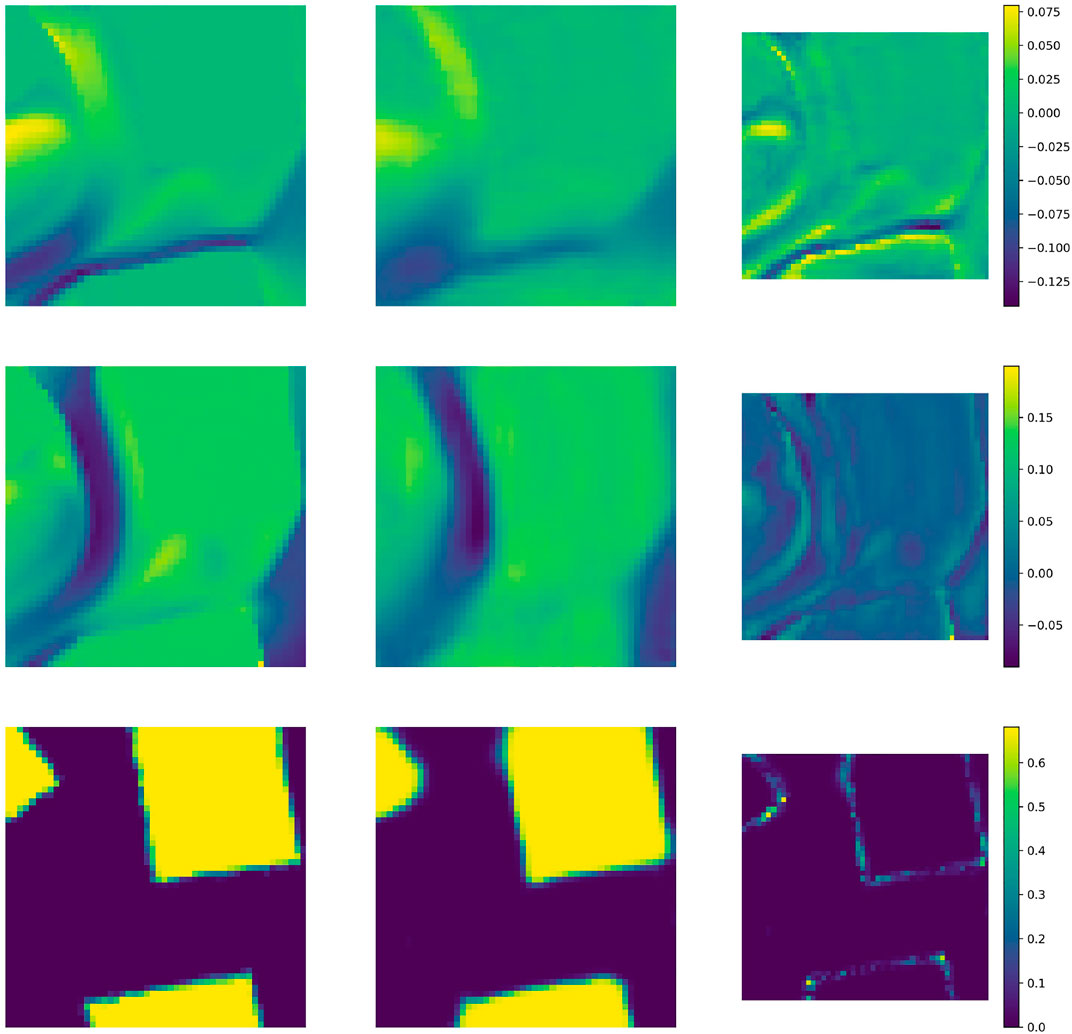
FIGURE 5. Plots to demonstrate the quality of the autoencoders. The (unseen) solutions associated with one subdomain are compressed and reconstructed. Left column: results from the HFM; central column: reconstruction from the CAE; right column: pointwise difference. Top row: x − component of velocity; middle row: y − component of velocity; bottom row: buildings field.
3.2 Prediction for the 6 by 6 Test Case
The solutions from the 6 by 6 test case were interpolated onto the star-shaped grids (see Figure 1), within which, each subdomain is of size 0.5 by 0.5 (one 12th of the domain size and thus 144 subdomains fit into the 6 by 6 domain). To form an input-output pair for training, two successive time levels were chosen at random (from time levels 50 to 349) and the velocity fields associated with both time levels were interpolated onto the grid in order to have all the variables required by the PAN, see Eq. 5. The buildings field was interpolated onto the central subdomain of the grid. 75,000 snapshots were created in total for the PAN: 50,000 input-output pairs were used for training data and the remaining 25,000 input-output pairs were used as validation data. Hyperparameter optimisation was performed, revealing the optimal values for the PAN which are shown in Table 1, and the architectures in Table 2.
Once trained, the method is tested by predicting in time. An initial condition is used, based on the HFM results at time level 50, and the method described in Algorithm 1 and the accompanying text is used to march forward from time level 50 up to time level 400. Figures 6 and 7 show the prediction of the adversarial network for two particular time levels beyond the training dataset but for the same buildings configuration as the training dataset. The ROM captures the velocity magnitudes well. It has managed to capture the areas where there are high velocities, in comparison to the HFM, although its resolution is reduced. Impressively, it is also able to capture many of the eddy structures that result from the interaction of the fluid with the buildings. Again we assume the truth is the HFM simulation when comparing the two images. This NIROM simulation would be expected, eventually, to deviate from the HFM as it is a chaotic flow and small velocity deviations will build up, potentially changing the flow structures significantly.
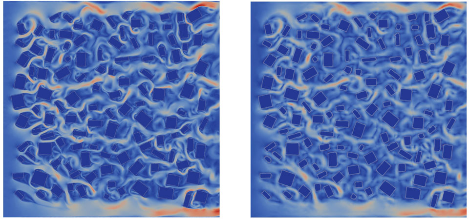
FIGURE 6. The velocity magnitude at the 350th time level from the HFM (left) and the predictive adversarial network (right).
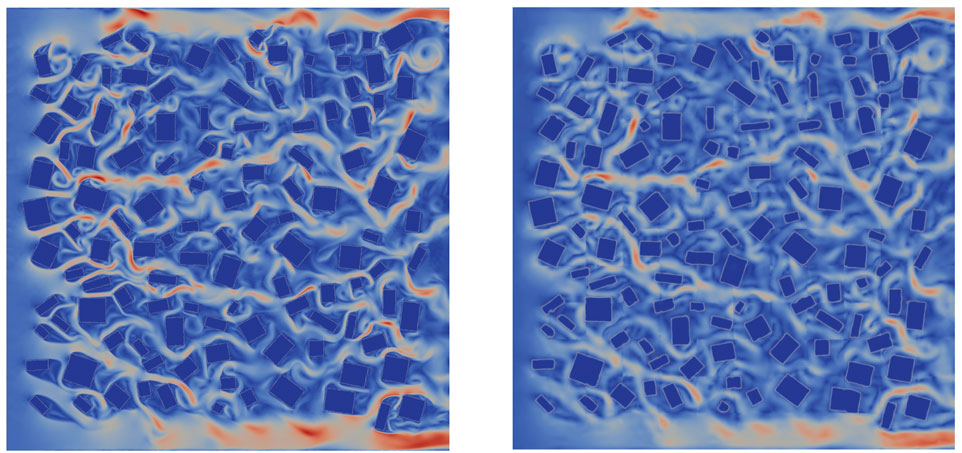
FIGURE 7. The velocity magnitude at the 400th time level from the HFM (left) and the predictive adversarial network (right).
In Figure 8 we plot all the nodes within the domain, with the nodes inside buildings appearing as blue and those outside the buildings as red. Thus we can see the position of the buildings and the density of the mesh at this instance in time, which corresponds to the results shown in Figure 6. We also show four points within the domain, in black, where we will plot the histograms, or probability density functions, of the x − and y − components of velocity, taken over time level 50 to time level 400. These histograms are shown in Figure 9 and the coordinates of the points are given in Table 3. We see a qualitative agreement in terms of the statistics of the fluctuations and the range of velocities between the HFM and the NIROM. The narrower the histograms, the smaller the magnitude of the fluctuations in the velocity components. Thus, generally speaking the NIROM tends to fluctuate less than the HFM, probably because it has a little less resolution than the HFM. It also (again because of reduced resolution) has less frequently occurring large values of the velocity. However, given the complexity of the flows, the NIROM does remarkably well, even though there are some histograms that do not compare quite so well, such as the x − component of the velocity at point 4.
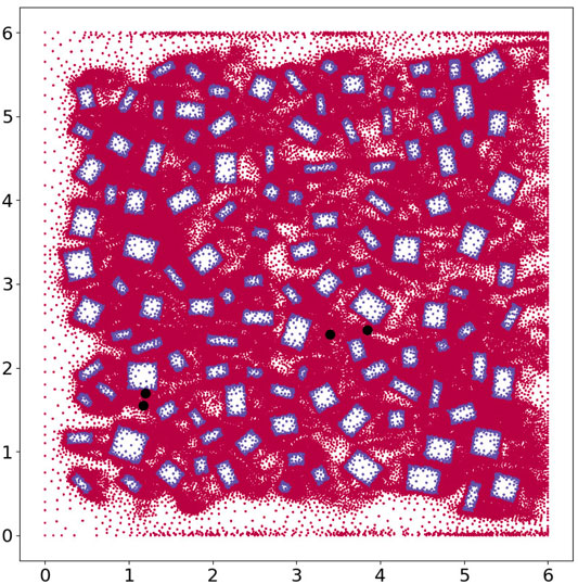
FIGURE 8. Here we plot all the nodes within the 6 by 6 domain. The nodes within the building appear as blue and those outside of the building as red. We also show four points within the domain, in black, where we plot the histograms, or probability density functions, of the x − and y − components of velocity.
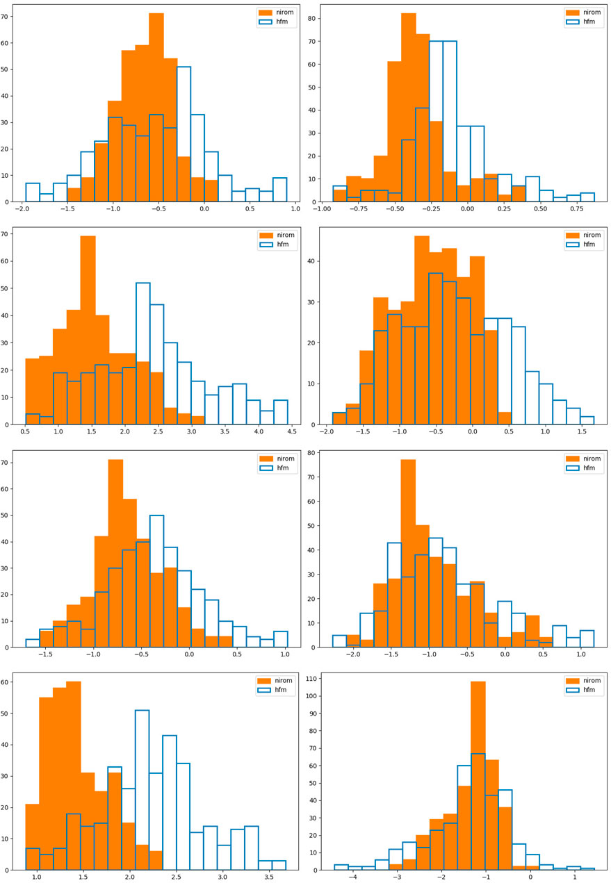
FIGURE 9. Here we show histograms for the 6 by 6 test case at points 1, 2, 3 and 4 (see Table 3) in rows from top to bottom respectively. The first column of graphs show the x − component of velocity and the second the y − component. We compare in these graphs the histograms (or probability density functions) of the velocity components of the HFM in blue, and NIROM in orange.
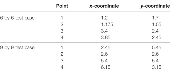
TABLE 3. The coordinates of the points at which the probability distributions are generated for both the 6 by 6 case and the 9 by 9 case.
3.3 Prediction for the Unseen 9 by 9 Test Case
Now an unseen configuration of buildings is used and the domain is increased from 6 by 6 to 9 by 9. The HFM is solved in order to have boundary conditions for the ROM. In the future, alternative methods to generate boundary conditions will be explored, including methods based on using the training data from the HFM [3], but also methods based on generative networks, which will ensure that the ROM is independent of the HFM in this regard. The initial condition for the NIROM is taken from time level 50 of the HFM. The domain is now split into 324 subdomains (of size 0.5 by 0.5). The predictive adversarial network is used to generate a solution for each internal subdomain (i.e., each subdomain that does not share an edge with the boundary). All internal subdomains are swept through until the global solution converges. Time-marching is applied to solve from the initial condition at time level 50 to time level 250, as outlined in Algorithm 1. Within each time step, the number of iterations needed for convergence is approximately 20, about 4 more than for the previous 6 by 6 problem. Convergence is assumed when the difference between latent variables associated with compressed velocity (outputs of the PAN in each of the 324 subdomains) is less than e − 4 given that the magnitude of the latent variables is
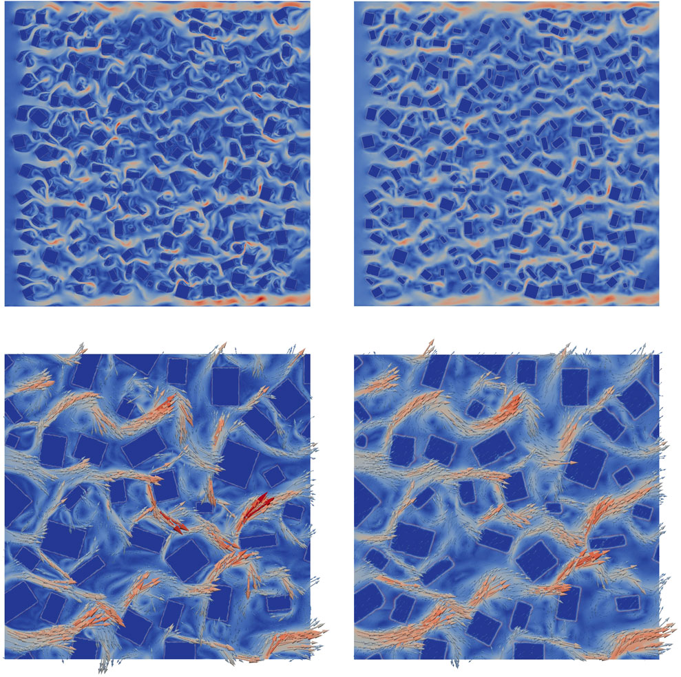
FIGURE 10. Velocity magnitude across the 9 by 9 domain at time level 250. Top left: HFM, and top right: prediction by the ROM. Bottom left and right: velocity vectors over a 3 by 3 region [1,4]×[4,7] of the 9 by 9 domain, for HFM and NIROM respectively.
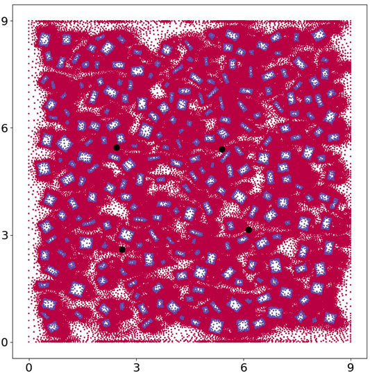
FIGURE 11. Here we plot all the nodes within the 9 by 9 domain. The nodes within the building appear as blue and those outside of the building as red. We also show four points within the domain, in black, where we plot the histograms, or probability density functions, of the x − and y − components of velocity.
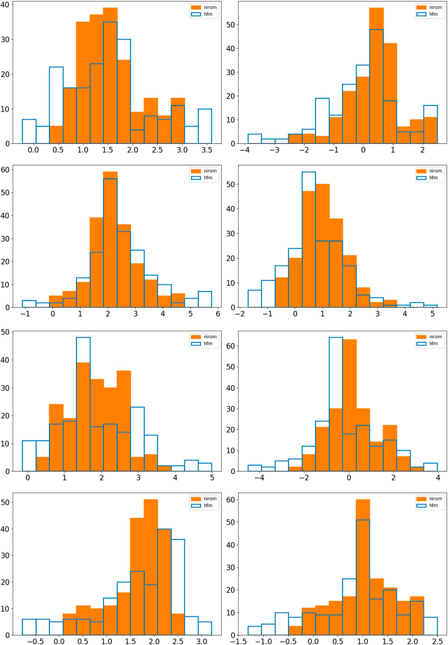
FIGURE 12. Here we show histograms for the 9 by 9 test case at points 1, 2, 3 and 4 (see Table 3) in rows from top to bottom respectively. The first column of graphs show the x − component of velocity and the second the y − component. We compare in these graphs the histograms (or probability density functions) of the velocity components of the HFM (not seen in training), blue, and the prediction from NIROM in orange.
4 Conclusions and Further Work
Here we have presented a data-driven or Machine Learning (ML) based non-intrusive reduced-order model (NIROM) which is capable of making predictions for a significantly larger domain than the one used to generate the snapshots or training data. This is a unique development and one which we hope paves the way to develop ML-based NIROMs that can make good predictions for unseen scenarios. Ultimately these methods could complement Computational Fluid Dynamics (CFD) codes when solving flow fields in urban environments as well as other CFD applications. This development relies on the combination of a novel way of sampling the training data [which can free the reduced-order model from the restriction of the domain of the high-fidelity model (HFM)] and a domain decomposition approach (which decomposes unseen geometries in a manner consistent with the sub-sampling approach).
The main conclusions are that: (1) one can predict (with the NIROM) the chaotic transient flows within the 2D problems, although sometimes the resolution is reduced in comparison to the CFD simulations; (2) the adversarial layer of the prediction algorithm is important in order to form stable solutions that remain within the distribution of the training data; (3) a convolutional autoencoder is able to compress the velocity and buildings fields to a high degree of accuracy; and (4) the approach was applied to make predictions for a domain of over twice the area and over twice the number of buildings as in the HFM used to generate the training data.
Future work will involve: (1) extending the problem domains to 3D and using more realistic building profiles; (2) generating boundary conditions with a generative network rather than using the CFD code, resulting in a method fully independent of the high-fidelity model; (3) using the residuals of the differential equations within the training procedure (Physics-Informed methods, for example, see [51]) and forcing the equation residuals to zero within the prediction step by using a method similar to the Residual DEIM approach [52].
Data Availability Statement
The raw data supporting the conclusions of this article will be made available by the authors, without undue reservation.
Author Contributions
CH, CP, PS, and IN contributed to conception and design of the study. XL, HG, ZW, CH, and CP worked on the software. CH, XL, HG, and CP worked on the methodology. CH, XL, HG, and CP worked on the first draft of the manuscript. All authors contributed to manuscript revision, read, and approved the submitted version.
Funding
The authors would like to acknowledge the following EPSRC grants: RELIANT, Risk EvaLuatIon fAst iNtelligent Tool for COVID19 (EP/V036777/1); MAGIC, Managing Air for Green Inner Cities (EP/N010221/1); MUFFINS, MUltiphase Flow-induced Fluid-flexible structure InteractioN in Subsea applications (EP/P033180/1); the PREMIERE programme grant (EP/T000414/1); and INHALE, Health assessment across biological length scales (EP/T003189/1).
Conflict of Interest
The authors declare that the research was conducted in the absence of any commercial or financial relationships that could be construed as a potential conflict of interest.
Publisher’s Note
All claims expressed in this article are solely those of the authors and do not necessarily represent those of their affiliated organizations, or those of the publisher, the editors and the reviewers. Any product that may be evaluated in this article, or claim that may be made by its manufacturer, is not guaranteed or endorsed by the publisher.
Acknowledgments
We are grateful to Imperial College for use of their UKRI Open Access Block Grant, which has funded publication of this work. We would also like to thank the reviewers for their comments and suggestions, which have improved the paper.
References
1.W Schilders, H van der Vorst, and J Rommes, editors. Model Order Reduction: Theory, Research Aspects and Applications. Springer (2008). vol. 13 of The European Consortium for Mathematics in Industry.
2. Benner P, Gugercin S, Willcox K. A Survey of Projection-Based Model Reduction Methods for Parametric Dynamical Systems. SIAM Rev (2015) 57:483–531. doi:10.1137/130932715
3. Heaney CE, Wolffs Z, Tómasson JA, Kahouadji L, Salinas P, Nicolle A, et al. An AI-Based Non-intrusive Reduced-Order Model for Extended Domains Applied to Multiphase Flow in Pipes. Phys Fluids (2022) 34:055111. doi:10.1063/5.0088070
4. Brunton SL, Noack BR, Koumoutsakos P. Machine Learning for Fluid Mechanics. Annu Rev Fluid Mech (2020) 52:477–508. doi:10.1146/annurev-fluid-010719-060214
5. Buchan AG, Pain CC, Fang F, Navon IM. A POD Reduced-Order Model for Eigenvalue Problems with Application to Reactor Physics. Int J Numer Meth Engng (2013) 95:1011–32. doi:10.1002/nme.4533
6. Fang F, Zhang T, Pavlidis D, Pain CC, Buchan AG, Navon IM. Reduced Order Modelling of an Unstructured Mesh Air Pollution Model and Application in 2D/3D Urban Street Canyons. Atmos Environ (2014) 96:96–106. doi:10.1016/j.atmosenv.2014.07.021
7. Ballarin F, Rozza G. POD-galerkin Monolithic Reduced Order Models for Parametrized Fluid-Structure Interaction Problems. Int J Numer Meth Fluids (2016) 82:1010–34. doi:10.1002/fld.4252
8. Fukami K, Murata T, Zhang K, Fukagata K. Sparse Identification of Nonlinear Dynamics with Low-Dimensionalized Flow Representations. J Fluid Mech (2021) 926:A10. doi:10.1017/jfm.2021.697
9. Kadeethum T, Ballarin F, Choi Y, O’Malley D, Yoon H, Bouklas N. Non-intrusive Reduced Order Modeling of Natural Convection in Porous media Using Convolutional Autoencoders: Comparison with Linear Subspace Techniques. Adv Water Resour (2022) 160:104098. doi:10.1016/j.advwatres.2021.104098
10. Maulik R, Lusch B, Balaprakash P. Reduced-order Modeling of Advection-Dominated Systems with Recurrent Neural Networks and Convolutional Autoencoders. Phys Fluids (2021) 33:037106. doi:10.1063/5.0039986
11. Audouze C, De Vuyst F, Nair PB. Nonintrusive Reduced-Order Modeling of Parametrized Time-dependent Partial Differential Equations. Numer Methods Partial Differential Eq (2013) 29:1587–628. doi:10.1002/num.21768
12. Bui-Thanh T, Damodaran M, Willcox K. Proper Orthogonal Decomposition Extensions for Parametric Applications in Compressible Aerodynamics. In: 21st AIAA Applied Aerodynamics Conference (2003). Florida: AIAA. doi:10.2514/6.2003-4213
13. Guénot M, Lepot I, Sainvitu C, Goblet J, Filomeno Coelho R. Adaptive Sampling Strategies for Non‐intrusive POD‐based Surrogates. Eng Computations (2013) 30:521–47. doi:10.1108/02644401311329352
14. Hesthaven JS, Ubbiali S. Non-intrusive Reduced Order Modeling of Nonlinear Problems Using Neural Networks. J Comput Phys (2018) 363:55–78. doi:10.1016/j.jcp.2018.02.037
15. Wang Z, Xiao D, Fang F, Govindan R, Pain CC, Guo Y-K. Model Identification of Reduced Order Fluid Dynamics Systems Using Deep Learning. Int J Numer Methods Fluids (2017) 86:255–68. doi:10.1002/fld.4416
16. Wiewel S, Becher M, Thuerey N. Latent Space Physics: Towards Learning the Temporal Evolution of Fluid Flow. Comput Graphics Forum (2019) 38:71–82. doi:10.1111/cgf.13620
17. Maulik R, Botsas T, Ramachandra N, Mason LR, Pan I. Latent-space Time Evolution of Non-intrusive Reduced-Order Models Using Gaussian Process Emulation. Physica D: Nonlinear Phenomena (2021) 416:132797. doi:10.1016/j.physd.2020.132797
18. Ahmed SE, San O, Rasheed A, Iliescu T. Nonlinear Proper Orthogonal Decomposition for Convection-Dominated Flows. Phys Fluids (2021) 33:121702. doi:10.1063/5.0074310
19. Fresca S, Manzoni A. POD-DL-ROM: Enhancing Deep Learning-Based Reduced Order Models for Nonlinear Parametrized PDEs by Proper Orthogonal Decomposition. Comput Methods Appl Mech Eng (2022) 388:114181. doi:10.1016/j.cma.2021.114181
20. Maulik R, Lusch B, Balaprakash P. Non-autoregressive Time-Series Methods for Stable Parametric Reduced-Order Models. Phys Fluids (2020) 32:087115. doi:10.1063/5.0019884
21. Quilodrán-Casas C, Arcucci R, Mottet L, Guo Y-K, Pain CC. Adversarial Autoencoders and Adversarial LSTM for Improved Forecasts of Urban Air Pollution Simulations (2021). arXiv. doi:10.48550/arXiv.2104.06297
22. Quilodrán-Casas C, Arcucci R, Pain CC, Guo Y-K. Adversarially Trained LSTMs on Reduced Order Models of Urban Air Pollution Simulations (2021). arXiv. doi:10.48550/arXiv.2101.01568
23. Goodfellow IJ, Pouget-Abadie J, Mirza M, Xu B, Warde-Farley D, Ozair S, et al. Generative Adversarial Networks (2014). arXiv. doi:10.48550/arXiv.1406.2661
24. Makhzani A, Shlens J, Jaitly N, Goodfellow I, Frey B. Adversarial Autoencoders (2015). arXiv. doi:10.48550/arXiv.1511.05644
25. Cheng M, Fang F, Pain CC, Navon IM. An Advanced Hybrid Deep Adversarial Autoencoder for Parameterized Nonlinear Fluid Flow Modelling. Comput Methods Appl Mech Eng (2020) 372:113375. doi:10.1016/j.cma.2020.113375
26. Silva VLS, Heaney CE, Pain CC. Data Assimilation Predictive GAN (DA-PredGAN): Applied to Determine the Spread of COVID-19 (2021). arXiv. doi:10.48550/arXiv.2105.07729
27. Sanchez-Gonzalez A, Godwin J, Pfaff T, Ying R, Leskovec J, Battaglia PW. Learning to Simulate Complex Physics with Graph Networks. In: A Singh, editors. Proceedings of the 37th International Conference on Machine Learning (PMLR) (2020). jmlr.org
28. Baiges J, Codina R, Idelsohn S. A Domain Decomposition Strategy for Reduced Order Models. Application to the Incompressible Navier-Stokes Equations. Comput Methods Appl Mech Eng (2013) 267:23–42. doi:10.1016/j.cma.2013.08.001
29. Xiao D, Fang F, Heaney CE, Navon IM, Pain CC. A Domain Decomposition Method for the Non-intrusive Reduced Order Modelling of Fluid Flow. Comput Methods Appl Mech Eng (2019) 354:307–30. doi:10.1016/j.cma.2019.05.039
30. Xiao D, Heaney CE, Fang F, Mottet L, Hu R, Bistrian DA, et al. A Domain Decomposition Non-intrusive Reduced Order Model for Turbulent Flows. Comput Fluids (2019) 182:15–27. doi:10.1016/j.compfluid.2019.02.012
31. Yang LM, Grooms I. Machine Learning Techniques to Construct Patched Analog Ensembles for Data Assimilation. J Comput Phys (2021) 443:110532. doi:10.1016/j.jcp.2021.110532
32. Schmid PJ. Dynamic Mode Decomposition of Numerical and Experimental Data. J Fluid Mech (2010) 656:5–28. doi:10.1017/S0022112010001217
33. Brunton SL, Proctor JL, Kutz JN. Discovering Governing Equations from Data by Sparse Identification of Nonlinear Dynamical Systems. Proc Natl Acad Sci U.S.A (2016) 113:3932–7. doi:10.1073/pnas.1517384113
34. Brunton SL, Kutz JN. Methods for Data-Driven Multiscale Model Discovery for Materials. J Phys Mater (2019) 2:044002. doi:10.1088/2515-7639/ab291e
35. Bistrian DA, Navon IM. An Improved Algorithm for the Shallow Water Equations Model Reduction: Dynamic Mode Decomposition vs POD. Int J Numer Meth Fluids (2015) 78:552–80. doi:10.1002/fld.4029
36. Carlberg KT, Jameson A, Kochenderfer MJ, Morton J, Peng L, Witherden FD. Recovering Missing CFD Data for High-Order Discretizations Using Deep Neural Networks and Dynamics Learning. J Comput Phys (2019) 395:105–24. doi:10.1016/j.jcp.2019.05.041
37. Eivazi H, Veisi H, Naderi MH, Esfahanian V. Deep Neural Networks for Nonlinear Model Order Reduction of Unsteady Flows. Phys Fluids (2020) 32:105104. doi:10.1063/5.0020526
38. Vlachas PR, Arampatzis G, Uhler C, Koumoutsakos P. Multiscale Simulations of Complex Systems by Learning Their Effective Dynamics. Nat Machine Intelligence (2022) 4:359–66. doi:10.1038/s42256-022-00464-w
39. Hasegawa K, Fukami K, Murata T, Fukagata K. Machine-learning-based Reduced-Order Modeling for Unsteady Flows Around bluff Bodies of Various Shapes. Theor Comput Fluid Dyn (2020) 34:367–83. doi:10.1007/s00162-020-00528-w
40. Gastaldi L. A Domain Decomposition Method Associated with the Streamline Diffusion FEM for Linear Hyperbolic Systems. Appl Numer Maths (1992) 10:357–80. doi:10.1016/0168-9274(92)90057-K
41. Pain C, Umpleby A, de Oliveira C, Goddard A. Tetrahedral Mesh Optimisation and Adaptivity for Steady-State and Transient Finite Element Calculations. Comput Methods Appl Mech Eng (2001) 190:3771–96. doi:10.1016/S0045-7825(00)00294-2
42. Gonzalez FJ, Balajewicz M. Deep Convolutional Recurrent Autoencoders for Learning Low-Dimensional Feature Dynamics of Fluid Systems (2018). arXiv. doi:10.48550/arXiv.1808.01346
43. Xu J, Duraisamy K. Multi-level Convolutional Autoencoder Networks for Parametric Prediction of Spatio-Temporal Dynamics. Comput Methods Appl Mech Eng (2020) 372:113379. doi:10.1016/j.cma.2020.113379
44. Wu P, Gong S, Pan K, Qiu F, Feng W, Pain CC. Reduced Order Model Using Convolutional Auto-Encoder with Self-Attention. Phys Fluids (2021) 33:077107. doi:10.1063/5.0051155
45. Nikolopoulos S, Kalogeris I, Papadopoulos V. Non-intrusive Surrogate Modeling for Parametrized Time-dependent PDEs Using Convolutional Autoencoders (2021). arXiv. doi:10.48550/arXiv.2101.05555
46. Makkie M, Huang H, Zhao Y, Vasilakos AV, Liu T. Fast and Scalable Distributed Deep Convolutional Autoencoder for fMRI Big Data Analytics. Neurocomputing (2019) 325:20–30. doi:10.1016/j.neucom.2018.09.066
47. Salinas P, Pavlidis D, Xie Z, Jacquemyn C, Melnikova Y, Jackson MD, et al. Improving the Robustness of the Control Volume Finite Element Method with Application to Multiphase Porous media Flow. Int J Numer Methods Fluids (2017) 85:235–46. doi:10.1002/fld.4381
48. Obeysekara A, Salinas P, Heaney CE, Kahouadji L, Via-Estrem L, Xiang J, et al. Prediction of Multiphase Flows with Sharp Interfaces Using Anisotropic Mesh Optimisation. Adv Eng Softw (2021) 160:103044. doi:10.1016/j.advengsoft.2021.103044
49. Via-Estrem L, Salinas P, Xie Z, Xiang J, Latham J-P, Douglas S, et al. Robust Control Volume Finite Element Methods for Numerical Wave Tanks Using Extreme Adaptive Anisotropic Meshes. Int J Numer Methods Fluids (2020) 92:1707–22. doi:10.1002/fld.4845
50. Shams-ul Islam S, Nazeer G, Ying ZC. Numerical Investigation of Flow Past 17-cylinder Array of Square Cylinders. AIP Adv (2018) 8:065004. doi:10.1063/1.5022360
51. Chen W, Wang Q, Hesthaven JS, Zhang C. Physics-informed Machine Learning for Reduced-Order Modeling of Nonlinear Problems. J Comput Phys (2021) 446:110666. doi:10.1016/j.jcp.2021.110666
Keywords: data-driven reduced-order modelling, non-intrusive reduced-order modelling, adversarial neural network, autoencoder, urban flows, machine learning, generalisation, inference
Citation: Heaney CE, Liu X, Go H, Wolffs Z, Salinas P, Navon IM and Pain CC (2022) Extending the Capabilities of Data-Driven Reduced-Order Models to Make Predictions for Unseen Scenarios: Applied to Flow Around Buildings. Front. Phys. 10:910381. doi: 10.3389/fphy.2022.910381
Received: 01 April 2022; Accepted: 30 May 2022;
Published: 04 July 2022.
Edited by:
Traian Iliescu, Virginia Tech, United StatesReviewed by:
Kai Fukami, University of California, United StatesPing-Hsuan Tsai, University of Illinois at Urbana-Champaign, United States
Copyright © 2022 Heaney, Liu, Go, Wolffs, Salinas, Navon and Pain. This is an open-access article distributed under the terms of the Creative Commons Attribution License (CC BY). The use, distribution or reproduction in other forums is permitted, provided the original author(s) and the copyright owner(s) are credited and that the original publication in this journal is cited, in accordance with accepted academic practice. No use, distribution or reproduction is permitted which does not comply with these terms.
*Correspondence: Claire E. Heaney, Yy5oZWFuZXlAaW1wZXJpYWwuYWMudWs=
†These authors have contributed equally to this work
 Claire E. Heaney
 Xiangqi Liu1†
 Hanna Go
 Zef Wolffs
 Ionel M. Navon