Adulteration detection in minced beef using low-cost color imaging system coupled with deep neural network

Major processed meat products, including minced beef, are one of the favorite ingredients of most people because they are high in protein, vitamins, and minerals. The high demand and high prices make processed meat products vulnerable to adulteration. In addition, eliminating morphological attributes makes the authenticity of minced beef challenging to identify with the naked eye. This paper aims to describe the feasibility study of adulteration detection in minced beef using a low-cost imaging system coupled with a deep neural network. The proposed method was expected to be able to detect minced beef adulteration. There were 500 captured images of minced beef samples. Then, there were 24 color and textural features retrieved from the image. The samples were then labeled and evaluated. A deep neural network (DNN) was developed and investigated to support classification. The proposed DNN was also compared to six machine learning algorithms in the form of accuracy, precision, and sensitivity of classification. The feature importance analysis was also performed to obtain the most impacted features to classification results. The DNN model classification accuracy was 98.00% without feature selection and 99.33% with feature selection. The proposed DNN has the best performance with individual accuracy of up to 99.33%, a precision of up to 98.68%, and a sensitivity of up to 98.67%. This work shows the enormous potential application of a low-cost imaging system coupled with DNN to rapidly detect adulterants in minced beef with high performance.

Introduction

Minced beef, an essential ingredient in many popular foods such as meatballs, hamburgers, sausages, and patties, is widely consumed worldwide (Song et al., 2021). It is a popular food for most people and a great source of protein since it is packed with essential vitamins, minerals, and amino acids (Geiker et al., 2021). It is also easy to produce and handle, thus, making it a top choice for consumers (Song et al., 2021). Minced beef is vulnerable to adulteration due to the strong demand for minced beef products and an unfairly market system (Kumar and Chandrakant Karne, 2017; Rady and Adedeji, 2018; Zheng et al., 2019). Apparently, minced beef differs from raw beef. Minced beef loses the morphological characteristics of ground beef, making it challenging to identify adulterated minced beef depending on its color and textural properties (Fengou et al., 2021).

Minced beef adulteration is a significant concern for the food industry, negatively impacting brands, producers, and manufacturers. Adulteration is often done for economic reasons, making it possible to increase profits by lowering production costs by substituting cheap meat or offal for beef (Weng et al., 2020). The consequences are not only limited to consumer economic loss. But, they may have an impact on consumer health and lead to the consumption of unwanted meat products for religious or cultural reasons (Feng et al., 2018; Wahyuni et al., 2019). Since the 2013 horse meat scandal broke out, the adulteration of meat and meat products has attracted attention on a worldwide scale (Premanandh, 2013).

Accurate detection of minced beef adulteration will contribute to food protection throughout the supply chain. Currently, analytical techniques are based on protein and DNA analysis (Ballin, 2010; Erwanto et al., 2012). The European Parliament Resolution of January 14, 2014, states that DNA testing is a common practice for identifying meat from certain animal species and preventing adulteration (European Parliament, 2014). The standard method has high accuracy and resolution in identifying various adulterants in processed beef meat. However, this method has several disadvantages, including long-duration tests, high-cost instruments, and highly skilled workers' requirements (Beganović et al., 2019; Fengou et al., 2021). Therefore, this method is unsuitable for a rapid, non-laboratory environment, and fast customer authentication in the meat product supply chain.

Various methods have been investigated for the rapid detection of minced beef adulteration. It included spectroscopic (Silva et al., 2020; Weng et al., 2020) and hyperspectral imaging (HSI) techniques (Reis et al., 2018; Al-Sarayreh et al., 2020; Kamruzzaman, 2021). The advantages of spectroscopic methods are that it is non-destructive, fast, simple, and straightforward (Weng et al., 2020). However, the spectroscopic technique is a single-point measurement, which only produces information in the form of a spectrum. Spectral information does not fully represent adulteration due to the heterogeneous nature of minced beef that relies on spatial information obtained only through the imaging system. Thus, multispectral and hyperspectral imaging were investigated simultaneously. They could solve this spatial information issue because they could provide spectral and spatial information. However, both are expensive to implement on a rapid scale, while multispectral imaging systems (MSI) are limited by wavelength resolution (Roberts et al., 2018). The computational complexity is also challenged, especially in the hyperspectral data analysis (Reis et al., 2018).

Color imaging has been used to identify defects in some agricultural food products, such as fruits, vegetables, and meats. The use of color imaging on beef quality is often used to identify the quality through several parameters, such as color (Asmara et al., 2018), intramuscular fat (Du et al., 2008), and lean beef content (Hwang et al., 1997). Color imaging is also used to characterize and classify types of meats (Swartidyana et al., 2022). In 2021, Rady et al. showed the potential use of color vision using to detect minced beef adulteration. The results of these studies are pretty promising, with an accuracy of 41.0–89.7% in several adulteration schemes (Rady et al., 2021). They applied Linear Discriminant Analysis (LDA) coupled with ensemble methodology to enhance the classifier's performance. LDA is a simple, fast, and portable algorithm. However, it requires a typical distribution assumption on features or predictors. There are minimal studies on developing imaging systems for adulteration detection in meat products, including (Rady et al., 2021).

Imaging system coupled with neural network algorithms have various applications in the food quality and safety, including food classification, food calorie estimation, food supply chain monitoring, food quality detection, and food contamination detection (Sunil et al., 2021). Several studies showed that the dedicated system has great potential to be implemented in meat classification and quality detection. The neural network has been used to detect marbling in beef and pork (Liu et al., 2017), classify meat from different species (Al-Sarayreh et al., 2020), and classify different cut beef, based on the captured image (Sunil et al., 2021). However, no studies have been available on applying an imaging system coupled with a neural network for detecting adulteration in minced beef.

Color imaging with a consumer camera is very attractive because it offers affordability, convenience, portability, and simplicity for the adulteration detection of minced beef. However, a lot still needs to be explored further, especially in the image acquisition process, image system design, and image processing algorithms used to improve the accuracy of the detection and classification of adulterants. This study proposes an adulteration detection system based on a low-cost imaging system coupled with deep neural network (DNN) algorithms for minced beef.

Materials and methods

The proposed imaging system

Figure 1 represents the proposed imaging system's setup. The block diagram of the implemented imaging system is shown in Figure 2. The system consisted of a white light-emitting diode (LED) module as an illuminator. LED was located 15 cm vertically above the sample container. A CMOS color digital camera was used to capture the images. The LED module and camera were placed in a closed box with dimensions of 30 × 21.5 × 40 cm. The sample container was fixed and placed on a black surface. Each image was captured with the same system's setting, and the output image was stored in JPEG format with 1,920 × 1,080 pixels. The system was calibrated using an X-Rite color checker to ensure consistent image acquisition. The imaging system was connected to a personal computer via USB. All these works are implemented in the Python 3.8 as programming language using Google Colaboratory. The software implementation was done using a consumer grade personal computer with Intel Core i3-7020U CPU, 4 GB DDR4 RAM, and Intel^® HD Graphics 620 GPU card with 1 GB memory.

FIGURE 1

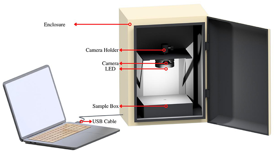
Figure 1. The proposed imaging system. The system consisted white LED and camera as the main component. Both were placed in a closed box. The sample container was fixed and placed on a black surface.

FIGURE 2

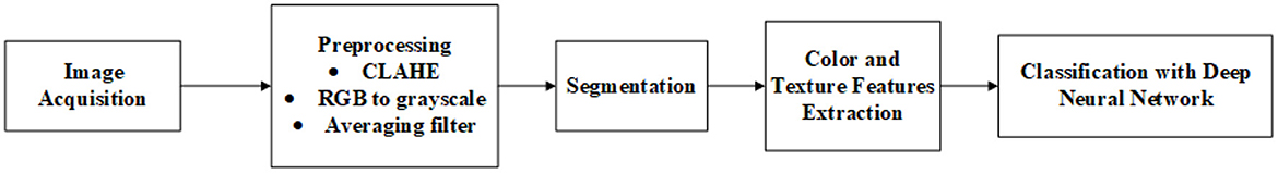
Figure 2. The workflow diagram of the implemented imaging system. First, image of samples was captured, labeled, and stored. Then, image preprocessing and segmentation was performed to determine the region of interest (ROI). Afterwards, color and textural features were extracted from the segmented image. Finally, deep neural network algorithm was implemented to perform classification.

Sample preparation

The raw meat samples used in this study were bought from the local market in Surabaya, Indonesia. The raw meat was transported to the laboratory within 1 h using an icebox container. The samples consisted of pure minced beef and adulterated minced beef, which contains five types of different adulterants, including lamb, pork, poultry, duck meat, and textured vegetable protein (TVP). The raw beef was minced using a laboratory-grade mincer and carefully washed and dried between preparations. Adulterated samples were prepared by manually mixing with gloved hands in the laboratory. The adulterated minced beef was made based on weight (w/w %). The adulterant level was 5–45% with a step of 5%, so there are nine samples for each adulterant. A total of 250 samples of pure minced beef and a total of 250 samples of adulterated minced beef (five different adulterants @500 samples) were prepared, each of 35 g (±5 g), for the investigation. Samples were placed on a suitable clean circular glass container with a diameter of ±3 cm.

Image acquisition

Each sample was placed in the translation stage according to the camera's field of view (FOV), as shown in Figure 1. Then, the captured image of the sample was acquired five times with a timer, and each captured image was labeled according to the class, the type of adulterants, and the adulteration levels. Then, the captured images were stored in a JPG format before being processed. A total of 2,500 images were acquired, and 500 were selected for further use as datasets. Figure 3 shows the tested samples' captured images and the number of samples.

FIGURE 3

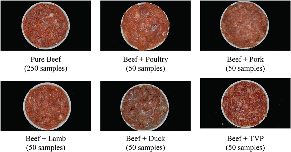
Figure 3. The examples of captured images of the pure and adulterated beef samples. The samples consisted of pure minced beef and adulterated minced beef (which contains five types of different adulterants, including lamb, pork, poultry, duck meat, and TVP). The number in parenthesis refers to the total of selected images for the referred adulterant.

Image preprocessing and segmentation

Figure 4 shows the illustration of pre-processing and segmentation process in this study. First, the image-enhancing algorithm was applied utilizing the concept of illumination reflection model based on Contrast Limited Adaptive Histogram Equalization (CLAHE). CLAHE has the advantage of overcoming contrast enhancement by assigning a limit value to the histogram (Pizer et al., 1987). After CLAHE was performed, the image was gray-scaled and smoothed by implementing a smoothing algorithm. Then, the process was continued into image thresholding using Otsu's thresholding and inverted binary thresholding to obtain a binary image. Otsu's thresholding processed image histograms, segmenting the objects by minimizing the variance in each class (Otsu, 1979). In Otsu's thresholding method, each possible threshold value is iterated over in order to determine the spread for the pixel levels on either side of the threshold, or the pixels that are either in the foreground or background. The goal of Otsu thresholding is to find the threshold value at which the total of foreground and background spreads is at its lowest. The weighted within class variances of these two classes are then minimized using the optimal threshold value that was calculated before (Liu and Yu, 2009). After thresholding, a morphological closing algorithm was implemented (Soille, 2004), then it was followed by the multiplying algorithm. Morphological closing is helpful for filling small holes in an image. Then, an erosion algorithm was implemented to remove pixels on object boundaries. The bitwise operation was also implemented to create a mask. Finally, the segmented image was stored with a cropping fixed 1:1 resolution.

FIGURE 4

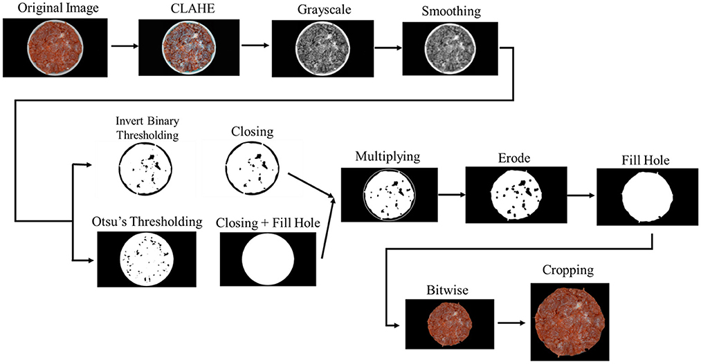
Figure 4. The flow of image segmentation. Sample images were enhanced using CLAHE. Segmentation stages were conducted using Otsu threshold, calculating the T threshold automatically based on the input images.

Color feature extraction

The color composition of an image is related to the probability of color distribution. A probability distribution can be characterized by its moments. The image color distribution is interpreted as a probability distribution. Color moments can be used to characterize the color distribution (Afifi and Ashour, 2012). In this study, there are 24 color features extracted from the image. The color space RGB and CIE L^*a^*b are used. The RGB color space is the most commonly used color space, which determines the value of the Red-Green-Blue of an image. While CIE L^*a^*b determines the value of L (lightness) associated with illumination, then a and b determine the value of magenta-green and yellow-blue, respectively (Gonzalez et al., 2009; Afifi and Ashour, 2012). The color moments were extracted at every single channel at each color space, including the mean, standard deviation, skewness, and kurtosis (Afifi and Ashour, 2012). If the i_th channel in the j-th image pixel is represented as P_ij and N is the total number of pixels of the image. The mean (M_i), standard deviation (SD_i), skewness (SK_i), and kurtosis K_i) color moments can be represented in Table 1, respectively.

TABLE 1

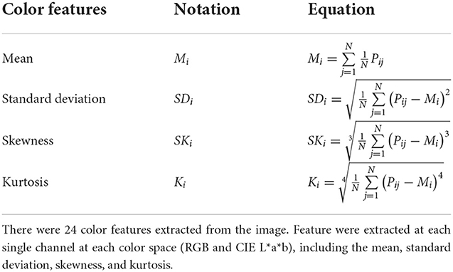
Table 1. Color features.

Textural feature extraction

Textural features are obtained based on the gray-level co-occurrence matrix (GLCM) by considering the intensity distribution and the spatial position of two neighboring pixels in an image. That is, The GLCM represents the frequency formation of the pixel pairs. The textural features extracted in this study were adapted from the work of Haralick et al. (1973). The image's GLCM is expressed as a matrix n x n, which represents the grayscale values. The matrix element depends on the two specified pixel frequencies (Öztürk and Akdemir, 2018). Both pixel pairs can vary depending on their neighborhood. As shown in Table 2, there were 14 extracted features used in this study, such as angular second moment, contrast, correlation, variance, inverse difference moment, sum of average, sum of variance, sum of entropy, entropy, difference of variance, different of entropy, information of measures correlation 1, information of measures correlation 2 and maximal correlation difference.

TABLE 2

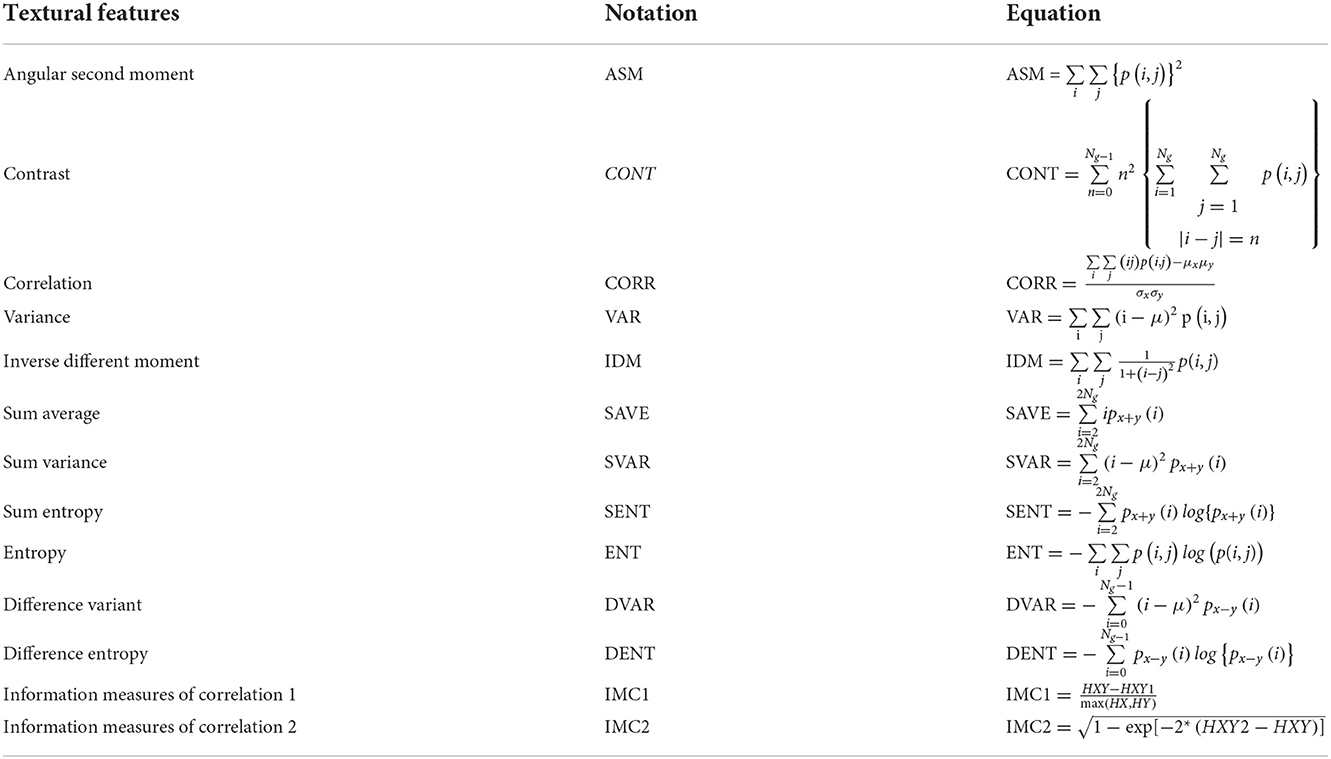
Table 2. The textural features computed from GLCMs.

Here, p(i, j) is the GLCM value at the (i, j) spatial coordinates; N_g is gray tone or the gray level of the co-occurrence matrix; μ_x, μ_y are mean of p_x(i) and p_y(j), respectively; and σ_x and σ_y are the variance of p_x(i) and p_y(j), respectively. The parameters for textural features, as shown in Table 2, can be calculated from the following Equations (1)–(5).

$\begin{array}{ll}{p}_x(i)={\displaystyle \sum _{j=1}^{2N_g}}p(i,j)& (1)\end{array}$

$\begin{array}{ll}{p}_y(i)={\displaystyle \sum _{i=1}^{N_g}}(i,j)& (2)\end{array}$

$\begin{array}{ll}HXY=-{\displaystyle \sum _i}{\displaystyle \sum _j}p(i,j)log(p(i,j))& (3)\end{array}$

$\begin{array}{ll}HXY1=-{\displaystyle \sum _i}{\displaystyle \sum _j}p(i,j)log\left\{p_x(i)p_y\left(j\right)\right\}& (4)\end{array}$

$\begin{array}{ll}HXY2=-{\displaystyle \sum _i}{\displaystyle \sum _j}{p}_x(i)p_y\left(j\right)log\left\{p_x(i)p_y\left(j\right)\right\}& (5)\end{array}$

DNN model development

DNN is an artificial neural network (ANN) with multilayer perceptron with many hidden layers. The DNN is generally feed forward networks (FFNNs) in which data goes from the input layer to the output layer without returning backward. It usually consists of a fully connected layer, where this fully connected layer consists of standard neurons that connect each input element to each output element with a different weight (Sunil et al., 2021). Figure 5 shows a proposed DNN model architecture with the extracted features used as input. This model consists of four blocks of fully connected layers and a classifier. Each block has a dense layer with an activation function. The dropout was used to fix the overfitting issue, and batch normalization was used to quicken training. The input layer, together with every stage feature in each block, is concatenated to be the block feature. The proposed DNN parameters used in this study are shown in Table 3.

FIGURE 5

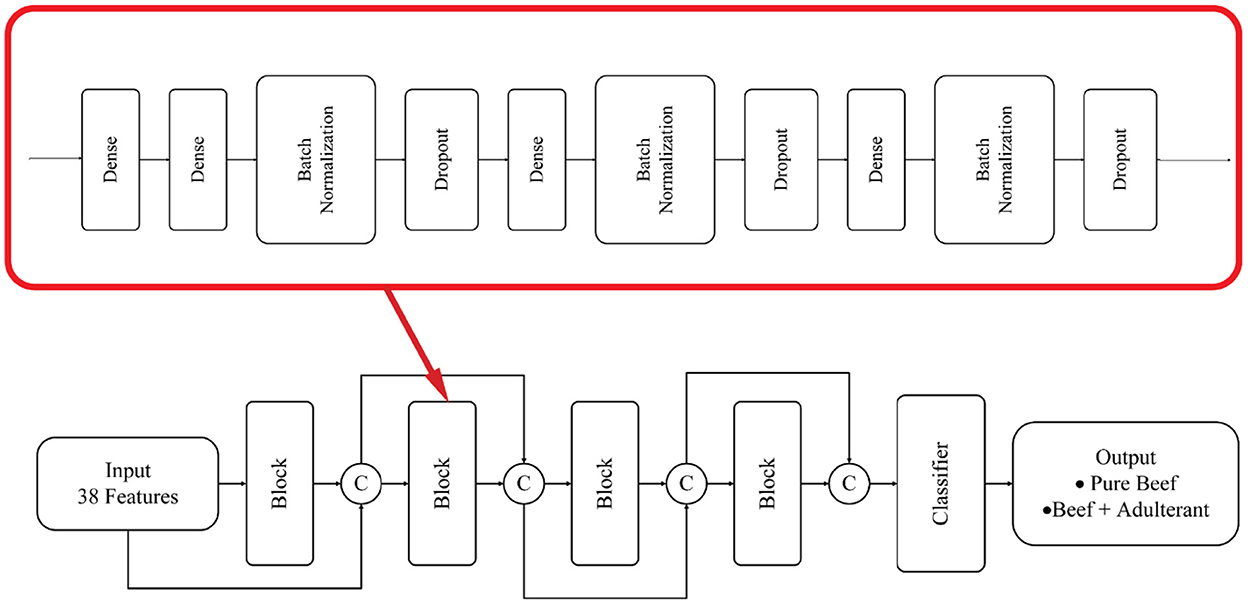
Figure 5. The proposed DNN architecture. This model consists of four blocks fully connected layer and a classifier. Each block has a dense layer with an activation function. Dropout was used to address the overfitting and batch normalization was used to gain learning speed during training process.

TABLE 3

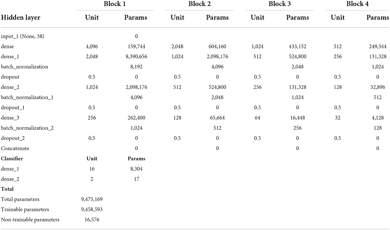
Table 3. The proposed DNN parameters.

Activation functions and optimizers are an important part of a neural network design (Hayou et al., 2019; Wang et al., 2022). In the first stage, 56 DNN models were investigated with several activation functions and optimizers. This investigation aimed to find the best activation function for the classifier and the optimizers to get the best performance (higher accuracy and lower loss). Activation functions and optimizers are an essential part of the design of a neural network (Hayou et al., 2019; Wang et al., 2022). The activation function in the hidden layer control the training dataset's network model. The activation function in the output layer will define the type of model prediction. Seven activation functions of the classifier were to be investigated, including sigmoid, softplus, tanh, selu, exponential, LeakyReLU, and softmax. There were seven activation functions of classifier, including sigmoid, softplus, tanh, selu, exponential, LeakyReLU, and softmax, and there were eight optimizers, including SGD, Adam (Kingma and Ba, 2014), RMSprop, Adadelta (Zeiler, 2012), Adagrad (Lydia and Francis, 2019), Adamax, Nadam, and Follow The Regularized Leader (FTRL) were investigated. In the next stage, our proposed DNN is compared to others well-known classifiers such as (k-nearest neighbors' algorithm (KNN), Logistic Regression (LR), Decision Tree (DT), Random Forest (RF), Adaptive Boosting (AdaBoost), and Support Vector Machine (SVM) (Bolón-Canedo and Remeseiro, 2020). The performance of the classifier is evaluated based on its accuracy, sensitivity, and precision.

The experiments were carried out on 500 samples of segmented images, including 250 pure minced beef and 250 adulterated minced beef. The samples were divided into three subsets, the training set was 70% of all samples stratified by the labels, the validation set was 10% of the training set, and the testing set was 30% of all samples. The data set was divided into three subsets because, in small data sets, an additional split could result in a smaller training set that is more susceptible to overfitting (Miraei Ashtiani et al., 2021). The training and validation datasets are used together to develop the classification model and the testing is used solely for testing the final results. After the model training stage, an evaluation will be carried out using the testing set.

Feature importance analysis

In this study, there were 38 extracted image features, including 24 color and 14 textural features. The color and textural features could be used separately as input for the classification. Feature importance analysis was performed by calculating SHAP (Shapley Additive exPlanations) value. The SHAP value can compute the degree of influence of each feature on the output value. The SHAP value is defined as the value for the co-expected value function of the machine learning model (Lee et al., 2022). The main idea of SHAP is to calculate the Shapley value for each sample feature to be interpreted, where each Shapley value represents the impact that the associated feature has on the prediction. Features with high Shapley values have a more significant impact, and features with low Shapley values have less impact concerning the prediction. In the conventional method, the importance of a feature is calculated by averaging the absolute values of the SHAP values for all instances.

SHAP is introduced by Lundberg and Lee in 2017 to interpret machine learning models through Shapley value (Lundberg and Lee, 2017). The Shapley value implies the average contribution of a feature to a prediction, proposed by Lloyd Shapley in 1953 (Shapley, 2016). Shapley value can be represented in Equations (6).

$\begin{array}{ll}{\varphi }_i={\displaystyle \sum _{S\subseteq F}}\frac{|S|!(|F|-|S|-1)!}{|F|!}\left[f_{S\cup \{i\}}(x_{S\cup \{i\}})-f_S(x_s)\right]& (6)\end{array}$

Here, ϕ_i is the Shapley value for feature i, S is the subset of the feature set F. Then, it will be iterated as much as the combination of _FC_S. The f_S∪{i}(x_S∪{i}) − f_S(x_s) is marginal value, where f_S∪{i} is the prediction of model f with the feature i presents and f_S is the model with feature i does not change, but the other feature is given random value from dataset F. While x_S represented the value of input feature in subset S SHAP used simpler model to explain more complex model. The simpler model is the interpretation of the real model. This explanation model can be expressed as the Equation (7).

$\begin{array}{ll}g\left(z^{\prime }\right)={\varphi }_0+{\displaystyle \sum _{i=1}^M{\varphi }_i{z}_i}& (7)\end{array}$

Here, g is the explanation model and z' is the feature input. Whereas, ϕ₀ is the mean of model prediction result.

Performance models evaluation and analysis

Predictions will be made on the testing set using a pre-trained model in this evaluation process. In this study, the metrics used to evaluate model performance are accuracy, precision, and sensitivity (recall). These metric values can be obtained by Equations (8)–(10) (Javanmardi et al., 2021).

$\begin{array}{ll}\text{Accuracy}=\frac{TP+TN}{TP+TN+FP+FN}& (8)\end{array}$

$\begin{array}{ll}\text{Sensitivity}=\frac{TP}{TP+FN}& (9)\end{array}$

$\begin{array}{ll}\text{Precision}=\frac{TP}{TP+FP}& (10)\end{array}$

where, TP, TN, FP, and FN are true positive, true negative, false positive, and false negative, respectively.

Results and discussion

DNN training and validation accuracy

Figure 6 shows the training and validation accuracy and loss of the DNN classifier over 200 training epochs (x-axis) for each dataset. Each plot shows the first cross-validation run representatives for all ten runs. Figure 6A shows train learning curve which is generated from the training dataset that gives an insight of how effectively the model is learning. Figure 6B shows the validation learning curve which is generated from a hold-out validation dataset that gives an idea of how well the model is generalizing. The classification accuracy values obtained by DNN showed that combined color and texture features yielded results up to 98.00%. Figure 7 shows a confusion matrix, a summary of prediction results on a classification based on the validation dataset. By using the color feature, only 10 cases were found that were misclassified. By using the texture feature, only seven cases were found that were misclassified. By using the combined features, only three cases were found that were misclassified. It shows that model with combined color and texture features as input has better training and validation accuracy than others. A lower loss indicates a better-performing model. It also can be seen that the model did not tend to ovefit. The model demonstrates a smooth curve and converges after 200 training epochs.

FIGURE 6

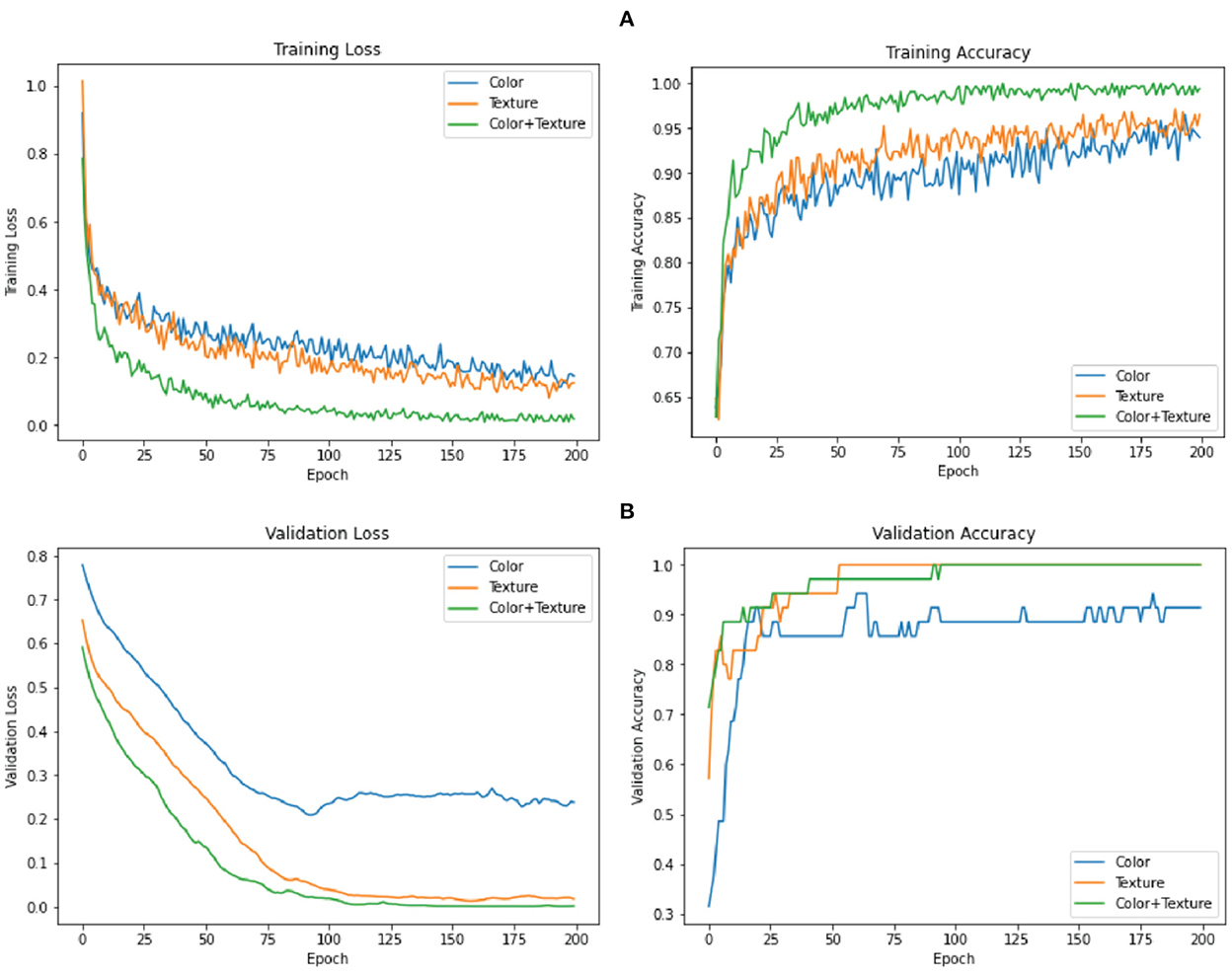
Figure 6. Plots of training (A) and validation (B) performance. Blue, orange, and green lines indicate the model loss and accuracy for color, textural, and both, respectively.

FIGURE 7

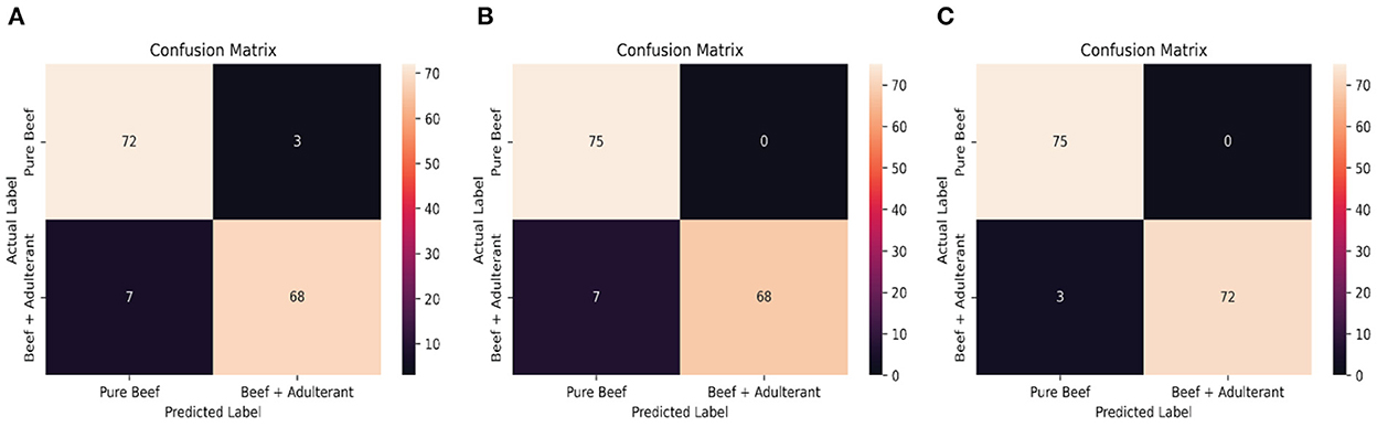
Figure 7. The confusion matrix of classification results. Confusion matrix is a very popular measure parameter used while solving classification problems. Confusion matrix represent counts from predicted and actual values. Here, (A–C) indicate the classification result based on color, textural, and color and textural features, respectively.

Selection of DNN model architecture

The classification performance of the model is shown in Table 4. Overall, the DNN model with Softmax activation function for classifier has the best performance in terms of accuracy, up to 86%. These results indicate that Softmax significantly outperformed other functions at higher learning rates. Softmax achieves an accuracy of 99.33% with Adam, RMSProp, SGD, and Adagrad, which are significantly superior to the accuracy rates of the other activation functions. Thus, with any optimizer, Softmax performed better than any other activation function. The obtained results also show that the FTRL and AdaDelta gradient algorithms, present the lowest performances.

TABLE 4

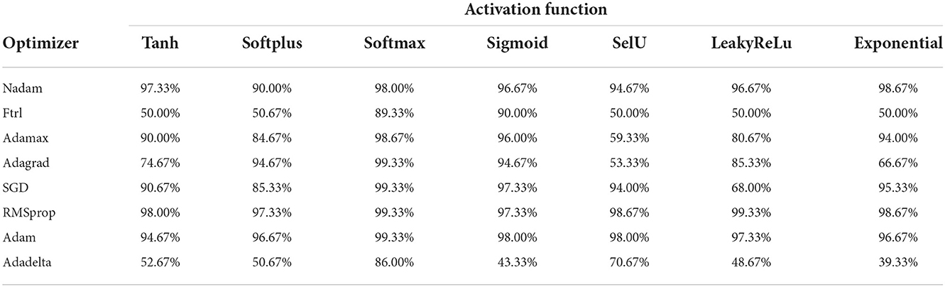
Table 4. The classification performance of DNN models based on its accuracies.

As shown in Table 4, most of the DNN models with various optimizer functions show high accuracy, except the model with Adadelta and Ftrl optimizer. The RMSProp optimizer performs better according to the loss value, which is 0.007, the lowest value, as shown in Table 5. Based on the results, the DNN model with Softmax activation function for the classifier and RMSprop optimizer was chosen and used in the following steps. Choosing the right optimizer and activation function produce a better model.

TABLE 5

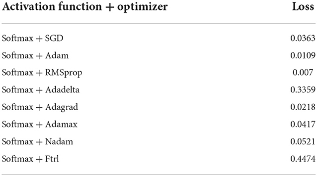
Table 5. The loss value of DNN models with softmax activation function.

DNN performance compared with others

The proposed DNN has been compared with six machine learning algorithms. Classification results for pure or adulterated minced beef using six machine-learning models are summarized in Table 6. Overall, the DNN classifier yielded better performance than others. Classification accuracy values obtained by DNN showed that combined color and texture features yielded results as high as 98.00%. Moreover, there was not much difference in the result between all classifiers with textual features as input. All the results demonstrate that the multiple-modality (color and textural) feature could efficiently improve the classification model performance in each machine-learning algorithm.

TABLE 6

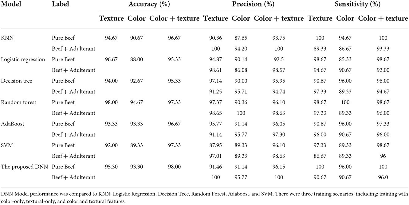
Table 6. The DNN model performance.

The results show that the overall precision of models was 88–98%. Using all features, the individual classification precision in DNN was 96.15% for pure minced beef samples and 100% for adulterated minced beef samples. For only textural features, the precision values were 91.46% for pure and 100% for adulterated samples. The classifier is also highly sensitive. Using all features, the individual classification sensitivity in DNN were 100% for pure samples and 96% for adulterated samples. Based on accuracy, precision, and sensitivity, we clearly perceive that our proposed DNN obtained better results compared to others.

Feature importance analysis

Figure 8 below shows the distribution of the SHAP value calculated with the testing set. Color and textural features are sorted by their importance and stacked vertically. A higher value indicated higher importance. For each feature, the color of the points is determined by the value of the same feature. The higher feature values are redder. The results show the 15 top impacting features on the trained DNN model. It shows that the textural features have more impact on prediction results. The importance of GLCM features was confirmed by previous studies (Rady et al., 2021). Based on the results, we also understood the nature of these feature-prediction relationships. For example, the higher values of Correlation and Sum Average seems to have the directly relationship. It means that larger values for this feature are associated with higher SHAP values. In contrast, for Sum Entropy, Contrast, and Inverse Different Moment notice how as the feature value increases the SHAP values decrease. This tells us that the smaller values of these features for will lead to a higher prediction result.

FIGURE 8

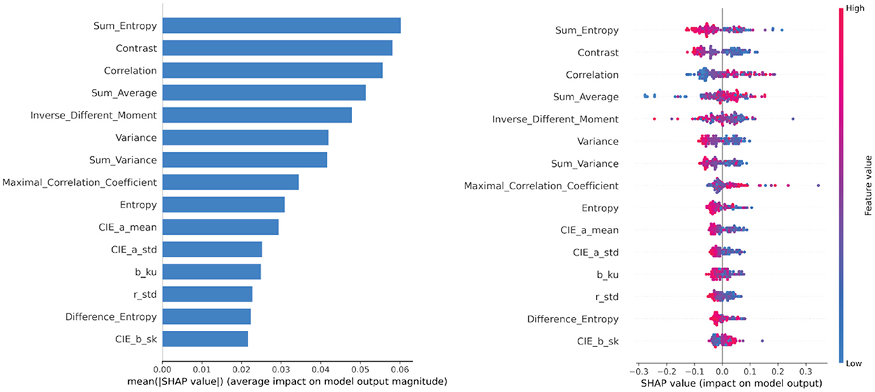
Figure 8. Feature importance based on SHAP values. On the left side, the mean absolute SHAP values are calculated, to illustrate global feature importance and determine top 15 impacting features. On the right side, the local explanation summary shows the direction of the relationship between features and adulteration detection. A positive SHAP value means contribution to pure minced beef and a negative SHAP value means the opposite.

DNN model with selected feature

We investigated 5, 10, and 15 selected features based on the SHAP feature importance analysis. Overall, there was no significant gap between DNN with all color and textural features and selected features. Table 7 shows the DNN model performance with all and selected features. Figure 9 below shows the confusion matrix of classification. While various features did not significantly differ in classification performance, the selected features yielded higher performance and faster training and testing time. When the number of selected features was reduced to 5, it turned out that the model did not perform well. The results show that textural features have a more significant impact than color features. However, we still recommend using the color feature as input during model development. This is supported by the contribution of five color features in the top 15 impacting features as shown in Figure 8.

TABLE 7

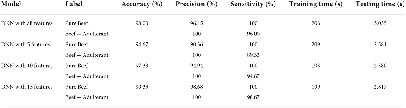
Table 7. The performance of DNN model with selected features.

FIGURE 9

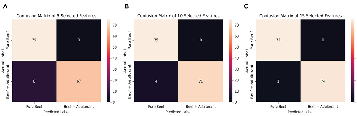
Figure 9. The confusion matrix of selected features, (A) 5 features, (B) 10 features, (C) 15 features.

The DNN model with 15 features is the best model with the highest accuracy (99.33%), precision (up to 98.68%), sensitivity (up to 98.67%), and the training and testing time are also faster than the DNN model with all features. Training and testing time are decreasing the lesser the features used in the model, but while using five features, the training time is longer than the model with all features. But the difference in testing time is not really significant with just several milliseconds. There is an increase in accuracy when using only 15 features compared to all features. Without feature selection, the accuracy of DNN reached 98 or 1.7% greater than SVM, which was ranked second. Sensitivity of DNN in detecting pure samples reaches 100%, is as good as KNN, and is better than other algorithms. Meanwhile, sensitivity of DNN in detecting adulterated samples reaches 96%, comparable to other algorithms. In terms of precision, DNN is superior to others, reaching 100% in detecting pure samples and 96.15% in detecting adulterated samples. With feature selection, the performance of DNN is better, with accuracy increasing by 1.3%, sensitivity increasing by 2.53%, and precision increasing by 2.67%. In addition to accuracy, precision, and sensitivity, the training and testing times in particular are also significant performance measures. In this evaluation, the training and testing time are quite fast. The testing time is the overall amount of time needed for computations, such as preprocessing, feature extraction, and model evaluation. The training time is the amount of time needed for a model to train on a dataset. Table 7 displays the training and testing times for DNN algorithm with feature selection. In this study, there was no significant difference of training and testing times. The training and testing times of the DNN algorithm with 15 selected features are 199 and 2.817 s, respectively.

The classification performance of proposed system is better than the other studies that used spectroscopic systems (Weng et al., 2020; Fengou et al., 2021), multispectral imaging systems (Ropodi et al., 2015), and color imaging systems (Rady et al., 2021; Ningsih et al., 2022), in terms of accuracy, precision, and sensitivity, for meat adulteration detection. The use of DNN shows better results when compared to other machine algorithms, as well as LDA algorithm from the previous related work by Rady et al. (2021). However, the proposed system performance is still inferior to hyperspectral imaging in terms of accuracy (Rady and Adedeji, 2020). Hyperspectral imaging could achieve classification accuracies of 100%, but it utilizes large and costly systems, which differ from our work. Our proposed system was developed with low-cost components, such as a LED-based illuminator and a consumer camera, with a total cost of only US$ 300. The proposed technology is also user-friendly. It does not require highly-skilled users to operate. Users just need to capture the image samples, run the image processing algorithm as well as the DNN classifier, and get the classification results. As show in Table 7, it is also fast in detecting adulteration, approximately 193–209 s for training and 2–3 s for testing. Thus, it could be integrated into a cloud-based IoT system that can offer assurance to several supply chain stakeholders, including consumers and regulatory authorities.

Conclusion

This work deals with the feasibility of using low-cost imaging system coupled with DNN for adulteration detection in minced beef. The DNN classifier was developed, investigated, and compared with well-known machine learning algorithm. The result showed that the DNN classifier yielded better performance than others. The DNN performed best, with individual accuracy, precision, and sensitivity up to 99.33, 98.68, and 98.67%, respectively. However, the system presented in this study can only be used to detect surface adulterants in minced beef. Moreover, the performance of the DNN models could be improved by training a more extensive data set. Advanced machine learning algorithms, such as convolution neural networks, could be used to optimize the model classifier. In future work, we plan to apply diverse deep learning algorithms on larger datasets with diversity in meat sources, origins, and storage conditions. Additionally, the proposed system could be integrated into an Internet of Things (IoT) cloud system that can assure stakeholders of the minced beef supply chain.

Data availability statement

The raw data supporting the conclusions of this article will be made available by the authors, without undue reservation.

Author contributions

AH and IS conceived the study, participated in its design, analyzed the results, and wrote the manuscript. WW collected and interpreted the raw data. SK, SS, and NA implemented the methods and performed the experiments. All authors read and approved the final manuscript.

Funding

The research has been funded by the Indonesian Government, Kementerian Pendidikan, Kebudayaan, Riset, dan Teknologi (Ministry of Education, Culture, Research, and Technology) for supporting this work under project scheme University's Competitive Fundamental Research Program (Grant No. 084/E5/PG.02.00.PT/2022 with an institutional contract No. 1366/PKS/ITS/2022).

Conflict of interest

The authors declare that the research was conducted in the absence of any commercial or financial relationships that could be construed as a potential conflict of interest.

Publisher's note

All claims expressed in this article are solely those of the authors and do not necessarily represent those of their affiliated organizations, or those of the publisher, the editors and the reviewers. Any product that may be evaluated in this article, or claim that may be made by its manufacturer, is not guaranteed or endorsed by the publisher.

References

Afifi, A. J., and Ashour, W. M. (2012). Image retrieval based on content using color feature. ISRN Comp. Graph. 2012, e248285. doi: 10.5402/2012/248285

CrossRef Full Text | Google Scholar

Al-Sarayreh, M., Reis, M. M., Yan, W. Q., and Klette, R. (2020). Potential of deep learning and snapshot hyperspectral imaging for classification of species in meat. Food Control 117, 1–12. doi: 10.1016/j.foodcont.2020.107332

CrossRef Full Text | Google Scholar

Asmara, R. A., Romario, R., Batubulan, K. S., Rohadi, E., Siradjuddin, I., Ronilaya, F., et al. (2018). Classification of pork and beef meat images using extraction of color and texture feature by grey level co-occurrence matrix method. IOP Conf. Ser.: Mater. Sci. Eng. 434, 012072. doi: 10.1088/1757-899X/434/1/012072

CrossRef Full Text | Google Scholar

Ballin, N. Z. (2010). Authentication of meat and meat products. Meat Sci. 86, 577–587. doi: 10.1016/j.meatsci.2010.06.001

PubMed Abstract | CrossRef Full Text | Google Scholar

Beganović, A., Hawthorne, L. M., Bach, K., and Huck, C. W. (2019). Critical review on the utilization of handheld and portable raman spectrometry in meat science. Foods 8, E49. doi: 10.3390/foods8020049

PubMed Abstract | CrossRef Full Text | Google Scholar

Bolón-Canedo, V., and Remeseiro, B. (2020). Feature selection in image analysis: a survey. Artif. Intell. Rev. 53, 2905–2931. doi: 10.1007/s10462-019-09750-3

CrossRef Full Text | Google Scholar

Du, C. J., Sun, D. W., Jackman, P., and Allen, P. (2008). Development of a hybrid image processing algorithm for automatic evaluation of intramuscular fat content in beef M. longissimus dorsi. Meat Sci. 80, 1231–1237. doi: 10.1016/j.meatsci.2008.05.036

PubMed Abstract | CrossRef Full Text | Google Scholar

Erwanto, Y., Rohman, A., Zainal Abidin, M., and Ariyani, D. (2012). Pork Identifi cation Using PCR-RFLP of Cytochrome b Gene and Species Specifi c PCR of Amelogenin Gene. Agritech. 32, 370–377. doi: 10.22146/agritech.9579

CrossRef Full Text | Google Scholar

European Parliament (2014). European Parliament Resolution of 14 January 2014 on the Food Crisis, Fraud in the Food Chain and the Control Thereof (2013/2091(INI)). Available online at: http://ec.europa.eu/food/food/horsemeat/plan_en.htm (accessed August 2, 2022).

Google Scholar

Feng, C. H., Makino, Y., Oshita, S., and García Martín, J. F. (2018). Hyperspectral imaging and multispectral imaging as the novel techniques for detecting defects in raw and processed meat products: current state-of-the-art research advances. Food Control 84, 165–176. doi: 10.1016/j.foodcont.2017.07.013

CrossRef Full Text | Google Scholar

Fengou, L. C., Lianou, A., Tsakanikas, P., Mohareb, F., and Nychas, G. J. E. (2021). Detection of meat adulteration using spectroscopy-based sensors. Foods 10, 1–13. doi: 10.3390/foods10040861

PubMed Abstract | CrossRef Full Text | Google Scholar

Geiker, N. R. W., Bertram, H. C., Mejborn, H., Dragsted, L. O., Kristensen, L., Carrascal, J. R., et al. (2021). Meat and human health—Current knowledge and research gaps. Foods 10, 1556. doi: 10.3390/foods10071556

PubMed Abstract | CrossRef Full Text | Google Scholar

Gonzalez, R. C., Woods, R. E., and Masters, B. R. (2009). Digital image processing, third edition. J. Biomed. Opt. 14, 029901. doi: 10.1117/1.3115362

CrossRef Full Text | Google Scholar

Haralick, R. M., Shanmugam, K., and Dinstein, I. (1973). Textural features for image classification. IEEE Transact. Syst. Man Cybernet. SMC-3, 610–621. doi: 10.1109/TSMC.1973.4309314

CrossRef Full Text | Google Scholar

Hayou, S., Doucet, A., and Rousseau, J. (2019). “On the Impact of the Activation Function on Deep Neural Networks Training,” in 36th International Conference on Machine Learning (Long Beach, CA: Proceedings of Machine Learning Research), 2672–2680. doi: 10.48550/arXiv.1902.06853

CrossRef Full Text | Google Scholar

Hwang, H., Park, B., Nguyen, M., and Chen, Y.-R. (1997). Hybrid image processing for robust extraction of lean tissue on beef cut surfaces. Comp. Electron. Agric. 17, 281–294. doi: 10.1016/S0168-1699(97)01321-5

CrossRef Full Text | Google Scholar

Javanmardi, S., Miraei Ashtiani, S.-H., Verbeek, F. J., and Martynenko, A. (2021). Computer-vision classification of corn seed varieties using deep convolutional neural network. J. Stored Prod. Res. 92, 101800. doi: 10.1016/j.jspr.2021.101800

CrossRef Full Text | Google Scholar

Kamruzzaman, M. (2021). Fraud detection in meat using hyperspectral imaging. Meat Muscle Biol. 5, 1–10. doi: 10.22175/mmb.12946

CrossRef Full Text | Google Scholar

Kingma, D. P., and Ba, J. (2014). “Adam: A Method for Stochastic Optimization,” in International Conference on Learning Representations 2015 (San Diego, CA). doi: 10.48550/arXiv.1412.6980

CrossRef Full Text | Google Scholar

Kumar, Y., and Chandrakant Karne, S. (2017). Spectral analysis: a rapid tool for species detection in meat products. Trends Food Sci. Technol. 62, 59–67. doi: 10.1016/j.tifs.2017.02.008

PubMed Abstract | CrossRef Full Text | Google Scholar

Lee, Y.-G., Oh, J.-Y., Kim, D., and Kim, G. (2022). SHAP value-based feature importance analysis for short-term load forecasting. J. Electr. Eng. Technol. doi: 10.1007/s42835-022-01161-9

CrossRef Full Text | Google Scholar

Liu, D., and Yu, J. (2009). “Otsu method and K-means,” in 2009 Ninth International Conference on Hybrid Intelligent Systems, 344–349.

Google Scholar

Liu, Y., Pu, H., and Sun, D.-W. (2017). Hyperspectral imaging technique for evaluating food quality and safety during various processes: a review of recent applications. Trends Food Sci. Technol. 69, 25–35. doi: 10.1016/j.tifs.2017.08.013

CrossRef Full Text | Google Scholar

Lundberg, S., and Lee, S.-I. (2017). A Unified Approach to Interpreting Model Predictions. Available online at: http://arxiv.org/abs/1705.07874 (accessed September 7, 2022).

Google Scholar

Lydia, A. A., and Francis, F. S. (2019). Adagrad - an optimizer for stochastic gradient descent. Int. J. Inf. Comput. Sci. 6, 566–568.

Google Scholar

Miraei Ashtiani, S.-H., Javanmardi, S., Jahanbanifard, M., Martynenko, A., and Verbeek, F. J. (2021). Detection of mulberry ripeness stages using deep learning models. IEEE Access 9, 100380–100394. doi: 10.1109/ACCESS.2021.3096550

CrossRef Full Text | Google Scholar

Ningsih, L., Buono, A., and Haryanto, T. (2022). Fuzzy learning vector quantization for classification of mixed meat image based on character of color and texture. J. Rekayasa Sist. Teknol. Inf. 6, 421–429. doi: 10.29207/resti.v6i3.4067

CrossRef Full Text | Google Scholar

Otsu, N. (1979). A threshold selection method from gray-level histograms. IEEE Trans. Syst. Man Cybern. 9, 62–66. doi: 10.1109/TSMC.1979.4310076

CrossRef Full Text | Google Scholar

Öztürk, S., and Akdemir, B. (2018). Application of feature extraction and classification methods for histopathological image using GLCM, LBP, LBGLCM, GLRLM and SFTA. Proc. Comput. Sci. 132, 40–46. doi: 10.1016/j.procs.2018.05.057

CrossRef Full Text | Google Scholar

Pizer, S. M., Amburn, E. P., Cromartie, R., and Geselowit, A. (1987). Adaptive Histogram Equalization And Its Variations. Comput. Gr. Image Process. 39, 355–368. doi: 10.1016/S0734-189X(87)80186-X

CrossRef Full Text | Google Scholar

Premanandh, J. (2013). Horse meat scandal - A wake-up call for regulatory authorities. Food Control 34, 568–569. doi: 10.1016/j.foodcont.2013.05.033

CrossRef Full Text | Google Scholar

Rady, A., and Adedeji, A. (2018). Assessing different processed meats for adulterants using visible-near-infrared spectroscopy. Meat Sci. 136, 59–67. doi: 10.1016/j.meatsci.2017.10.014

PubMed Abstract | CrossRef Full Text | Google Scholar

Rady, A., and Adedeji, A. A. (2020). Application of hyperspectral imaging and machine learning methods to detect and quantify adulterants in minced meats. Food Anal. Methods 13, 970–981. doi: 10.1007/s12161-020-01719-1

CrossRef Full Text | Google Scholar

Rady, A. M., Adedeji, A., and Watson, N. J. (2021). Feasibility of utilizing color imaging and machine learning for adulteration detection in minced meat. J. Agric. Food Res. 6, 100251. doi: 10.1016/j.jafr.2021.100251

CrossRef Full Text | Google Scholar

Reis, M. M., Van Beers, R., Al-Sarayreh, M., Shorten, P., Yan, W. Q., Saeys, W., et al. (2018). Chemometrics and hyperspectral imaging applied to assessment of chemical, textural and structural characteristics of meat. Meat Sci. 144, 100–109. doi: 10.1016/j.meatsci.2018.05.020

PubMed Abstract | CrossRef Full Text | Google Scholar

Roberts, J., Power, A., Chapman, J., Chandra, S., and Cozzolino, D. (2018). A short update on the advantages, applications and limitations of hyperspectral and chemical imaging in food authentication. Appl. Sci. 8, 505. doi: 10.3390/app8040505

CrossRef Full Text | Google Scholar

Ropodi, A. I., Pavlidis, D. E., Mohareb, F., Panagou, E. Z., and Nychas, G. J. E. (2015). Multispectral image analysis approach to detect adulteration of beef and pork in raw meats. Food Res. Int. 67, 12–18. doi: 10.1016/j.foodres.2014.10.032

CrossRef Full Text | Google Scholar

Shapley, L. S. (2016). “A value for n-person games,” in A Value for n-Person Games (Princeton, NJ: Princeton University Press), 307–318. doi: 10.1515/9781400881970-018

CrossRef Full Text | Google Scholar

Silva, L. C. R., Folli, G. S., Santos, L. P., Barros, I. H. A. S., Oliveira, B. G., Borghi, F. T., et al. (2020). Quantification of beef, pork, and chicken in ground meat using a portable NIR spectrometer. Vib. Spectrosc. 111, 103158. doi: 10.1016/j.vibspec.2020.103158

CrossRef Full Text | Google Scholar

Soille, P. (2004). “Opening and closing,” in Morphological Image Analysis: Principles and Applications, ed P. Soille (Berlin, Heidelberg: Springer), 105–137.

Google Scholar

Song, W., Yun, Y. H., Wang, H., Hou, Z., and Wang, Z. (2021). Smartphone detection of minced beef adulteration. Microchem. J. 164, 106088. doi: 10.1016/j.microc.2021.106088

CrossRef Full Text | Google Scholar

Sunil, G., Saidul Md, B., Zhang, Y., Reed, D., Ahsan, M., Berg, E., et al. (2021). Using deep learning neural network in artificial intelligence technology to classify beef cuts. Front. Sens. 2, 654357. doi: 10.3389/fsens.2021.654357

CrossRef Full Text | Google Scholar

Swartidyana, F. R., Yuliana, N. D., Adnyane, I. K. M., Hermanianto, J., and Jaswir, I. (2022). Differentiation of beef, buffalo, pork, and wild boar meats using colorimetric and digital image analysis coupled with multivariate data analysis. J. Teknol. Ind. Pangan 33, 87–99. doi: 10.6066/jtip.2022.33.1.87

CrossRef Full Text | Google Scholar

Wahyuni, H., Vanany, I., and Ciptomulyono, U. (2019). Food safety and halal food in the supply chain: Review and bibliometric analysis. J. Ind. Eng. Manag. 12, 373–391. doi: 10.3926/jiem.2803

CrossRef Full Text | Google Scholar

Wang, X., Ren, H., and Wang, A. (2022). Smish: a novel activation function for deep learning methods. Electronics 11, 540. doi: 10.3390/electronics11040540

CrossRef Full Text | Google Scholar

Weng, S., Guo, B., Tang, P., Yin, X., Pan, F., Zhao, J., et al. (2020). Rapid detection of adulteration of minced beef using Vis/NIR reflectance spectroscopy with multivariate methods. Spectrochimica Acta 230, 118005. doi: 10.1016/j.saa.2019.118005

PubMed Abstract | CrossRef Full Text | Google Scholar

Zeiler, M. D. (2012). ADADELTA: an adaptive learning rate method. arXiv e-prints. doi: 10.48550/arXiv.1212.5701

CrossRef Full Text | Google Scholar

Zheng, X., Li, Y., Wei, W., and Peng, Y. (2019). Detection of adulteration with duck meat in minced lamb meat by using visible near-infrared hyperspectral imaging. Meat Sci. 149, 55–62. doi: 10.1016/j.meatsci.2018.11.005

PubMed Abstract | CrossRef Full Text | Google Scholar