Coupling optical and SAR imagery for automatic garlic mapping

Accurate garlic identification and mapping are vital for precise crop management and the optimization of yield models. However, previous understandings of garlic identification were limited. Here, we propose an automatic garlic mapping framework using optical and synthetic aperture radar (SAR) images on the Google Earth Engine. Specifically, we firstly mapped winter crops based on the phenology of winter crops derived from Sentinel-2 data. Then, the garlic was identified separately using Sentinel-1 and Sentinel-2 data based on the winter crops map. Additionally, multi-source validation data were used to evaluate our results. In garlic mapping, coupled optical and SAR images (OA 95.34% and kappa 0.91) outperformed the use of only optical images (OA 74.78% and kappa 0.50). The algorithm explored the potential of multi-source remote sensing data to identify target crops in mixed and fragmented planting regions. The garlic planting information from the resultant map is essential for optimizing the garlic planting structure, regulating garlic price fluctuations, and promoting a healthy and sustainable development of the garlic industry.

Introduction

Garlic is one of the primary economic crops (e.g., garlic, peanut, rape, sugar beet, sugarcane, and cotton) in China. According to statistics from the United Nations Food and Agriculture Organization (FAOSTAT, 2020), garlic production in China reached 23.30 million tons in 2019, which made China the largest garlic planting and production region in the world. Due to the small area and scattered distribution of garlic crops, few studies have been able to map them accurately, which hinders their precise management (Zhang et al., 2019; Guo et al., 2022b).

Traditionally, information about the garlic planting area is mainly obtained based on a sampling or field survey. Such methods are not only vulnerable to subjective factors (Liu et al., 2018a) but they also have a long cycle, are labor-intensive, and are time-consuming (Siyal et al., 2015; Verma et al., 2017). Satellite imagery has become a viable crop mapping data source, due to its high mapping efficiency and low cost (Massey et al., 2017; Vallentin et al., 2021; Guo et al., 2022a), and it is widely used in many fine-mapping fields, such as urban land mapping (Liu et al., 2018b), water surface area change (Xia et al., 2019; Zhao et al., 2022), forest degradation (Bullock et al., 2020), cropland classification (Poortinga et al., 2019), and wetland classification (Amani et al., 2019).

At present, the accuracy of the garlic extraction based on remote sensing data is mostly unsatisfactory. Qu et al. (2021) attempted to map garlic distribution using the threshold method and Landsat images. However, the limited temporal resolution of the Landsat satellite makes it difficult to obtain sufficient high-quality images during the growing season, which can easily ignore spectral differences of crops. Therefore, the accuracy and timeliness of the results are difficult to guarantee. Lee et al. (2015) attempted to use ultra-high-resolution Worldview-2 satellite images to map garlic distribution. However, the high cost and limited coverage of a single image restrict their application to a large region. Similarly, although Unmanned Aerial Vehicle (UAV) imagery provides more spatial details, it usually requires many images to fully cover the study area and is difficult to apply to large areas. The Sentinel-2 (S2) imagery provided a temporal resolution of 5 days and a spatial resolution of 10 m, providing an opportunity for the identification of broken and scattered garlic distributions.

The quality of Sentinel-1 (S1) imagery is independent of weather conditions (Du et al., 2015; Oyoshi et al., 2016), which compensates for the lack of optical observations due to bad weather during the crop growth cycle (Torbick et al., 2017). In addition, S1 SAR images are very sensitive to plant structure (Chauhan et al., 2020; Schlund and Erasmi, 2020), which is conducive to monitoring crops with different growth structures in the same growth cycle. Agmalaro et al. (2021) attempted to map garlic distribution based on Sentinel-1 images using the support vector machine (SVM) approach. Similarly, Sentinel-1 images and the decision tree method were also used to identify garlic distributions (Komaraasih et al., 2020). However, the results show that the classification accuracy using only S1 images is worrisome (76%−78%). This is due to the phenomenon of “different objects with the same spectrum” (Cai et al., 2020), which usually occurs in crops with a similar growth cycle, such as garlic and winter wheat.

Garlic extraction approaches thus far can be roughly divided into two types. The first approach is to use machine learning methods with the spatial statistics of spectral bands, vegetation indices (VIs), and texture in the single- or multi-date optical images as input variables (Guo et al., 2022b). Lee et al. (2015) extracted garlic locations using random forest (RF) and maximum likelihood (ML) classifiers with the spectral features of the garlic as input variables. VIs were also used as input variables to distinguish the garlic and other vegetation types through the ML classifier (Lee et al., 2016). Di et al. (2018) constructed the garlic classification indexes using the digital number (DN) characteristics of different ground object images and extracted those of garlic by SVM. This approach requires a large number of local training samples and is therefore limited to large-scale accurate models. Additionally, complex feature combinations and indices may lead to overfitting (Graesser and Ramankutty, 2017). The second approach is to calculate the temporal statistics of spectral bands, VIs, and backscatter coefficients of synthetic aperture radar (SAR) data in the time series data of individual pixels and use decision trees or rule-based algorithms to identify the garlic (Qu et al., 2021). Different crops have different phenological characteristics in a specific period (Bargiel, 2017; Massey et al., 2017), which are recorded in the time series data and can be used for the classification of individual pixels. Moreover, the irregular interval of time series is critical to support the complete development of classification models (Qiu et al., 2017). Training samples of the garlic, winter wheat, and other crops were overlaid with these phenological characteristic layers to carry out a signature analysis. Based on the results of signature analysis, classification rules can be built and the garlic can be identified by a decision classification approach. These phenology-based algorithms have been successfully applied for mapping winter wheat (Song and Wang, 2019), rice (Yang et al., 2021), corn (You and Dong, 2020), and soybean (You et al., 2021). As a winter crop, garlic has significant phenological characteristics different from other winter crops in specific growth stages. Therefore, it is necessary to fully exploit these differences to achieve a fine mapping of garlic.

We hypothesized that there are optimal combinations of sensors and indices to achieve the best garlic recognition. To test this hypothesis, we analyzed the combined effects of different sensors and indices and aimed to understand how S1 and S2 contribute to garlic identification, which combination of satellite sensors enables optimal mapping of the garlic, and which indexes can optimize the recognition accuracy of the garlic and improve the classification efficiency.

Cropping systems in China are characterized by smallholder farms, whose majority of cropland field size is < 0.04 ha (Tan et al., 2013). Therefore, complex mixed planting patterns and small, fragmented blocks in Qi County present a challenge for the remote sensing recognition of garlic in this region. The crops in Qi County are mainly divided into winter crops and non-winter crops, and its winter crops mostly consist of garlic and winter wheat. Considering the above limitations of remote sensing in garlic mapping and the actual demands of farmers and the local government for timely and accurate information on garlic plantations, we proposed an automatic garlic mapping framework (Figure 1). This study had the following objectives: (1) monitoring the phenological characteristics of garlic in time; (2) developing an automatic mapping framework to map the garlic at a 10-m resolution based on multi-source remote sensing data and phenological characteristics; (3) exploring the potential of the coupling of the optical and SAR images to map the garlic in a mixed planting region; (4) providing a guideline for future approaches of modern crop management practices and giving an objective overview of suitable sensors and indices.

FIGURE 1

Figure 1. The framework for mapping the garlic.

Materials and methods

Study area

Qi County lies in the east of Henan Province, the South Bank of the lower Yellow River, and the hinterland of North China Plain (Figures 2A,B). Qi County has a total area of 1,531 km², including 1,420 km² of cropland (Figure 2C), and a temperate continental monsoon climate. The total terrain is high in the northwest and low in the southeast (Figure 2D). Its main winter crops are garlic and winter wheat. According to statistics, garlic production reached 84.8 tons in 2019 (https://data.cnki.net/Yearbook/, last accessed [December 15, 2021]), ranking first at the county level in China. Garlic and winter wheat are usually sown around October and harvested around June in next year of Qi County.

FIGURE 2

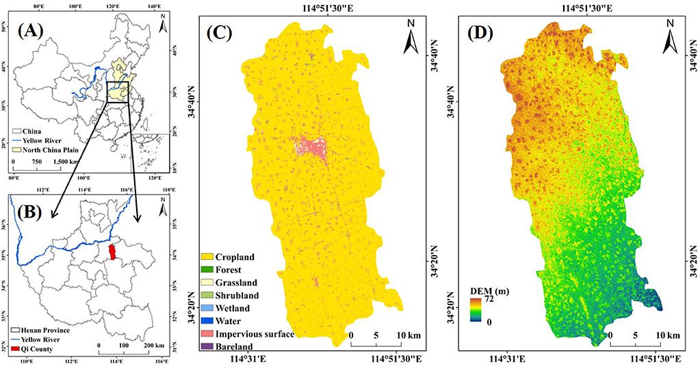
Figure 2. (A) The location of Qi County in China, (B) Enlarged map showing Qi County, Henan Province (C) Spatial pattern of the land cover types, and (D) Digital Elevation Model (DEM).

Datasets and preprocessing

Sentinel-1 images

The European Space Agency (ESA) S1 is a SAR system composed of S1A and S1B satellites, which were launched in April 2014 and April 2016, respectively. They are available at https://sentinel.esa.int/. We selected data from the interferometric wide swath (IW) mode, which is the default operational mode over land. The IW mode is in the dual polarization of vertically transmitted and horizontally received (VH) and vertically transmitted and vertically received (VV) polarizations with a temporal resolution of 12 days and a spatial resolution of 5 × 20 m (Torres et al., 2012). From October 1, 2019, to July 1, 2020, 30 S1 images as Level-1 ground range detected (GRD) were collected (Figure 3A), corresponding to “COPERNICUS/S1_GRD” of the Google Earth Engine (GEE) cloud platform.

FIGURE 3

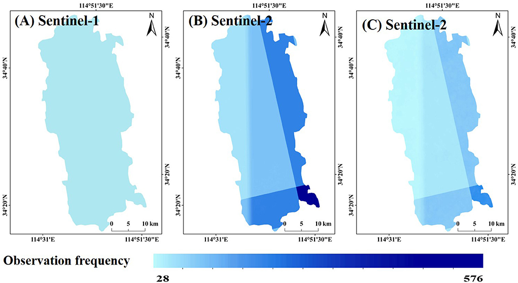
Figure 3. Numbers of observations for individual pixels during the study period. (A,B) The spatial distributions of total observations for individual pixels for S1 and S2. (C) The spatial distributions of good-quality observations for individual pixels for S2.

Some preprocessing algorithms were applied to S1 images, including orbital file correction, GRD border and thermal noise removal, radiometric calibration, and terrain correction. First, the orbit file was used to provide accurate satellite positions for each scene. Second, GRD border and thermal noise removal were applied to each scene to remove the additional noise and reduce the discontinuity in the subsamples of each scene. Third, the digital pixel value was transformed into a SAR backscattering coefficient by radiometric calibration. Finally, terrain correction was performed for each scene to correct the geometric distortion caused by the side view geometry of the acquisition system, after which shortened mask correction was performed.

Sentinel-2 images

S2 Multi-Spectral Instrument (MSI) data includes S2A and S2B images provided by the European Space Agency (ESA), and the revisit cycle of the two satellites is 5 days (Drusch et al., 2012). Because top of atmosphere (TOA) data is sensitive to changes in atmospheric composition over time, surface reflection (SR) data was selected (Jin et al., 2019). Red, near-infrared (NIR), and blue bands with a spatial resolution of 10 m and red edge (RE) bands with a spatial resolution of 20 m were used. The RE bands were resampled to 10 m by bicubic resampling to match other bands. From October 1, 2019, to July 1, 2020, 576 S2 images were collected, corresponding to “COPERNICUS/S2_SR” on the GEE cloud platform.

The quality of S2 data was assessed by the quality assessment band (QA60) in the metadata, which identifies the clouds and cloud shadows in the image as bad-quality observations and stored them as NODATA in the image (Wang et al., 2020). Specifically, since dense clouds have a high reflectance in the blue spectral region (B2), the method used to identify dense cloud pixels is based on the B2 reflectance threshold (SWIR reflectance in B11 and B12 are also used to avoid snow/cloud confusion). B10 corresponds to a high atmospheric absorption band, which means only high-altitude clouds can be detected. Additionally, since cirrus clouds are semi-transparent, they cannot be detected in the B2 blue band. Therefore, a pixel with low reflectance in the B2 band and high reflectance in the B10 band has a good probability of being cirrus cloud (a filter using morphology-based operations is also applied on both dense and cirrus masks performing). After preprocessing the image in the above steps, the total observations and good-quality observations of individual pixels were calculated, respectively (Figures 3B,C).

Ground reference data

The ground reference data of different crop types are critical to verify the crop classification algorithm. Ground reference data was collected considering the following three aspects. First, based on the Google Earth image, the stratified random sampling method was used to collect ground training and validation samples. Google Earth images with 1-m spatial resolution clearly show different ground feature types, such as the garlic field, winter wheat field, bare land. Second, two investigation routes were designed, and fieldwork was conducted to collect geo-referenced field photos from March to June 2020. These field photos include different crop types such as garlic, winter wheat, and peanuts. Third, during the fieldwork, multiple multispectral images were obtained through UAV. The spatial resolution of these multispectral images is as high as 0.1 m, which facilitates the identification of garlic among other crop types. Through the images obtained considering the above three aspects, 412 garlic samples, 451 non-garlic winter crop samples, and 453 non-winter crop samples were collected, and their spatial distribution is shown in Figure 4.

FIGURE 4

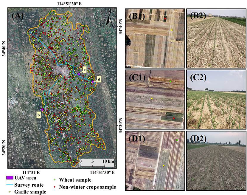
Figure 4. (A) Distribution of validation samples, including garlic, wheat, and non-winter crops. (B1–D1) Are the UAV images. (B2–D2) Are the ground observations from the field camera photograph. (B1,B2), (C1,C2), and (D1,D2) correspond to b, c, d in (A), respectively.

Land cover data

Cropland data from the FROM-GLC10 land cover product were used to mask all S2 datasets to delimit the cropland extent (Chen et al., 2019). This product was generated by RF based on S2 images and reported the cropland in 2017 with a 10-m spatial resolution. The map can be freely accessed at http://data.ess.tsinghua.edu.cn (last accessed December 15, 2021).

Methods

Figure 5 shows the algorithm framework for producing the 2020 garlic distribution map. Generally, the garlic is extracted in two steps: (1) extraction of winter crops, which is the basis for identifying the garlic, and (2) identification of the garlic within the winter crop map. Specifically, we determined the winter crop field by monitoring phenological indices of winter crops recorded in the normalized difference vegetation index (NDVI) time series. Then, based on winter crop pixels, we mapped the garlic using time series from S2 and S1. Finally, we evaluated the performance of using optical images only and coupling optical images to SAR images in mapping the garlic.

FIGURE 5

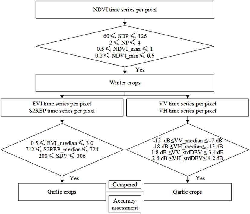
Figure 5. The algorithm framework for identifying garlic.

Index calculation

Spectral indices that are sensitive to vegetation greenness can be used to capture the physical differences of different land cover types (Di Vittorio and Georgakakos, 2018) and characterize the growth curves of different crop types (Wardlow et al., 2007). NDVI (Tucker, 1979) and enhanced vegetation index (EVI) (Huete et al., 2002), which are highly related to leaf area index and chlorophyll in the canopy, are widely used in the remote sensing inversion of vegetation phenology. Sentinel-2 red-edge position index (S2REP) (Frampton et al., 2013) can effectively monitor the growth stages of vegetation (Forkuor et al., 2018) and shows higher performance in crop classification (Yi et al., 2020). The calculation formulas are as follows:

$\begin{array}{lll}\text{NDVI}& =& \frac{{\text{ρ}}_{\text{nir}}-{\text{ρ}}_{\text{red}}}{{\text{ρ}}_{\text{nir}}+{\text{ρ}}_{\text{red}}}\\ \text{ EVI}& =& 2.5\times \frac{{\text{ρ}}_{\text{nir}}-{\text{ρ}}_{\text{red}}}{{\text{ρ}}_{\text{nir}}+6.0{\text{ρ}}_{\text{red}}-7.5{\text{ρ}}_{\text{blue}}+1}\\ \text{S}2\text{REP}& =& 705+35\times \frac{0.5\times ({\text{ρ}}_{\text{re}3}+{\text{ρ}}_{\text{red}})-{\text{ρ}}_{\text{re}1}}{{\text{ρ}}_{\text{re}2}-{\text{ρ}}_{\text{re}1}}\end{array}$

where the ρ_nir, ρ_red, and ρ_blue represent the NIR, red, and blue bands, respectively. ρ_re1, ρ_re2, and ρ_re3 represent the RE1, RE2, and RE3 bands, respectively.

Time-series construction

Compositing images at regular intervals can reduce the impact of clouds and uneven observations in time (Griffiths et al., 2019). Therefore, the VIs time series were constructed at 10-day intervals. The maximum value of all good-quality observations within a 10-day period was taken as the observation value of the 10-day period. When there was no good-quality observation in a 10-day period due to clouds, cloud shadows, and snow effects, the linear interpolation method was used to fill the data gap. The interpolated data depends on good-quality observations before and after the 10-day interval. Further, VV, VH, and standard deviation time series were reconstructed at 12-day intervals. However, even after the above steps, extremely high or low outliers may still appear in the time series, which is usually caused by cloud containment, atmospheric variability, and bidirectional effects. Therefore, the Savitzky-Golay filter was used to smooth the time series with a moving window of size 9 and a filter order of 2 (Chen et al., 2018; Pan et al., 2021a).

Annual map of winter crops in 2020

Because garlic is a winter crop, winter crops were firstly extracted from the cropland. Compared with non-winter crops, the chlorophyll content of winter crops increased continuously after sowing and decreased slightly during the vernalization period (Figure 6, October 2019 to January 2020). Therefore, there was a lower peak in the NDVI time series of winter crops during this period (Figure 6). Non-winter crops were usually harvested or not sown during this period, so their NDVI was low.

FIGURE 6

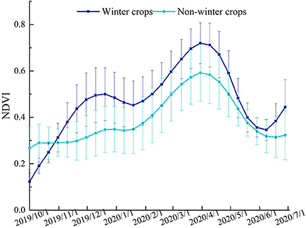
Figure 6. Temporal profile of average NDVI for winter crops and non-winter crops with standard deviation.

According to these unique phenological characteristics of winter crops, the start date of peak (SDP), the number of peaks (NP), NDVI_max, and NDVI_min phenological indices were selected. Among them, SDP is the first peak identified from October 1, 2019, to July 1, 2020; NP is the number of peaks identified from October 1, 2019, to July 1, 2020; NDVI_max is the maximum value of NDVI time series from October 1, 2019, to January 1, 2020; and NDVI_min is the minimum value of NDVI time series from June 1, 2020, to July 1, 2020.

The training samples of winter crops and non-winter crops were overlaid with the four phenology index layers to carry out a signature analysis (Figure 7). The results showed that the SDP of winter crops occurs mostly in late October to late January [day of the year (DOY) from 60 to 126]. NP is 2–4. The NDVI_max mainly gathers between 0.5 and 1, and NDVI_min mainly gathers between 0.2 and 0.6. Based on the results of signature analysis, an algorithm was developed for winter crops:

$\begin{array}{l}60\le \text{SDP }\le 126\text{ \& }2\le \text{ NP }\le 4\text{ \& }0.5\le \text{ NDVI\_max}\\ \le 1\text{ \& }0.2\le \text{ NDVI\_min }\le 0.6\end{array}$

The algorithm was applied to extract the winter crops in Qi County, and garlic mapping was performed from the winter crops.

FIGURE 7

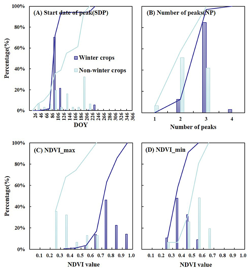
Figure 7. Signature analysis of winter crops and non-winter crops at (A) SDP, (B) NP, (C) NDVI_max, and (D) NDVI_min using the histogram statistics method.

Annual map of the garlic in 2020 based on optical images

The winter crops in Qi County were further divided into garlic and winter wheat. Although garlic and winter wheat were sown and harvested at almost the same time, the EVI and S2REP of garlic in the growth period (Figure 8, December 2019 to April 2020) were lower than those of winter wheat, and its harvest period was earlier than that of non-garlic winter crops.

FIGURE 8

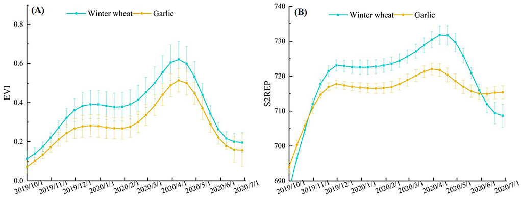
Figure 8. Temporal profile of average EVI (A) and S2REP (B) for winter wheat and garlic with standard deviation.

According to these unique characteristics of garlic, the EVI_median, S2REP_median, and start date of the valley (SDV) phenological indices were extracted. Among them, EVI_median is the median value of EVI from December 1, 2019, to April 1, 2020; S2REP_median is the median value of S2REP from December 1, 2019, to April 1, 2020; and SDV is the first valley identified from May 1, 2020, to July 1, 2020.

The training samples of garlic and winter wheat were overlaid with the three phenology index layers to carry out a signature analysis (Figure 9). The results showed that the EVI_median of garlic mainly gathers between 0.5 and 3.0, and the S2REP_median mostly gathers between 712 and 724. The SDV of garlic gathers between 200 and 306. Based on the results of signature analysis, an algorithm was developed for identifying garlic:

$\begin{array}{l}0.5\le \text{EVI\_median }\le 3.0\text{ \& }712\le \text{ S}2\text{REP\_median}\\ \le 724\text{ \& }200\le \text{ SDV }\le 306\end{array}$

The algorithm was implemented to identify garlic over the winter crops generated in section annual map of winter crops in 2020.

FIGURE 9

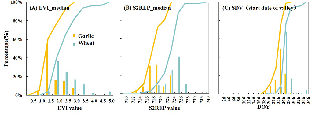
Figure 9. Signature analysis of garlic and winter wheat at (A) EVI_median, (B) S2REP_median, and (C) SDV using the histogram statistics method.

Annual map of garlic in 2020 based on SAR images

The backscattering intensities of S1 images are sensitive to crop phenology and morphological development (Mandal et al., 2020), which provides an unprecedented opportunity for garlic monitoring. Unlike winter wheat, the distance between garlic plants is larger and therefore, the backscattering coefficient of garlic is higher than that of winter wheat (Figure 10).

FIGURE 10

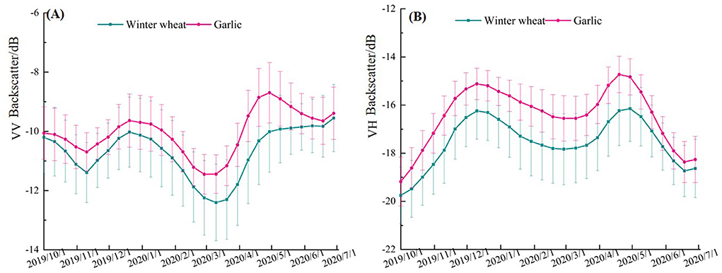
Figure 10. Temporal profile of average VV (A) and VH (B) for winter the wheat and garlic with standard deviation.

According to these unique garlic characteristics, the VV_median, VH_median, the standard deviation of VV (VV_stdDEV), and the standard deviation of VH (VH_stdDEV) phenological indices were selected to extract the garlic. Among them, VV_median and VH_ median are the median values of VV and VH from March 1, 2020, to May 31, 2020, and VH_stdDEV and VH_stdDEV are the standard deviations of VV and VH from October 1, 2019, to July 1, 2020, respectively.

The training samples of the garlic and winter wheat were overlaid with the four phenology index layers to carry out a signature analysis (Figure 11). The results showed that the VV_median of the garlic mainly gathers between −12 and −7 dB, and VH_median mostly gathers between −18 dB and −13 dB. The VV_stdDEV of the garlic mainly gathers between 1.8 and 3.4 dB, and VV_stdDEV mostly gathers between 2.6 and 4.2 dB. Based on the results of signature analysis, an algorithm was developed for identifying the garlic:

$\begin{array}{l}-12\text{ dB}\le \text{V}{\text{V}}_{-}\text{median }\le -7\text{ dB \& }-18\text{ dB}\\ \le \text{V}{\text{H}}_{-}\text{median}\le -13\text{ dB \& }1.8\text{ dB }\le \text{V}{\text{V}}_{-}\text{stdDEV}\\ \le 3.4\text{ dB \& }2.6\text{ dB }\le \text{ V}{\text{H}}_{-}\text{stdDEV}\le 4.2\text{ dB}\end{array}$

The classification algorithm was implemented to identify the garlic based on the winter crop pixels.

FIGURE 11

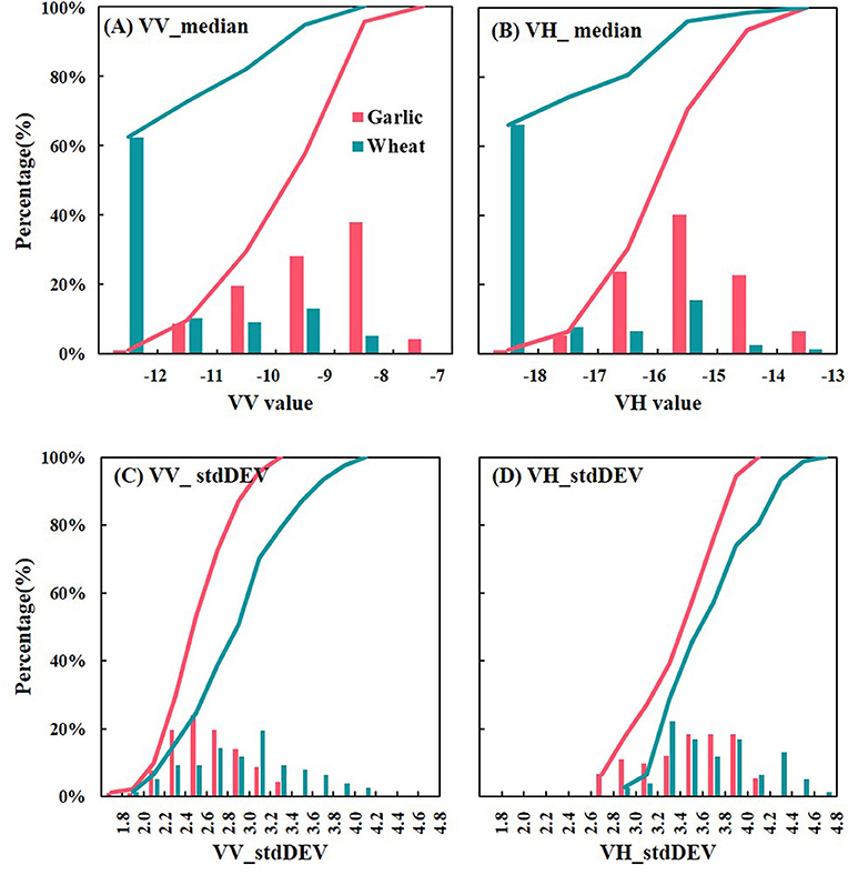
Figure 11. Signature analysis of garlic and winter wheat at (A) VV_median, (B) VH_median, (C) VV_stdDEV, and (D) VH_stdDEV using the histogram statistics method.

Accuracy assessment of the resultant annual maps

Confusion matrices were used to assess the accuracy of the winter crop and garlic distribution maps (Guo et al., 2021). It is a method to characterize the classification performance in terms of overall accuracy (OA), producer accuracy (PA), and user accuracy (UA) by constructing a matrix of classification results and sample data. It uses the following formulas,

$\begin{array}{ll}OA=\frac{T_1+T_2}{N}& (1)\end{array}$

$\begin{array}{ll}PA=\frac{T_1}{T_1+F_2}& (2)\end{array}$

$\begin{array}{ll}UA=\frac{T_1}{T_1+F_1}& (3)\end{array}$

where N is the total number of multi-classes, T₁ and T₂ are the numbers of correct classifications for class 1 and class 2, and F₁ and F₂ are the numbers of wrong classifications for class 1 and class 2, respectively. Firstly, the ground reference data obtained in section ground reference data were loaded into Google Earth, and the vector boundary of the homologous ground reference points was plotted according to the actual size and shape of the cropland. Secondly, the attributes of the vector polygons were labeled by visual interpretation and field survey data. A total of 412 garlic samples (30,658 pixels), 451 winter wheat samples (34,121 pixels), and 453 non-winter crops samples (65,112 pixels) were collected. Thirdly, these vector polygons with attribute information (e.g., the garlic, winter wheat, or non-winter crops) were converted into raster data with a spatial resolution of 10 m (Figure 12). These raster data were used as ground reference data to construct the confusion matrix with the classification results in this paper.

FIGURE 12

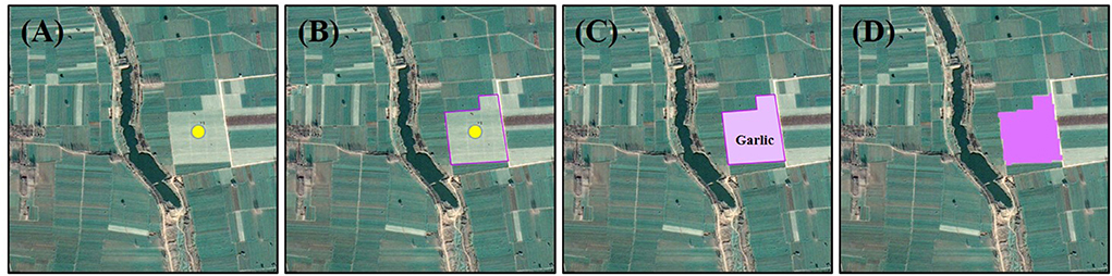
Figure 12. Flow diagram for validation data production. (A) The Google Earth image. (B) The results of vectorization, where the purple line is the garlic cropland boundary. (C) The results for identifying the attributes of the vector polygon. (D) The raster converted from the vector polygon.

Results

Annual map of winter crops in 2020

Figure 13 shows the distribution of winter crops with a 10-m resolution across Qi County in 2020. There were 1062.27 km² of winter crop fields in Qi County in 2020, accounting for 74.81% of the total cropland area. Four regions were randomly selected. In region b, the main winter crop type was winter wheat, and the main non-winter crop type was spring maize. There was a forest farm in Qi County in region c. Most cropland here was planted with trees and only a small part of the cropland was planted with garlic. In regions d and e, the main winter crop type was garlic, while spring peanuts were planted in small fields.

FIGURE 13

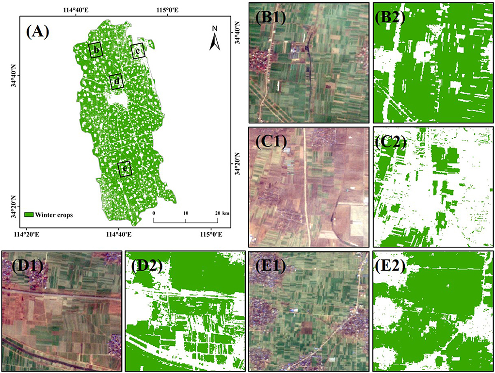
Figure 13. (A) Distribution of winter crops in Qi County in 2020. Four regions, denoted as b, c, d, and e in (A), were randomly selected. The 10-m resolution views from Sentinel-2 (December 19, 2019) are shown in (B1,C1,D1,E1), and the zoom-in views in (A) for the four regions are shown in (B2,C2,D2,E2).

Annual map of garlic in 2020

As described in sections annual map of the garlic in 2020 based on optical images and annual map of garlic in 2020 based on SAR images, the distribution of garlic in 2020 was identified by analyzing phenological indices from October 2019 to October 2020. Annual maps of garlic in 2020 with a 10-m resolution were produced (Figure 14). As per Figures 14A,B, there were 624.95 km² and 658.98 km² of garlic fields in Qi County in 2020, which accounted for 58.83 and 62.04% of winter crop fields, respectively. Four regions were randomly selected to compare the resultant annual map obtained using the two datasets. In the garlic distribution map based on S2 (Figures 14C2,D2,E2,F2), there was a great loss of cropland boundary information, and the commission and omission of the garlic fields were more serious. In the garlic distribution map based on S1 (Figures 14C3,D3,E3,F3), the cropland boundary information was relatively complete. Small garlic fields and non-garlic crop fields in the staggered distribution zone of cropland and villages were well-identified, and the classification results were better.

FIGURE 14

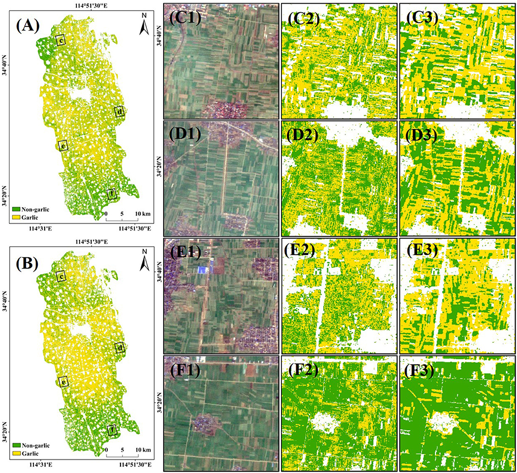
Figure 14. (A) Distribution of garlic in Qi County in 2020 only based on S2. (B) Distribution of garlic in Qi County in 2020 based on S2 and S1. Four regions, denoted as c, d, e, and f in (A,B), were selected randomly. The 10-m resolution views from Sentinel-2 (December 19, 2019) are shown in (C1,D1,E1,F1), and the zoom-in views in (A,B) for the four regions are shown in (C2,D2,E2,F2,C3,D3,E3,F3).

Accuracy assessment of the resultant annual maps

Based on the raster data obtained in section accuracy assessment of the resultant annual maps, the accuracy assessment results using the confusion matrix are shown in Table 1. The OA, UA, and PA of the winter crops distribution map were 98.07, 96.02, and 99.30%, respectively. The kappa coefficient was 0.96, which indicated a strong consistency between the classification results and the ground reference data. The accuracy assessment results showed that the algorithm proposed in this study successfully extracts the winter crop pixels in Qi County in 2020, which lays a foundation for the recognition of garlic.

TABLE 1

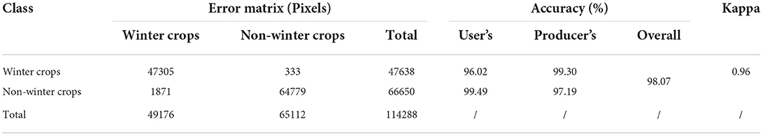
Table 1. Results of accuracy validation for the winter crops.

Furthermore, the confusion matrix was calculated using the garlic and non-garlic crop raster data obtained in section accuracy assessment of the resultant annual maps (Tables 2, 3). The OA, UA, PA, and kappa coefficient of the garlic distribution map based on S2 were 74.78%, 69.61%, 79.93%, and 0.50, respectively, while those based on S2 and S1 were 95.34%, 95.33%, 95.79%, and 0.91, respectively. Comparing the accuracy assessment results of the two algorithms, the garlic extraction algorithm based on S1 had higher accuracy and stronger consistency with the ground reference data.

TABLE 2

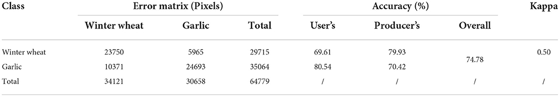
Table 2. Results of accuracy validation for the garlic crop based on Sentinel-2.

TABLE 3

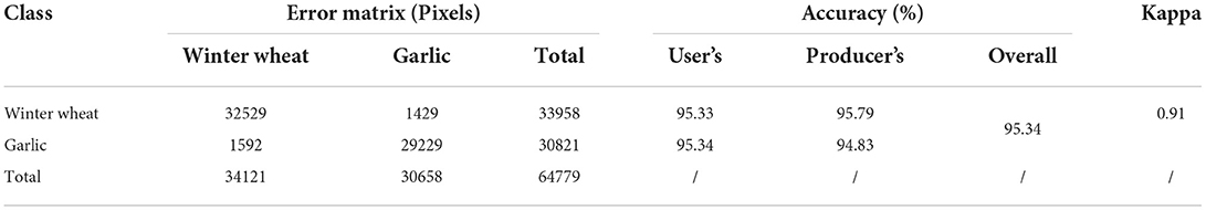
Table 3. Results of accuracy validation for the garlic crop based on Sentinel-2 and Sentinel-1.

Discussion

Integration of times series S1 and S2 images

Crops have unique spectral characteristics that make optical images an important data source for remote sensing crop recognition (Liu et al., 2017; Pan et al., 2021b). Therefore, winter crops were extracted from cropland based on S2 optical images. Compared with previous studies using MODIS images or Landsat images to extract winter crops (Pan et al., 2021b), the results provided a higher spatial resolution of 10 m. However, optical images have some limitations in distinguishing various crop types. First, the number of available optical images is often affected by clouds, cloud shadows, and snow (Ju and Roy, 2008), so good-quality images vary greatly in time and space. Although we attempted to extract the garlic using spectral differences at specific growth stages, the accuracy assessment results were not satisfactory (Table 2).

The S1 SAR images provide an opportunity to distinguish garlic from non-garlic winter crops. As shown in Figure 10, winter wheat was usually in the elongation and booting stage around April. The number and length of stems increased significantly during this period, which led to changes in the winter wheat's 3D structure. This was the main reason for the decrease in the backscattering coefficient of winter wheat (Jia et al., 2013), while garlic did not show these changes. The classification effects of various indices that have been used to develop a decision rule for classification analysis were compared, and the indices with the best separability were selected (Supplementary Figure 1). The results show that this study provides useful data for identifying garlic by remote sensing.

Algorithm development and applications

In previous studies, VIs have been used to generate garlic distribution maps (Guo et al., 2022b), but natural and human factors may lead to certain deviations in these indices. Figure 8A showed that the EVI of garlic was lower than that of winter wheat from December to April, which may be one of the indices to distinguish the garlic. However, farmers usually increase the planting density of garlic to increase the planting income, which may increase the EVI of garlic and could cause the similar EVIs of garlic and winter wheat. Although the harvest time of garlic is earlier than that of winter wheat, the 10-day resolution makes it difficult for S2 images to capture this information on a large scale. Additionally, clouds, rain, and snow may cause the fluctuation of EVI and S2REP time series, which may lead to the overlap in the VI time series of garlic and winter wheat. Therefore, it is difficult to accurately distinguish garlic and winter wheat only based on S2 data. Some studies have input the characteristics of the garlic backscattering coefficient in a specific time window into the RF classifier to extract the garlic. However, the time windows of crops with different spatial distributions vary greatly, and it is difficult to determine accurate time windows. Moreover, complex feature combinations and indices may also cause the model to overfit (Graesser and Ramankutty, 2017).

In this study, the complete growth cycle of the garlic was monitored for 1 year and several phenological indices were extracted based on the unique phenological characteristics of garlic in different growth periods. Using these phenological indices, the classification rules were established for garlic. Only pixels that meet these classification rules could be identified as garlic. Compared with other methods, the proposed algorithm simulates the growth of the garlic more realistically (Supplementary Figure 2). Furthermore, this study only took 2020 as an example of mapping the garlic distribution in Qi County. The Sentinel satellite database of the past few years is provided free of charge on the GEE cloud platform. Therefore, the algorithm can also generate garlic distribution maps from other years or regions based on these images (Supplementary Figure 3). This is because relatively consistent environmental factors such as planting mode, management mode, and climate may make garlic grow in the same cropland for many years. It is worth noting that S2 TOA data was used in the garlic distribution map in 2019 (Supplementary Figure 3), as S2 SR data for the study area over the entire 2019 were not available on the Google Earth Engine (GEE) platform. However, TOA data may lead to greater errors (Supplementary Figures 4, 5). Additionally, the algorithm proposed in this study can also generate distribution maps of other crop types by adjusting the classification indices and their threshold using local training samples.

Potential sources of uncertainty

Several factors may affect the classification results of this study. First, reliable land cover data is an important factor to improve the accuracy of the garlic distribution map. The FROM-GLC10 land cover product was used with a 10-m resolution to distinguish cropland from other land types. However, there were some classification errors in this product, especially for the staggered distribution zone of cropland and villages (Figure 12). Additionally, the product reflects the land cover in 2017, which is inconsistent with that of the study year (2020). These errors are easily propagated to the final garlic distribution map output. The publication of more reliable land cover data is expected to further improve the accuracy of the research results.

Second, for the missing values in the VI time series, linear interpolation was used based on neighboring pixels. When good-quality observations are missing at the peaks (valleys), the interpolation cannot reflect the real positions of crop growth (Guo et al., 2021). Third, in the process of extracting winter crops, the NDVI < 0.6 was used from June 2020 to July 2020 as one of the classification indices. However, there were mixed pixels of deciduous forest and winter crops on both sides of the road through fieldwork. The deciduous forest has lush branches and leaves and high chlorophyll content from June to July, which may lead to the NDVI > 0.6 of the mixed pixels. Finally, winter crops include winter wheat, winter canola, and winter vegetables, and the differences between them were not discussed in this study. A comprehensive analysis of image characteristics of different types of winter crops and improving the universality of the algorithm proposed in this study are warranted in further research.

Conclusion

In this study, an automatic mapping framework was proposed to identify and map the garlic distribution using time series optical images (Sentinel-2) and microwave images (Sentinel-1). The NDVI time series dataset was obtained from Sentinel-2 images and used to map winter crop distribution. Garlic was identified by Sentinel-2 (EVI and S2REP) and Sentinel-1 (VV, VH, and the standard deviation of VV and VH) images. Using the algorithm framework, the distribution maps of winter crops and garlic in Qi County in 2020 were generated with a 10-m resolution. The OA of the winter crop distribution map was 98.07%, with a Kappa coefficient of 0.96, laying a foundation for the recognition of garlic. The OAs of the garlic distribution map based on S2 and S1 were 74.78 and 95.34%, and the kappa coefficients were 0.50 and 0.91, respectively. The garlic distribution map obtained in this study could help stakeholders optimize the garlic planting systems for sustainable garlic production.

Data availability statement

The original contributions presented in the study are included in the article/Supplementary material, further inquiries can be directed to the corresponding author.

Author contributions

YC: data collection, writing—original draft, and writing–review and editing. YG: formal analysis, writing–original draft, and writing–review and editing. LQ: resources and validation. HX: conceptualization, resources, writing–review and editing, project administration, and funding acquisition. All authors contributed to the article and approved the submitted version.

Conflict of interest

Author YC was employed by Yankuang Donghua Construction Co., Ltd.

The remaining authors declare that the research was conducted in the absence of any commercial or financial relationships that could be construed as a potential conflict of interest.

Publisher's note

All claims expressed in this article are solely those of the authors and do not necessarily represent those of their affiliated organizations, or those of the publisher, the editors and the reviewers. Any product that may be evaluated in this article, or claim that may be made by its manufacturer, is not guaranteed or endorsed by the publisher.

Supplementary material

The Supplementary Material for this article can be found online at: https://www.frontiersin.org/articles/10.3389/fsufs.2022.1007568/full#supplementary-material

References

Agmalaro, M. A., Sitanggang, I. S., and Waskito, M. L. (2021). “Sentinel 1 classification for garlic land identification using support vector machine,” in 9th International Conference on Information and Communication Technology (ICoICT) (Yogyakarta: IEEE), 440–4. doi: 10.1109/ICoICT52021.2021.9527446

PubMed Abstract | CrossRef Full Text | Google Scholar

Amani, M., Brisco, B., Afshar, M., Mirmazloumi, S. M., Mahdavi, S., Mirzadeh, S. M. J., et al. (2019). A generalized supervised classification scheme to produce provincial wetland inventory maps: an application of Google Earth Engine for big geo data processing. Big Earth Data 3, 378–394. doi: 10.1080/20964471.2019.1690404

CrossRef Full Text | Google Scholar

Bargiel, D. (2017). A new method for crop classification combining time series of radar images and crop phenology information. Remote Sensing Environ. 198, 369–383. doi: 10.1016/j.rse.2017.06.022

CrossRef Full Text | Google Scholar

Bullock, E. L., Woodcock, C. E., and Olofsson, P. (2020). Monitoring tropical forest degradation using spectral unmixing and Landsat time series analysis. Remote Sens. Environ. 238:110968. doi: 10.1016/j.rse.2018.11.011

CrossRef Full Text | Google Scholar

Cai, Y., Li, X., Zhang, M., and Lin, H. (2020). Mapping wetland using the object-based stacked generalization method based on multi-temporal optical and SAR data. Int. J. Appl. Earth Observ. Geoinform. 92, 102164. doi: 10.1016/j.jag.2020.102164

CrossRef Full Text | Google Scholar

Chauhan, S., Darvishzadeh, R., Lu, Y., Boschetti, M., and Nelson, A. (2020). Understanding wheat lodging using multi-temporal Sentinel-1 and Sentinel-2 data. Remote Sens. Environ. 243:111804. doi: 10.1016/j.rse.2020.111804

CrossRef Full Text | Google Scholar

Chen, B., Xu, B., Zhu, Z., Yuan, C., Suen, H. P., Guo, J., et al. (2019). Stable classification with limited sample: transferring a 30-m resolution sample set collected in 2015 to mapping 10-m resolution global land cover in 2017. Sci. Bull. 64, 370–373. doi: 10.1016/j.scib.2019.03.002

CrossRef Full Text | Google Scholar

Chen, Y., Lu, D., Moran, E., Batistella, M., Dutra, L. V., Sanches, I. D. A., et al. (2018). Mapping croplands, cropping patterns, and crop types using MODIS time-series data. Int. J. Appl. Earth Observ. Geoinform. 69, 133–147. doi: 10.1016/j.jag.2018.03.005

CrossRef Full Text | Google Scholar

Di Vittorio, C. A., and Georgakakos, A. P. (2018). Land cover classification and wetland inundation mapping using MODIS. Remote Sens. Environ. 204, 1–17. doi: 10.1016/j.rse.2017.11.001

CrossRef Full Text | Google Scholar

Di, W., Lee, K., Chen, Z., Na, S., Park, C., and So, K. (2018). Design of the spatial sampling scheme for estimating the cultivation area of garlic and onion using satellite-based and unmanned aerial vehicle remotely sensed data. Korean J. Soil Sci. Fertilizer 51, 222–238. doi: 10.7745/KJSSF.2018.51.3.222

CrossRef Full Text | Google Scholar

Drusch, M., Del Bello, U., Carlier, S., Colin, O., Fernandez, V., Gascon, F., et al. (2012). Sentinel-2: ESA's optical high-resolution mission for GMES operational services. Remote Sens. Environ. 120, 25–36. doi: 10.1016/j.rse.2011.11.026

CrossRef Full Text | Google Scholar

Du, P., Samat, A., Waske, B., Liu, S., and Li, Z. (2015). Random forest and rotation forest for fully polarized SAR image classification using polarimetric and spatial features. ISPRS J. Photogrammetry Remote Sensing 105, 38–53. doi: 10.1016/j.isprsjprs.2015.03.002

CrossRef Full Text | Google Scholar

FAOSTAT, R. (2020). FAOSTAT Database. Food Agric. Organ. UN.

Google Scholar

Forkuor, G., Dimobe, K., Serme, I., and Tondoh, J. E. (2018). Landsat-8 vs. Sentinel-2: examining the added value of sentinel-2's red-edge bands to land-use and land-cover mapping in Burkina Faso. GIScience Remote Sens. 55, 331–354. doi: 10.1080/15481603.2017.1370169

CrossRef Full Text | Google Scholar

Frampton, W. J., Dash, J., Watmough, G., and Milton, E. J. (2013). Evaluating the capabilities of Sentinel-2 for quantitative estimation of biophysical variables in vegetation. ISPRS J. Photogr. Remote Sens. 82, 83–92. doi: 10.1016/j.isprsjprs.2013.04.007

CrossRef Full Text | Google Scholar

Graesser, J., and Ramankutty, N. (2017). Detection of cropland field parcels from Landsat imagery. Remote Sens. Environ. 201, 165–180. doi: 10.1016/j.rse.2017.08.027

CrossRef Full Text | Google Scholar

Griffiths, P., Nendel, C., and Hostert, P. (2019). Intra-annual reflectance composites from sentinel-2 and landsat for national-scale crop and land cover mapping. Remote Sens. Environ. 220, 135–151. doi: 10.1016/j.rse.2018.10.031

CrossRef Full Text | Google Scholar

Guo, Y., Xia, H., Pan, L., Zhao, X., and Li, R. (2022a). Mapping the northern limit of double cropping using a phenology-based algorithm and Google Earth Engine. Remote Sens. 14:1004. doi: 10.3390/rs14041004

CrossRef Full Text | Google Scholar

Guo, Y., Xia, H., Pan, L., Zhao, X., Li, R., Bian, X., et al. (2021). Development of a new phenology algorithm for fine mapping of cropping intensity in complex planting areas using sentinel-2 and google earth engine. ISPRS Int. J. Geo-Informat. 10:587. doi: 10.3390/ijgi10090587

CrossRef Full Text | Google Scholar

Guo, Y., Xia, H., Zhao, X., Qiao, L., and Qin, Y. (2022b). Estimate the earliest phenophase for garlic mapping using time series landsat 8/9 images. Remote Sens. 14:4476. doi: 10.3390/rs14184476

CrossRef Full Text | Google Scholar

Huete, A., Didan, K., Miura, T., Rodriguez, E. P., Gao, X., and Ferreira, L. G. (2002). Overview of the radiometric and biophysical performance of the MODIS vegetation indices. Remote Sens. Environ. 83, 195–213. doi: 10.1016/S0034-4257(02)00096-2

CrossRef Full Text | Google Scholar

Jia, M., Tong, L., Zhang, Y., and Chen, Y. (2013). Multitemporal radar backscattering measurement of wheat fields using multifrequency (L, S, C, and X) and full-polarization. Radio Sci. 48, 471–481. doi: 10.1002/rds.20048

CrossRef Full Text | Google Scholar

Jin, Z., Azzari, G., You, C., Di Tommaso, S., Aston, S., Burke, M., et al. (2019). Smallholder maize area and yield mapping at national scales with Google Earth Engine. Remote Sens. Environ. 228, 115–128. doi: 10.1016/j.rse.2019.04.016

CrossRef Full Text | Google Scholar

Ju, J., and Roy, D. P. (2008). The availability of cloud-free Landsat ETM+ data over the conterminous United States and globally. Remote Sens. Environ. 112, 1196–1211. doi: 10.1016/j.rse.2007.08.011

CrossRef Full Text | Google Scholar

Komaraasih, R. I., Sitanggang, I. S., and Agmalaro, M. A. (2020). “Sentinel-1A image classification for identification of garlic plants using a decision tree algorithm,” in International Conference on Computer Science and Its Application in Agriculture (ICOSICA) (IEEE), 1–6. doi: 10.1109/ICOSICA49951.2020.9243177

PubMed Abstract | CrossRef Full Text | Google Scholar

Lee, K.-D., Lee, Y.-E., Park, C.-W., and Na, S.-I. (2016). A comparative study of image classification method to classify onion and garlic using Unmanned Aerial Vehicle (UAV) imagery. Korean J. Soil Sci. Fertilizer 49, 743–750. doi: 10.7745/KJSSF.2016.49.6.743

CrossRef Full Text | Google Scholar

Lee, R.-Y., Ou, D.-Y., Shiu, Y.-S., and Lei, T.-C. (2015). “Comparisons of using random forest and maximum likelihood classifiers with worldview-2 imagery for classifying crop types,” in Proceedings of the 36th Asian Conference Remote Sensing Foster (Citeseer: ACRS).

Google Scholar

Liu, B., Shen, W., Yue, Y.-,m., Li, R., Tong, Q., and Zhang, B. (2017). Combining spatial and spectral information to estimate chlorophyll contents of crop leaves with a field imaging spectroscopy system. Precision Agricul. 18, 491–506. doi: 10.1007/s11119-016-9466-5

CrossRef Full Text | Google Scholar

Liu, J., Feng, Q., Gong, J., Zhou, J., Liang, J., and Li, Y. (2018a). Winter wheat mapping using a random forest classifier combined with multi-temporal and multi-sensor data. Int. J. Digital Earth 11, 783–802. doi: 10.1080/17538947.2017.1356388

CrossRef Full Text | Google Scholar

Liu, X., Hu, G., Chen, Y., Li, X., Xu, X., Li, S., et al. (2018b). High-resolution multi-temporal mapping of global urban land using Landsat images based on the Google Earth Engine Platform. Remote Sens. Environ. 209, 227–239. doi: 10.1016/j.rse.2018.02.055

CrossRef Full Text | Google Scholar

Mandal, D., Kumar, V., Ratha, D., Dey, S., Bhattacharya, A., Lopez-Sanchez, J. M., et al. (2020). Dual polarimetric radar vegetation index for crop growth monitoring using sentinel-1 SAR data. Remote Sens. Environ. 247:111954. doi: 10.1016/j.rse.2020.111954

CrossRef Full Text | Google Scholar

Massey, R., Sankey, T. T., Congalton, R. G., Yadav, K., Thenkabail, P. S., Ozdogan, M., et al. (2017). MODIS phenology-derived, multi-year distribution of conterminous US crop types. Remote Sens. Environ. 198, 490–503. doi: 10.1016/j.rse.2017.06.033

CrossRef Full Text | Google Scholar

Oyoshi, K., Tomiyama, N., Okumura, T., Sobue, S., and Sato, J. (2016). Mapping rice-planted areas using time-series synthetic aperture radar data for the Asia-RiCE activity. Paddy Water Environ. 14, 463–472. doi: 10.1007/s10333-015-0515-x

CrossRef Full Text | Google Scholar

Pan, L., Xia, H., Yang, J., Niu, W., Wang, R., Song, H., et al. (2021a). Mapping cropping intensity in Huaihe basin using phenology algorithm, all sentinel-2 and landsat images in google earth engine. Int. J. Appl. Earth Observ. Geoinformat. 102:102376. doi: 10.1016/j.jag.2021.102376

CrossRef Full Text | Google Scholar

Pan, L., Xia, H., Zhao, X., Guo, Y., and Qin, Y. (2021b). Mapping winter crops using a phenology algorithm, time-series Sentinel-2 and Landsat-7/8 images, and Google Earth Engine. Remote Sens. 13:2510. doi: 10.3390/rs13132510

CrossRef Full Text | Google Scholar

Poortinga, A., Tenneson, K., Shapiro, A., Nquyen, Q., San Aung, K., Chishtie, F., et al. (2019). Mapping plantations in myanmar by fusing landsat-8, sentinel-2 and sentinel-1 data along with systematic error quantification. Remote Sens. 11:831. doi: 10.3390/rs11070831

CrossRef Full Text | Google Scholar

Qiu, B., Lu, D., Tang, Z., Song, D., Zeng, Y., Wang, Z., et al. (2017). Mapping cropping intensity trends in China during 1982–2013. Appl. Geogr. 79, 212–222. doi: 10.1016/j.apgeog.2017.01.001

CrossRef Full Text | Google Scholar

Qu, C., Li, P., and Zhang, C. (2021). A spectral index for winter wheat mapping using multi-temporal Landsat NDVI data of key growth stages. ISPRS J. Photogr. Remote Sens. 175, 431–447. doi: 10.1016/j.isprsjprs.2021.03.015

CrossRef Full Text | Google Scholar

Schlund, M., and Erasmi, S. (2020). Sentinel-1 time series data for monitoring the phenology of winter wheat. Remote Sens. Environ. 246:111814. doi: 10.1016/j.rse.2020.111814

PubMed Abstract | CrossRef Full Text | Google Scholar

Siyal, A. A., Dempewolf, J., and Becker-Reshef, I. (2015). Rice yield estimation using landsat ETM+ data. J. Appl. Remote Sens. 9:095986. doi: 10.1117/1.JRS.9.095986

CrossRef Full Text | Google Scholar

Song, Y., and Wang, J. (2019). Mapping winter wheat planting area and monitoring its phenology using Sentinel-1 backscatter time series. Remote Sens. 11:449. doi: 10.3390/rs11040449

CrossRef Full Text | Google Scholar

Tan, M., Robinson, G. M., Li, X., and Xin, L. (2013). Spatial and temporal variability of farm size in China in context of rapid urbanization. Chinese Geogr. Sci. 23, 607–619. doi: 10.1007/s11769-013-0610-0

CrossRef Full Text | Google Scholar

Torbick, N., Chowdhury, D., Salas, W., and Qi, J. (2017). Monitoring rice agriculture across myanmar using time series Sentinel-1 assisted by Landsat-8 and PALSAR-2. Remote Sens. 9:119. doi: 10.3390/rs9020119

CrossRef Full Text | Google Scholar

Torres, R., Snoeij, P., Geudtner, D., Bibby, D., Davidson, M., Attema, E., et al. (2012). GMES Sentinel-1 mission. Remote Sens. Environ. 120, 9–24. doi: 10.1016/j.rse.2011.05.028

CrossRef Full Text | Google Scholar

Tucker, C. J. (1979). Red and photographic infrared linear combinations for monitoring vegetation. Remote Sens. Environ. 8, 127–150. doi: 10.1016/0034-4257(79)90013-0

CrossRef Full Text | Google Scholar

Vallentin, C., Harfenmeister, K., Itzerott, S., Kleinschmit, B., Conrad, C., and Spengler, D. (2021). Suitability of satellite remote sensing data for yield estimation in northeast Germany. Precision Agricul. 23, 52–82. doi: 10.1007/s11119-021-09827-6

CrossRef Full Text | Google Scholar

Verma, A. K., Garg, P. K., and Prasad, K. H. (2017). Sugarcane crop identification from LISS IV data using ISODATA, MLC, and indices based decision tree approach. Arabian J. Geosci. 10:16. doi: 10.1007/s12517-016-2815-x

CrossRef Full Text | Google Scholar

Wang, J., Xiao, X., Liu, L., Wu, X., Qin, Y., Steiner, J. L., et al. (2020). Mapping sugarcane plantation dynamics in Guangxi, China, by time series Sentinel-1, Sentinel-2 and Landsat images. Remote Sens. Environ. 247:111951. doi: 10.1016/j.rse.2020.111951

CrossRef Full Text | Google Scholar

Wardlow, B. D., Egbert, S. L., and Kastens, J. H. (2007). Analysis of time-series MODIS 250 m vegetation index data for crop classification in the US central great plains. Remote Sens. Environ. 108, 290–310. doi: 10.1016/j.rse.2006.11.021

CrossRef Full Text | Google Scholar

Xia, H., Zhao, J., Qin, Y., Yang, J., Cui, Y., Song, H., et al. (2019). Changes in water surface area during 1989–2017 in the Huai River Basin using Landsat data and Google earth engine. Remote Sens. 11:1824. doi: 10.3390/rs11151824

CrossRef Full Text | Google Scholar

Yang, H., Pan, B., Li, N., Wang, W., Zhang, J., and Zhang, X. (2021). A systematic method for spatio-temporal phenology estimation of paddy rice using time series Sentinel-1 images. Remote Sens. Environ. 259:112394. doi: 10.1016/j.rse.2021.112394

CrossRef Full Text | Google Scholar

Yi, Z., Jia, L., and Chen, Q. (2020). Crop classification using multi-temporal Sentinel-2 data in the Shiyang River Basin of China. Remote Sens. 12:4052. doi: 10.3390/rs12244052

CrossRef Full Text | Google Scholar

You, N., and Dong, J. (2020). Examining earliest identifiable timing of crops using all available Sentinel 1/2 imagery and Google Earth Engine. ISPRS J. Photogr. Remote Sens. 161, 109–123. doi: 10.1016/j.isprsjprs.2020.01.001

CrossRef Full Text | Google Scholar

You, N., Dong, J., Huang, J., Du, G., Zhang, G., He, Y., et al. (2021). The 10-m crop type maps in Northeast China during 2017–2019. Sci. Data 8, 1–11. doi: 10.1038/s41597-021-00827-9

PubMed Abstract | CrossRef Full Text | Google Scholar

Zhang, D., Fang, S., She, B., Zhang, H., Jin, N., Xia, H., et al. (2019). Winter wheat mapping based on Sentinel-2 data in heterogeneous planting conditions. Remote Sens. 11:2647. doi: 10.3390/rs11222647

CrossRef Full Text | Google Scholar

Zhao, X., Xia, H., Liu, B., and Jiao, W. (2022). Spatiotemporal comparison of drought in shaanxi–Gansu–Ningxia from 2003 to 2020. Using Various Drought Indices in Google Earth Engine. Remote Sens. 14:1570. doi: 10.3390/rs14071570

CrossRef Full Text | Google Scholar