Global Empirical Model of Sporadic-E Occurrence Rates

Intense ionization enhancements in the Earth’s ionosphere, known as sporadic-E (${\mathrm{E}}_s$), can degrade and severely disrupt the propagation of radio signals. Although many previous studies have analyzed the characteristics and morphologies of sporadic-E, few efforts have attempted to model global ${\mathrm{E}}_s$ occurrence rates (ORs) at high time resolutions. This study develops a global empirical model of blanketing sporadic-E occurrence rates using a Karhunen–Loéve Expansion (KLE) of a global OR climatology built with Global Navigation Satellite System radio occultation (GNSS-RO) and ionosonde observations. Using an fbE $\ge$ threshold of 3 MHz, the model outputs a blanketing sporadic-E OR for a given geomagnetic latitude, longitude, day of year, and local solar time. The model outputs are compared to digisonde observations at four sites with varying geomagnetic latitudes, resulting in correlation coefficients ranging from 0.5 to 0.9 for monthly averaged observations and an uncertainty of 11%. Furthermore, the average uncertainty is estimated to be 12%. This Global Empirical Model of Sporadic-E Occurrence Rates (GEMSOR) is capable of providing blanketing sporadic-E OR estimates for global radio frequency (RF) operations.

1 Introduction

Elevated metallic ion concentrations in the E-region of the ionosphere, known as sporadic-E (${\mathrm{E}}_s$), can significantly impact skywave radio propagation by acting as a mirror to high-frequency [HF; McNamara (1991)] and, occasionally, very-high-frequency (VHF) signals, such as amateur radio (Neubeck, 1996) and long-distance shipping information links (Chartier et al., 2022). These vertically thin layers can also severely perturb Global Navigation Satellite System (GNSS) signals (Zeng and Sokolovskiy, 2010), which can cause low-Earth orbit (LEO) position and timing disruptions from ${\mathrm{E}}_s$-induced scintillation (Kintner et al., 2007; Yue et al., 2016). Furthermore, over-the-horizon radar (OTHR), which uses HF signals and can provide detection ranges over thousands of miles, is of special interest to the aviation industry and military applications (Headrick et al., 2008) but is extremely susceptible to ${\mathrm{E}}_s$ impacts (Thayaparan and MacDougall, 2005; Cameron et al., 2022). For these reasons, estimates of sporadic-E occurrence can provide valuable information to technological efforts relying on skywave or trans-ionospheric radio wave propagation.

Sporadic-E is generally agreed to be caused by persistent metallic ions in the E-region of the ionosphere, and these ions are acted upon by forces caused by wind shears, tides, and gravity waves in mid-latitude regions, electromagnetic field (gradient) instabilities at equatorial regions, and high-energy particles driven by convection electric fields at high latitudes and poles (Whitehead, 1989; Mathews, 1998; Haldoupis et al., 2007). These forces result in the formation of ${\mathrm{E}}_s$ layers that can range in size from kilometers to several hundred kilometers, in distinct layers 6–10 km apart, at altitudes of 90–120 km, with lifetimes in the order of hours (Cathey, 1969; Whitehead, 1989; MacDougall et al., 2000; Chu et al., 2014; Maeda and Heki, 2015).

While many techniques have been used to monitor sporadic-E, including incoherent scatter radars (ISRs) (Mathews (1998); Hysell et al. (2009)), Super Dual Auroral Radar Network (SuperDARN) (Kunduri et al. (2023)), and long-wavelength arrays (LWAs) (Obenberger et al. (2021)), global ${\mathrm{E}}_s$ coverage requires a large number of observations spread throughout the globe. Currently, global ${\mathrm{E}}_s$ observations are provided by ionosondes (Smith, 1957; Merriman et al., 2021) or GNSS radio occultation (RO) (Wu et al. (2005); Chu et al. (2014); Arras and Wickert (2018); Niu et al. (2019); Yu et al. (2020). Ground-based GNSS receivers have also been used to monitor ${\mathrm{E}}_s$ (Maeda and Heki, 2015; Sun et al., 2021), but they are limited to intense layers with critical sporadic-E frequencies, foEs, greater than $\sim$16 MHz, while the unique geometry of GNSS-RO observations allows for strong perturbations by the vertically thin ${\mathrm{E}}_s$ layers (Wu et al., 2005; Zeng and Sokolovskiy, 2010; Emmons et al., 2022). While ionosondes provide a direct measurement of sporadic-E layers (Reddy and Mukunda Rao, 1968), the integrated nature of GNSS-RO observations produces ambiguities in the measurements, which have produced substantial discrepancies between ${\mathrm{E}}_s$ parameter estimates (Emmons et al., 2023) and occurrence rates (Carmona et al., 2022).

Taking into account these observational challenges, many studies have largely focused on examining ionosphere climatology using GNSS-RO and/or ionosonde data, with many focusing on describing the ${\mathrm{E}}_s$ intensity or occurrence rate (OR) (Niu et al., 2019; Yu et al., 2020; Gooch et al., 2020; Merriman et al., 2021; Ellis et al., 2024). Several studies have developed morphologies or climatologies of sporadic-E ORs, but limited data density generally results in a trade-off between high spatial or high temporal resolution (Smith, 1957; Arras and Wickert, 2018; Arras et al., 2022a; Hodos et al., 2022). Recently, global models for determining the intensity of sporadic-E have been created from GNSS-RO observations using the maximum amplitude scintillation index, ${\mathrm{S}}_4$-max, as a proxy for the sporadic-E intensity (Yu et al., 2022; Tian et al., 2023). The relatively large GNSS-RO data density over space and time allows the intensity models to perform spatiotemporal fits or training directly on the RO dataset.

In contrast, for OR models, the overall spatiotemporal data density is drastically reduced via the requirement to calculate ORs using a sufficiently large number of data points within a bin. For example, Hodos et al. (2022) developed OR climatology from ionosonde and GNSS-RO observations that required at least 25 measurements within a spatiotemporal bin to cap the standard error at 10%, which limited the final climatology to monthly 5°$\times$5° latitude–longitude or seasonal 12-min$\times$5° time-latitude bins. This reduction in temporal resolution does not allow for direct fitting or training of spatiotemporal data, as performed for the ${\mathrm{E}}_s$ intensity models. While ionosonde-based OR climatologies have the potential to investigate shorter temporal scales due to the regular $\sim$15-min sounding cadence, the large spatial gaps between ionosonde sites cause large uncertainties in OR estimates between sites (Smith, 1957; Merriman et al., 2021).

However, considering the practical implications of blanketing ${\mathrm{E}}_s$ occurrences, there is a clear interest in providing an empirical model of ${\mathrm{E}}_s$ ORs with high spatiotemporal fidelity and confidence, which is the goal of the proposed Global Empirical Model of Sporadic-E Occurrence Rates (GEMSOR) model. While the model developed by Hodos et al. (2022) provided global spatial and temporal trends of sporadic-E occurrence, the coarse time resolution makes the dataset impractical as a model. To develop a practical model with appropriate time resolution, GEMSOR uses a Karhunen–Loéve Expansion (KLE) of the climatology developed by Hodos et al. (2022) with interpolation between monthly OR maps. This interpolation drastically improves the temporal resolution from monthly to hourly, thereby providing a global empirical model of blanketing sporadic-E ORs for fbEs $\ge$ 3.0 MHz as a function of geomagnetic latitude, geographic longitude, day of year, and local solar time. Details of the model development are outlined below, along with the results of a validation effort using ionosonde observations from four sites with varying geomagnetic latitudes.

2 Materials and methods

2.1 Dataset development

Hodos et al. (2022) created global maps of ${\mathrm{E}}_s$ ORs using two different GNSS-RO techniques and ionosonde soundings from data covering 2006–2019, resulting in global ORs for fbEs $\ge$ 3 MHz and fbEs without an intensity threshold. They produced monthly global maps of fbEs ORs binned in 5° geomagnetic latitude $\times$ 5° geographic longitude intervals, as well as seasonal maps binned in 5° geomagnetic latitude $\times$ 12-min bins. The current study only examined the occurrence rates of fbEs $\ge$ 3.0 MHz (moderate fbEs) by using the monthly results obtained by Hodos et al. (2022) by the application of the RO-based ${\mathrm{E}}_s$ detection technique developed by Chu et al. (2014) and further adjusted by Carmona et al. (2022). Two additional modifications to the analysis conducted by Hodos et al. (2022) were implemented. First, this study only sought to model global moderate-fbEs ORs during geomagnetic quiet conditions, defined as a planetary K (Kp) index $\le$ 4 and an Auroral Electrojet (AE) index $<$ 500 nT, in contrast to 200 nT used by Hodos et al. (2022). This was found to be in agreement with the observations of Kamide and Akasofu (1983) and simultaneously increased the number of usable observations from 4,595,998 to 10,101,710. Second, the temporal binning of the 5°$\times$12-min data was increased to 1 h. This increase resulted in the development of a more manageable model by reducing the temporal space being modeled as well as increasing the observations in each spatiotemporal bin on average.

These observations are displayed in Figure 1, and we can see that the GNSS-RO observations vary more significantly over geomagnetic latitude than longitude or local solar time. The large number of digisonde observations is also apparent and results in pronounced banding in the spatiotemporal data.

Figure 1

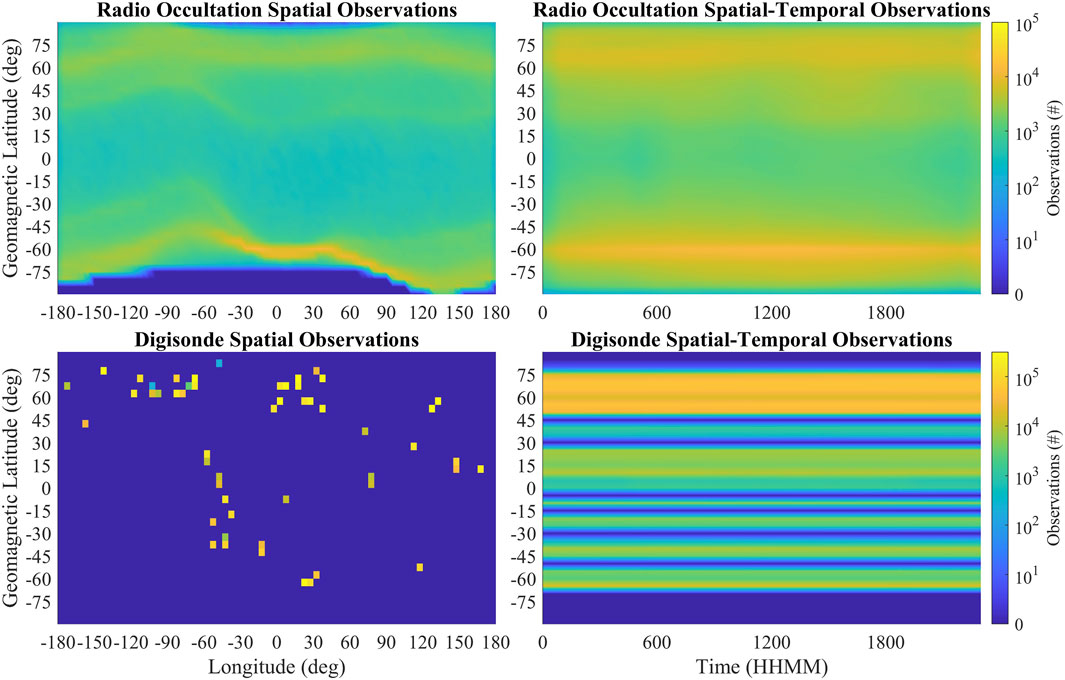
Figure 1. Top left: total observation count for GNSS-RO spatial measurements. Top right: total observation count for GNSS-RO spatiotemporal measurements. Bottom left: total observation count for digisonde spatial measurements. Bottom right: total observation count for digisonde spatiotemporal measurements. GPS-RO observations provide greater global coverage with lower data density than digisonde observations that provide higher data density at the cost of global coverage.

The presented model was developed using geomagnetic latitude and is defined as the dip angle or magnetic field inclination at an altitude of 100 km, as established by the World Magnetic Model (WMM). The average inclination from the 2010 WMM epoch was used for climatology and model development (Maus et al., 2010).

As described by Hodos et al. (2022), the sparsity of the COSMIC dataset and the requirement of at least 25 observations per bin result in a spatial resolution limited to 5° latitude $\times$ 5° longitude. Bins that do not satisfy this minimum observation count do not have a calculated OR and are consequently set to 0. This ensures there are no gaps in the data prior to model development. This spatial resolution resulted in global fbEs OR maps for each month of the calendar year with an average of 85$\%$ of spatial bins $(\sim 2296/2701)$ having a calculable OR throughout the year. More than half (56$\%$) of the insufficient-observation bins were located beyond 75°N or 75°S. Most of the remaining low-observation bins were located between 30°N and 30°S and 0$°$ E and 150$°$ E. These spatially binned monthly data are called spatial data.

This study chose to integrate data over longitude in order to increase the temporal resolution, allowing the development of monthly fbEs OR maps with a spatial resolution of 5$°$ geomagnetic latitude and a temporal resolution of 1 h. These data are called spatiotemporal data, with an average of 97$\%$ of the spatiotemporal bins $(\sim 861/888)$ containing a calculable fbEs OR, with 100$\%$ of these being between 75$°$ N and 75$°$ S.

To reduce the discontinuities resulting from the incorporation of irregularly spaced ionosonde sites combined with asymmetric spatial observation densities (Figure 1), both data sets were filtered using a 2D Gaussian smoothing kernel. This has the added benefit of adjusting bins that were previously set to 0 due to insufficient observations to a value dependent on its neighboring bins. Calculating the average difference between the original climatology and the Gaussian-filtered climatology on a monthly basis and averaging over a year yielded an OR mean absolute difference of 2$\%$ for both the spatial and spatiotemporal data.

2.2 Model development

Karhunen–Loéve Expansion (KLE) has many different names, including principal component analysis (PCA), proper orthogonal decomposition (POD), and empirical orthogonal functions (EOFs) (Kirby, 2000; Björnsson and Venegas, 1997). The terminology of KLE is used throughout this report because it was used in the primary reference, Kirby (2000). KLE allows recasting each dataset as a combination of coefficients and modes: $X=\mathrm{\Psi }A$, where $X$ is an $N\times P$ data matrix with $N$ discrete data positions and $P$ steps in time (Kirby, 2000). This matrix has also been mean subtracted over time $(P)$. In the spatial case, $X$ is labeled $X^{\varphi \theta }$ and consists of 12 column vectors, one for each month, with each element of the vector representing the occurrence rate for a distinct spatial bin. The combination of geomagnetic latitude, $\varphi$, and geographic longitude, $\theta$, results in a (37$\cdot$73)$\times$12 or $2701\times 12$ matrix. In the spatiotemporal case, $X$ is labeled $X^{\varphi t}$ and consists similarly of 12 column vectors, with each element pertaining to a discrete spatiotemporal bin, i.e., each combination of geomagnetic latitude, $\varphi$, and hourly local solar time $t$. In simpler terms, the monthly global maps have been converted to arrays representing each month and ordered chronologically for both the spatial and spatiotemporal cases.

$\mathrm{\Psi }$ is an $N\times N$ matrix of column-wise eigenvectors of the covariance matrix and will be referred to as the modes. $A$ is an $N\times P$ matrix of expansion coefficients, and both of these matrices are shown in Figures 3, 4. The eigenvalues, ${\lambda }_i$, of the spatial covariance matrix and their corresponding modes are ordered from the largest, ${\lambda }_1,{\psi }_1$, to the smallest, ${\lambda }_N,{\psi }_N$, as larger eigenvectors explain a greater amount of variance in the data (Björnsson and Venegas, 1997). Using the sum of all the eigenvalues to produce normalized eigenvalues, ${\widehat{\lambda }}_i$, after normalizing, the spatial and spatiotemporal eigenvalues are quite similar, as shown in Figure 2. Both only require two modes to explain $\sim 90\%$ of the variance.

Figure 2

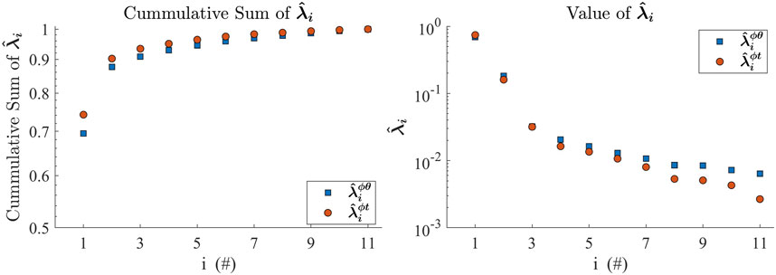
Figure 2. Left: cumulative sum of the normalized eigenvalues from largest to smallest for both the spatial and spatiotemporal data. Right: value of each normalized eigenvalue from largest to smallest for both the spatial and spatiotemporal data. Each dataset only requires two modes to explain $\sim$90% of the variance.

Typically, only the larger eigenvalues and modes more easily associated with a physically describable phenomenon are used for further analysis (Björnsson and Venegas, 1997). However, this study used all 11 nonzero modes for two reasons. First, only the largest eigenvalues are usually selected to reduce the impact of noise in the analysis, but this was addressed previously using the Gaussian filter. Second, limiting the number of modes will increase the uncertainty in the final outputs. Without the Gaussian filter, the primary modes associated with the largest eigenvalues retained much of the small-scale variation, which did not produce a smooth empirical model as desired. Therefore, the Gaussian filter was applied before KLE, and all 11 modes were retained to reduce uncertainties.

With the modes, columns of $\mathrm{\Psi }$, and expansion coefficients $A$ determined, the smoothed data, $X$, can be recast as an expansion shown in Equation 1

$OR\left(m,x_j\right)={\displaystyle \sum _{i=1}^r}{\alpha }_i\left(m\right){\psi }_i\left(x_j\right),(1)$

where $OR$ is the occurrence rate, $m$ is the calendar month, $x_j$ is the discrete spatial, $(\varphi ,\theta )$, or spatiotemporal, $(\varphi ,t)$, position, $r$ is the rank of $X$, ${\alpha }_i$ is the $i$th row vector of $A$, and ${\psi }_i$ is the $i$th column vector of $\mathrm{\Psi }$ (Kirby, 2000). Each coefficient, ${\alpha }_1$ through ${\alpha }_N$, was treated as a function of time $(m)$, with $P$ discrete steps in time. This was exploited to generate climatologies for each day.

The three largest coefficients and their corresponding modes are shown in Figure 3 for the spatial data and in Figure 4 for the spatiotemporal data. The modes were transformed into their two-dimensional representation prior to plotting. Figures 3, 4 show that mode and coefficient 1 for both the spatial and spatiotemporal analyses capture the well-documented seasonal variation that peaks in the boreal summer and winter months (Whitehead, 1989; Haldoupis et al., 2007). Mode and coefficient 2 highlight seasonal peaks in the spring and fall. Mode and coefficient 3 highlight particularly high-variance regions when analyzing the spatial domain and particularly high-variance latitude bands and times of day when analyzing the spatiotemporal domain.

Figure 3

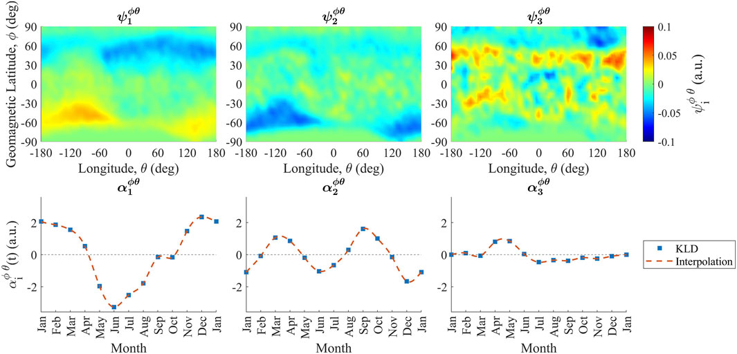
Figure 3. Top panel: eigenvectors as determined by the KLE when applied to the spatial data. Bottom panel: coefficients as determined by the KLE when applied to the spatial data. Regions of larger variance in the Northern and Southern Hemisphere are seen clearly in modes 1 and 2 with the corresponding seasonal changes seen in coefficients 1 and 2, respectively.

Figure 4

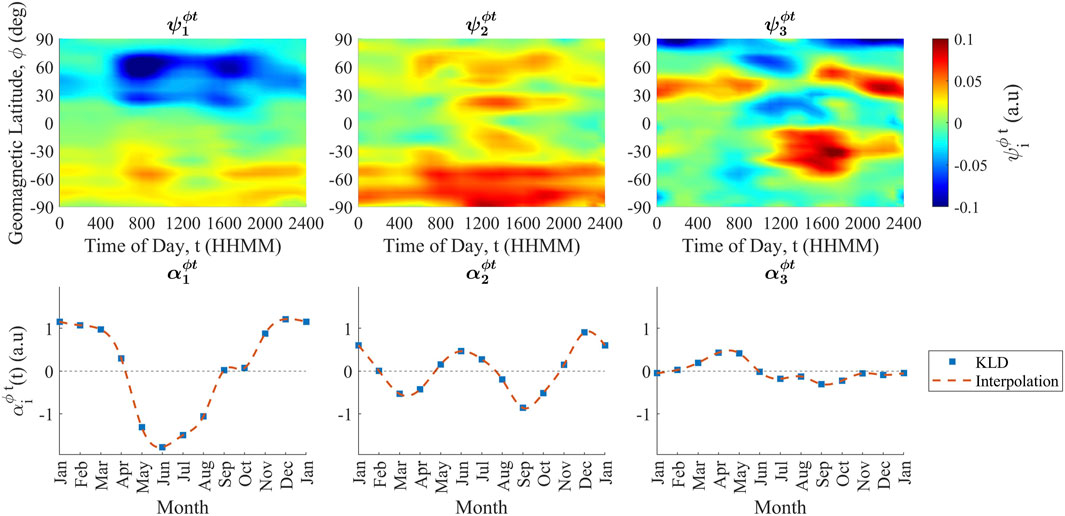
Figure 4. Top panel: eigenvectors as determined by the KLE when applied to the spatiotemporal data. Bottom panel: coefficients as determined by the KLE when applied to the spatiotemporal data. Latitudes and times of day with larger variance are seen with their corresponding changes throughout the year, as shown in the coefficients.

With the data represented in the KL basis, the coefficients, ${\alpha }_i(m)$, were interpolated over time using a cubic spline interpolation. This interpolation was performed such that the number of time steps was increased from 12 to 365, resulting in a daily time resolution as opposed to the original monthly time resolution. This spline for each coefficient, shown in Figures 3, 4, results in a new interpolated data matrix, $\tilde{X}$, that has a column for each day of the year, $d$. These columns were then converted back to matrix form. Some results for the month of June from both the spatial and spatiotemporal data are shown in Figure 5. Note that since the original data were summed over an entire month, the spline was performed so that the original data for each month (i.e., $\alpha (d)=\alpha (m)$) will appear at each month’s midpoint. From this, the daily maps over a month should approximately average out to the original monthly map. This spatiotemporal interpolation is taken over days of the year, and the local solar time is provided for a particular day of year by the interpolated spatiotemporal data (see examples in Figure 5).

Figure 5

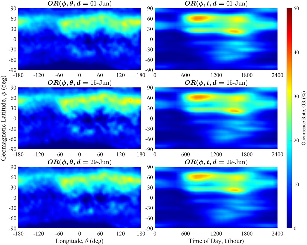
Figure 5. Top panel: results from interpolated coefficients corresponding to 1 June. Middle panel: results from interpolated coefficients corresponding to 15 June. Bottom panel: results from interpolated coefficients corresponding to 29 June. There are subtle but notable changes over time after applying the interpolated coefficients.

It is important to note that the daily spatial maps should be seen as averages for each bin over a day. After generating daily climatologies, the values were analyzed to determine whether any were nonsensical ($O{R}_i<0\%$, $O{R}_i>100\%$). There were no values generated greater than 100%, and the largest negative value was $>-0.5\%$, with 99.8% of values greater than $-1\times 10^{-8}\%$. This indicates that the majority of the negative values were due to computer precision, and the interpolation did generate plausible values. These negative values were set to 0 before the subsequent combination.

The interpolated global fbEs OR maps for every day of the year in both the spatial, $OR(\varphi ,\theta ,d)$, and spatiotemporal, $OR(\varphi ,t,d)$, representations can be combined to create a final model, $OR(\varphi ,\theta ,d,t)$. With the average occurrence rate over a given day in the spatial data, an appropriate hourly fbEs OR can be calculated using the spatiotemporal data.

The following requirements were used for this calculation. First, for an fbEs OR, $OR(\varphi ,\theta ,d,t)$, the outputs must be within the valid range of 0%–100%. Second, the predicted hourly average fbEs OR, over a given day for a specific spatial bin, should be equivalent to the calculated spatial OR for the same bin, as shown in Equation 2. This is because this model’s temporal fbEs OR output for a given geomagnetic latitude, longitude, and day should be consistent with the input spatial fbEs OR for the same location.

$\frac{{\displaystyle \sum _{t=0}^{23}}OR\left(\varphi ,\theta ,d,t\right)}{23}=OR\left(\varphi ,\theta ,d\right),(2)$

where $t$ has a range of 0–23 h in 1-h increments, resulting in 24-h fbEs ORs for each day. Third, given that the above two assumptions are satisfied, the temporal output should relatively follow the input profile. That is, the local minima and maxima during a day should remain at the same hourly position.

For clarity, the array consisting of all hourly fbEs ORs for a given $\varphi$ and $d$ of a spatiotemporal climatology is defined as

${\overrightarrow{OR}}_t\left(\varphi ,d\right)=\left[OR\left(\varphi ,t=0,d\right),OR\left(\varphi ,t=1,d\right),\dots OR\left(\varphi ,t=23,d\right)\right],(3)$

and we use the same convention for an array of final output ORs for a given day, ${\overrightarrow{OR}}_t(\varphi ,\theta ,d)$. Note that each value of $t$ indicates the entire hour period (i.e., $t=6$ indicates the local solar time of 0600–0659). Due to the first two conditions, any $OR(\varphi ,\theta ,d)=0$ results in ${\overrightarrow{OR}}_t(\varphi ,\theta ,d)=\vec{0}$. In all other cases, ${\overrightarrow{OR}}_t(\varphi ,d)$ was scaled so that it had minimum values of 0 and maximum values equal to the corresponding $OR(\varphi ,\theta ,d)$. This array is defined as

$s{\overrightarrow{OR}}_t\left(\varphi ,\theta ,d\right)=\frac{{\overrightarrow{OR}}_t\left(\varphi ,d\right)-min\left({\overrightarrow{OR}}_t\left(\varphi ,d\right)\right)}{max\left({\overrightarrow{OR}}_t\left(\varphi ,d\right)\right)-min\left({\overrightarrow{OR}}_t\left(\varphi ,d\right)\right)}\cdot OR\left(\varphi ,\theta ,d\right).(4)$

Defining the mean of this array as $\beta (\varphi ,\theta ,d)$, the difference needed to adjust $s{\overrightarrow{OR}}_t(\varphi ,\theta ,d)$ so that it has an average value equal to $OR(\varphi ,\theta ,d)$ was determined. This difference is called $\mathrm{\Delta }(\varphi ,\theta ,d)=OR(\varphi ,\theta ,d)-\beta (\varphi ,\theta ,d)$. The final fbEs OR in array notation is then ${\overrightarrow{OR}}_t(\varphi ,\theta ,d)=s\overrightarrow{O{R}_t}(\varphi ,\theta ,d)+\mathrm{\Delta }(\varphi ,\theta ,d)$. In functional form, this becomes

$OR\left(\varphi ,\theta ,d,t\right)=sOR\left(\varphi ,\theta ,d,t\right)+\mathrm{\Delta }\left(\varphi ,\theta ,d\right).(5)$

Equation 4 maintains the structure of the local solar time profile, ${\overrightarrow{OR}}_t(\varphi ,d)$, and scales it to the corresponding location daily average, $OR(\varphi ,\theta ,d)$. Adding $\mathrm{\Delta }(\varphi ,\theta ,d)$, as shown in Equation 5, ensures that this local solar time profile averages to the corresponding location’s daily average, $OR(\varphi ,\theta ,d)$. This process ensures that requirements 2 and 3 are both satisfied. Satisfaction of the first requirement was verified numerically post hoc.

An example of this combination for throughout the year and at mid-latitudes is shown in Figure 6. It visually appears to satisfy all requirements and shows examples of where the scaling resulted in an increase in the hourly fbEs OR, a decrease in the hourly fbEs OR, and sometimes both. Figure 6 shows that, in the summer months, a distinct semidiurnal trend was apparent with peaks in the morning and afternoon, which is in agreement with the observations of Whitehead (1989) and Smith (1957). There was no significant increase in the model fbEs OR peak in the summer months due to the relatively small increase in the calculated spatial OR at this particular location during summer, as shown by the dotted red line. While the spatiotemporal data show larger peaks, they are integrated over longitude and may include other regions with substantially larger variation than the longitude of interest. The scaling method forced the hourly fbEs OR to average to this value over a day. Since the underlying data did not support a large average increase in the fbEs OR at this location, the model could not support it as well.

Figure 6

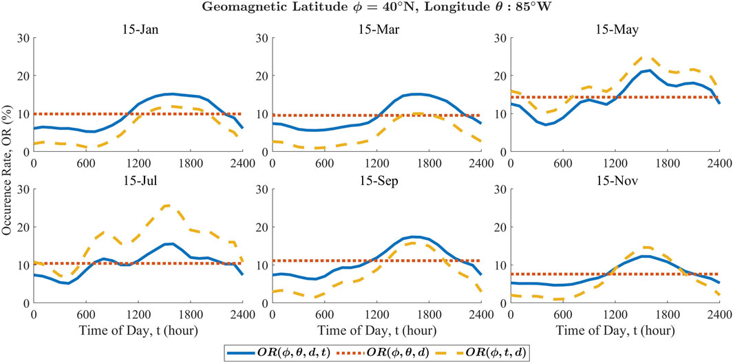
Figure 6. Results of scaling the interpolated climatologies at mid-latitudes. Blue indicates the final result, red indicates the interpolated spatial data, and yellow indicates the interpolated spatiotemporal data. The imposed requirements are seen to produce results that are sensible and consistent between datasets. Each subplot depicts a different calendar day (day of year) at the given location.

3 Results

Videos showing the final GEMSOR predictions on a global map with a time resolution of 3 h are given in Supplementary Material, and the model can be downloaded from GEMSOR-OSF. Instead of analyzing a subset of global OR maps here, we focus on uncertainties and validation.

3.1 Error analysis

Considering that each calculated fbEs OR was treated as a distribution of binary events, each bin follows a Bernoulli distribution and has a standard deviation, ${\sigma }_{B,i}$ shown in Equation 6

${\sigma }_{B,i}=\sqrt{O{R}_i\left(O{R}_i-1\right)},(6)$

where $O{R}_i$ is the calculated fbEs OR for the $i$th spatial or spatiotemporal bin, as performed by Hodos et al. (2022). Therefore, each bin has a sampling distribution with a standard error of ${\sigma }_i={\sigma }_{B,i}/\sqrt{n_i}$, where $n_i$ is the total number of observations in the $i$th bin.

Before performing the Gaussian filter, with the exception of bins that had insufficient observations for calculation, $n_i<25$, each spatial and spatiotemporal fbEs OR has an associated standard deviation, ${\sigma }_i^{\varphi \theta }$ or ${\sigma }_i^{\varphi t}$. These uncertainties are propagated through Equation 5, using the formula for the propagation of error for two variables (Ku et al., 1966). The application of the Gaussian filter resulted in a mean absolute error of ${\bar{\sigma }}^{\varphi \theta }\approx 2.3\%$ and ${\bar{\sigma }}^{\varphi t}\approx 2.0\%$ throughout the year. This was treated as a baseline error that will be added to the propagated bin uncertainty. Since all 11 nonzero modes and coefficients were used during the KLE for both data bins, this study assumes that no error was introduced during the KLE.

The propagated uncertainties were averaged over both month and hour for the entire year, and uncertainties for some months are shown in Figure 7, and the uncertainties for some selected hours are shown in Figure 8. Larger uncertainties were observed when examining the model on a monthly basis compared to an hourly basis. This was likely due to the fact that there is more variance in the fbEs OR over a month at a given location than during a given hour over a year. This is supported by the clear increase in uncertainty during seasonal peaks and local solar time peaks, as shown in Figures 7, 8. When analyzing the entire globe on a monthly basis, the uncertainty only occasionally approached 20% and was location-dependent. During the boreal spring and fall months, the uncertainty rarely exceeded 10%. Peak uncertainty is shown at (Figure 8) approximately 1600 L, with the minimum uncertainty in the late-evening and early-morning hours. However, at all times of the day, the average uncertainty remains below 10%.

Figure 7

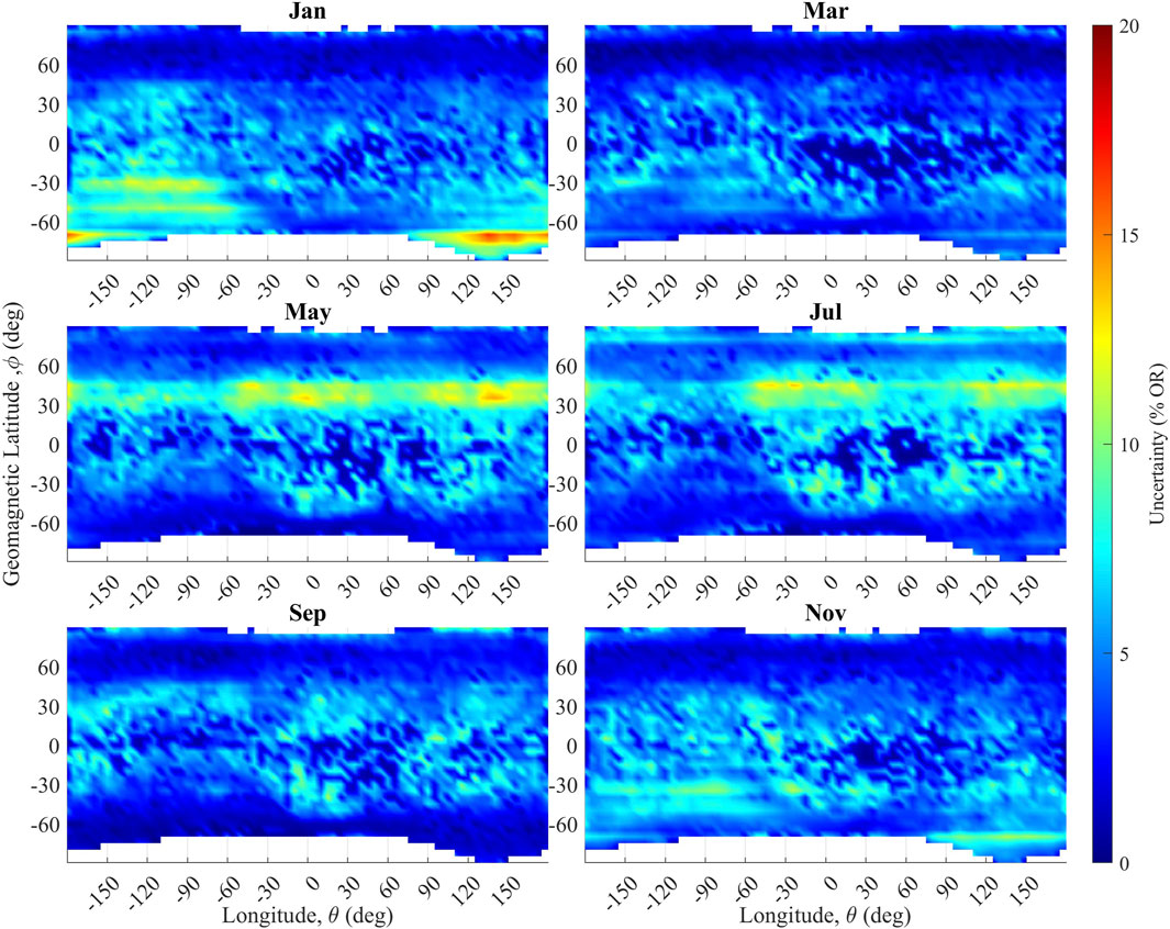
Figure 7. Average calculated uncertainty for selected months. Locations with insufficient observations are indicated by white. There is increased uncertainty at locations and times of year with higher ORs.

Figure 8

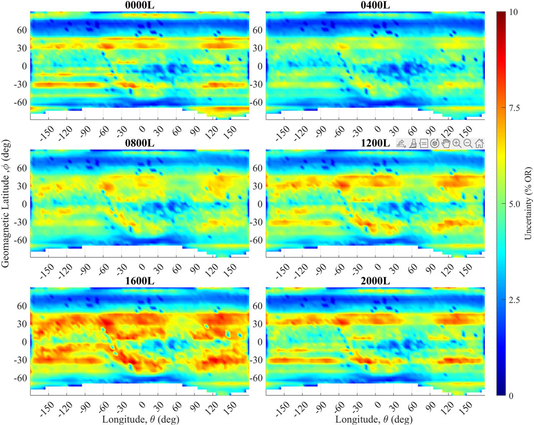
Figure 8. Average calculated uncertainty for selected hours. Note the change in scale from Figure 7. Locations with insufficient observations are indicated in white. There is increased uncertainty at times of day with higher ORs.

Since the total observation threshold was kept at 25, as outlined in Hodos et al. (2022), bins that did not have at least 25 observations had no calculated uncertainty, and their fbEs OR was set to 0% unless the Gaussian filter resulted in a weighted OR in that bin. As mentioned above, this largely affected high latitudes, in particular 75°S and below. Although this limits the use of the word global, these regions of the world are particularly impacted by auroral-E, which can be difficult to differentiate from sporadic-E (Roberts, 2024). Therefore, it may be more appropriate to develop a separate model that specifically accounts for auroral-E at these high latitudes.

Since the KLE resulted in 365 global maps of fbEs ORs and there were only measurement uncertainty values for each month, initial monthly uncertainties were used for all calculations for each month. Taking the average of all determined uncertainties results in a mean uncertainty, $\bar{\sigma }=5\%$. Furthermore, Carmona et al. (2022) found that the technique used by Chu et al. (2014) had a mean absolute error of 3$\%$ relative to ionosonde observations. This will be taken as an average global measurement error and added to the above errors, resulting in a final average error of 12$\%$.

While this error analysis considers the impacts of GNSS-RO sampling, smoothing, and combining ORs, it does not account for any uncertainty in ionosonde measurements. This analysis assumes that there are no errors associated with the ionosonde measurements, in particular, ionograms automatically scaled by ARTIST-5. Although ionosonde soundings were taken as “ground truth,” Stankov et al. (2023) showed automatically scaled foEs errors to range from $\left[-0.80,0.35\right]$ MHz compared to manually scaled ionograms. It is unclear how this foEs uncertainty relates to an fbEs OR uncertainty as presented here, and the authors are unaware of an ${\mathrm{E}}_s$ OR error study for automatically scaled ionograms. For these reasons, it is assumed that the ionosonde ${\mathrm{E}}_s$ measurements have no error as quantifying any such error would be largely arbitrary.

3.2 Validation

Validation was performed by comparing the model’s outputs to corresponding observations collected by the Global Ionosphere Radio Observatory at four different locations: El Arenosillo, Spain (37.1°N, 6.7°W); Fortaleza, Brazil (3.9°S, 38.4°W); Gakona, Alaska (62.38°N, 145.0°W); and Hermanus, South Africa (34.42°S, 19.22°E). Note that geographic coordinates are given above. These locations were selected to sample a variety of geomagnetic latitudes and at times will be referred to by their International Union of Radio Science (URSI) station codes: EA036, FZA0M, GA762, and HE13N, respectively. El Arenosillo was chosen to evaluate the performance in the Northern Hemisphere at geomagnetic mid-latitudes. Hermanus was chosen for Southern Hemisphere mid-latitudes, Gakona, for high latitudes, and Fortaleza, for low latitudes. Data from 2020–2022 were used, totaling 512,031 observations, and the average geomagnetic inclination from WMM 2020 at each location over the 3-year period was used as the geomagnetic latitude (Chulliat et al., 2020).

Two types of comparison are performed: an hour-to-hour comparison and a monthly averaged comparison. Hours that had total ionosonde observations of $n_t<1$ were not used for the hourly comparison, resulting in 14%, 10%, 3%, and 19% of hour intervals being discarded for the sites EA036, FZA0M, GA762, and HE13N, respectively. The monthly average comparison had a stricter threshold, requiring that over the course of the month, the number of observations for that hour must average at least four per hour, or $n_t\ge 4$. This threshold was selected to match a typical ionosonde sounding schedule of every 15 min. Hermanus had the highest percentage $(\sim 50\%)$ of hours with inadequate observations by a large margin for the summer months and the highest percentage of months ($\sim 50-90\%$ of early-morning hours) with inadequate observations. El Arenosillo was behind Hermanus in both categories, with a much higher percentage of usable data. As seen before, Gakona had the most consistent and reliable observations for comparison. The most reliable observations for comparisons are during local summer hours from 06:00 to 18:00 as this time frame is present across all sites.

Figure 9 shows that the model visually appears to perform well for El Arenosillo and Fortaleza and consistently overpredicts for Gakona and Hermanus. However, it is important to note the scale of these figures. On average, over a given month, the model tends to overpredict by approximately 10% OR for these two locations.

Figure 9

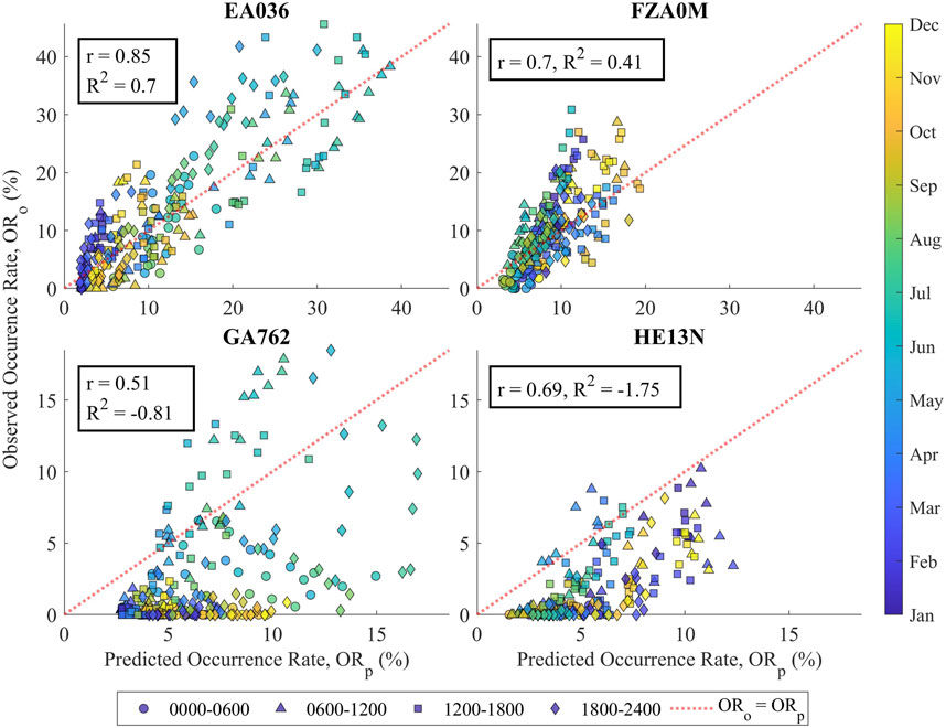
Figure 9. Monthly average of hourly (HHMM) fbEs ORs observed at each site plotted against the monthly average of hourly fbEs ORs predicted for each site. Pearson’s correlation coefficient, $r$, and coefficient of determination, $R^2$, are displayed in each plot. p-values are $<10^{-2}$ for $r$ at each site. The model shows good agreement at El Arenosillo and Fortaleza and consistently overestimates at Gakona and Hermanus but on a small absolute scale.

The typical seasonal trends were observed for El Arenosillo and Hermanus. These mid-latitude locations also appear to have followed the expected semidiurnal trend of morning and afternoon peaks, as indicated by the triangles and squares in Figure 9. For Hermanus and Gakona, the model was overly cautious as it generally predicted higher probabilities of fbEs than actually occurred. The correlation coefficients, $r$, are also shown, and it is interesting to note that while El Arenosillo had observations and predictions over the greatest range (0%–40% OR), it also had the highest $r$ value of 0.85 and the highest coefficient of determination, $R^2$, of 0.70. Gakona had the weakest correlation with $r=0.51$ and $R^2=-0.81$, but as mentioned before, most of the model outputs were within 10% OR of the observed OR. Although not desirable, an $R^2<0$ simply indicates that the model performed worse than a hypothetical model that only predicts the mean value. In other words, a negative $R^2$ indicates a bias in the model. This is evident with the prevalence of observed 0$\%$ ORs, whereas the model generally always outputs a nonzero OR, resulting in a large relative difference between averages of the observed and predicted ORs. While Hermanus and Gakona produced negative $R^2$ values from slight positive biases, model predictions from both sites showed moderate correlations with ionosonde observations, indicating that general data trends are similar. It should be noted that the $R^2$ value reported here corresponds to model predictions compared against a validation dataset where the error is the distance to the one:one line (red dashed line in Figure 9). This $R^2$ is not the same as the coefficient of determination provided for a linear regression between datasets (see Nakagawa and Schielzeth (2013) for a discussion of various $R^2$ interpretations).

Although Figure 9 provides a clear view of the monthly averaged model performance, it does not show the diurnal variations. Figure 10 shows the monthly averaged profiles as a function of local solar time compared to averaged ionosonde observations. Figure 10 also highlights the scales that must be considered when analyzing the accuracy of the model. There is considerably more variance in the fbEs OR for El Arenosillo and Fortaleza, and the model appears to generally match the observed trends. Specifically, for El Arenosillo, the model appears to underestimate peaks and overestimate the valleys but retains the trend and the overall increase that occurs in the summer. For Fortaleza, the model, on average, underestimates the OR, as shown in Figure 9. The consistent overestimation for Gakona and Hermanus was also apparent, but the errors were rarely greater than 10%, which makes them rather small on an absolute scale.

Figure 10

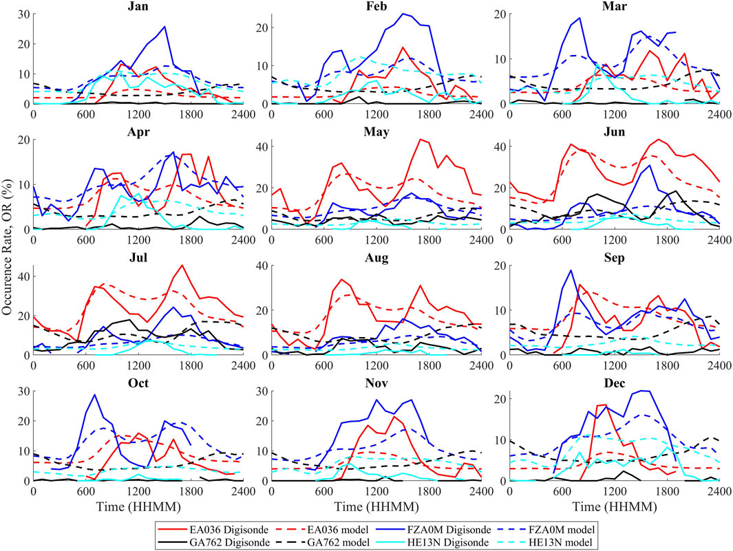
Figure 10. Monthly local solar time occurrence rates at each digisonde site, as observed by the digisonde and predicted by the model. Note the change in scale on the y-axis throughout, and hours that did not satisfy $n_t\ge 4$ are removed from the digisonde plots to illustrate gaps in the observational data. The model generally captures trends but consistently underestimates peak ORs while generally overestimating ORs at non-peak times of the day.

The error was examined in several different ways. First, the mean absolute error (MAE) over different dimensions for each digisonde site was examined (Figure 11). When examining the monthly error, El Arenosillo and Fortaleza clearly show a higher average error, and this was especially true in the summer for El Arenosillo. Fortaleza appears to have a lower average error in the summer than in the winter. Gakona follows a pattern similar to that of El Arenosillo but has much lower average error values. Hermanus has the lowest average error values by month and by hour, with slightly higher errors during the daytime hours. This is shown in Figure 10 and is due to a consistent overestimation of the OR values. Gakona has a higher average error during the late-night hours, while the remaining two stations have a significantly higher error during the daytime hours, particularly in the late afternoon. Fortaleza stands out with the highest average error.

Figure 11

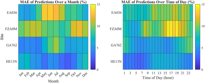
Figure 11. Mean absolute error of model outputs over different dimensions at each digisonde location. Left: MAE for each month. Right: MAE for each hour. Increases in MAE generally correspond to seasonal or daily OR peaks for each location.

The second way in which the error was examined was by comparing error distributions. Figure 12 displays a histogram of the error when comparing the hourly model predictions with the observations for all four sites. Note that only the hours meeting the observation threshold are displayed, and the percentage removed is shown in the legend. This discussion assumes that the unobserved hours follow the same distribution. The standard deviation of the hour-to-hour comparison is 11%. We can see that $\sim 94\%$ of the errors are less than 20% and $\sim 80\%$ are less than 10%. This matches what was visually observed in Figure 9. We can also see that on an hour-to-hour basis, the model is more likely to overestimate, but very large errors tend to be drastic underestimates. Only $\sim$1/20 predictions are drastic underestimates, and they are likely the result of applying the Gaussian filter to the original data.

Figure 12

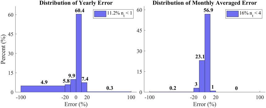
Figure 12. Histograms of the residual error. Left: hour-to-hour error (predicted vs. observed) over the entire year. Right: error when comparing the hourly occurrence rates when each hour is averaged over each month. Errors are generally overestimates, but large errors are large underestimates.

Looking at the errors from monthly averaged comparisons shows that they are much more tightly distributed than would be expected considering how the model was developed. However, this comparison also excludes much more data, as seen by the increase in the percentage of hours in which the observation threshold was not met ($\sim 40\%$ increase). Even if all the unobserved time periods result in an absolute error of 20% or more, nearly 85% of predictions would be within 20% OR and 80% within 10% OR.

Given the initial calculated average uncertainty of 12%, 95% of predictions are expected to have an error of less than 24% $(\sim 2\sigma )$. This approximately matches the error histogram for the hour-to-hour standard deviation of 11%, as well as the initial set standard error of 10%. Considering the agreement between these three determined uncertainty values (12%, 11%, and 10%), it can be safely stated that the model generally has an uncertainty of 12% for specific predictions. In other words, 95% of the outputs will be within 24%. If one is seeking to understand more general or average behavior on a timescale of a month, the model is more accurate.

4 Discussion

The overarching goal of increasing the monthly climatological OR temporal resolution outlined by Hodos et al. (2022) was accomplished through an interpolation of the monthly KLE eigenvalues (Figures 3, 4). This process maintains the OR values for each month while providing estimates between the known periods. Gaussian smoothing of the original datasets helps reduce discontinuities typically found over ionosonde locations where the ionosonde-derived ORs did not match the surrounding GNSS-RO-derived ORs. Finally, the self-consistent combination of temporal and spatial results outlined in Equations 2–5 ensures that the local solar time structures are maintained, while the daily averages match the input spatial maps. In this respect, GEMSOR successfully provides fbEs $\ge$ 3-MHz ORs with hourly time resolution that are consistent with the results obtained by Hodos et al. (2022), thereby extending the dataset for practical use as a model.

A minimum total observation threshold was used to limit the standard error to 10%, as outlined in Hodos et al. (2022), and this appears to have been effective. Propagation of the standard deviation of the individual bins through the combination algorithm and addition of the mean error of the Gaussian filter resulted in an estimated uncertainty of $\sim 9\%$. Comparing the predictions to digisonde observations from a time period not utilized by the model resulted in a monthly averaged standard deviation of 5% and an hourly standard deviation of 11%. All of these values were in relative agreement and indicate that only 1 in 20 predictions should have an error of more than 21%. The monthly averaged standard deviation indicates that if predictions were made for a given hour on every day of the month, the mean of the predictions will be within 10% of the actual mean 95% of the time.

Hermanus and Gakona not only had lower correlation coefficients compared to the other sites when analyzing the monthly averaged data but also a lower MAE when averaging over a month or over an hour. For Hermanus, this is likely due to the rather depressed fbEs in this region due to the proximity of the South Atlantic Anomaly (Arras et al., 2008). The model performed well at the mid-latitude location El Arenosillo, where it generally followed the observed semidiurnal behavior throughout the year. This location also had the highest correlation coefficient but also some of the higher MAEs, particularly in the summer. This error averaged to approximately 15% during its peak in the summer and not much more than 10% when examined hourly. Overall, the model showed strong performance in the mid-latitude region where ${\mathrm{E}}_s$ is known to form more frequently.

In the low-latitude or equatorial region, Fortaleza had the second highest correlation coefficient when averaged over a month. The model generally captured the semidiurnal trends but not as closely as for El Arenosillo. The monthly averaged correlation coefficient was lower, as was the MAE over the entire year. The highest hourly average errors were for Fortaleza, peaking at 15%. It must be noted that while the wind shear mechanism used to describe blanketing ${\mathrm{E}}_s$ formation is maximized with the horizontal magnetic field at the geomagnetic equator (Whitehead, 1989), the magnetized electrons at E-region altitudes (Schunk and Nagy, 2009) are constrained to follow the field lines, which limits blanketing ${\mathrm{E}}_s$ formation in this region. However, equatorial ionosondes frequently measure q-type sporadic-E (Piggott and Rawer, 1972), which is caused by the scattering of HF signals from equatorial electrojet irregularities (Resende et al., 2017; 2018) produced by mechanisms such as the gradient drift instability (Seif and Panda, 2024). While these q-type layers are commonly measured by ionosondes, they do not cause significant impacts to GNSS-RO observations (see Arras et al., 2022b). As the GEMSOR model produced here is tailored to blanketing ${\mathrm{E}}_s$ through a combination of RO and ionosonde observations, comparisons with only ionosonde sporadic-E measurements as the ground truth can be biased in the equatorial region due to these q-type observations, especially with the reliance on automatically scaled ionograms. This may be the cause of the relatively high observed ORs (above the one:one line) for Fortaleza, displayed in the upper-right quadrant of Figure 9. Similarly, there may also be instances where the automatically scaled ionograms from Gakona are falsely attributed to auroral-E as blanketing ${\mathrm{E}}_s$ (Roberts, 2024).

Although the model showed modest success, there are some very important limitations that need to be understood prior to its application. Some locations, particularly geomagnetic latitudes south of 75°S, had an inadequate number of total observations to calculate an OR. The model only predicts 0$\%$ OR at these locations, and the uncertainty will not be reported. Due to the fact that the original calculated ORs are the result of extensive averaging over time and positions, this model will also likely fail to predict short temporal-scale anomalous behavior. Although this anomalous behavior may have existed somewhere in the data, the subsequent averaging probably suppressed its appearance and, as a result, will not be seen in the model. This has already been highlighted by the fact that hour-to-hour comparisons indicated that $\sim 5\%$ of predictions had an error greater than 20$\%$, but monthly average comparisons reduced this to less than $\sim 0.5\%$ of predictions. The model also assumed geomagnetic quiet conditions and defined this as an AE index below 500 nT and a Kp $\le$ 4. ORs during geomagnetic storms are unlikely to be reliably predicted by this model, although the impact of minor geomagnetic activity on sporadic-E appears to be relatively weak at mid-latitudes (Yu et al., 2021). GEMSOR also ignores solar cycle variation, which has been shown to impact ${\mathrm{E}}_s$ formation at high and low latitudes (Whitehead, 1970; Fontes et al., 2024). However, the overall importance of solar and geomagnetic activity on sporadic-E activity is less significant than the location, local time, and day of year [see Figure 3 in the study by Tian et al. (2023)]. While the validation results are encouraging, these four locations hardly cover all possible conditions over the entirety of the globe.

The less number of years in the validation (2019–2022) also limited the number of comparisons that could be made, particularly during local night. Sporadic-E forms primarily during the day with latitude-dependent peaks in either the late morning or early evening (Wu et al., 2005; Chu et al., 2014; Yu et al., 2022). Formation at night, especially during the early-morning hours, is minimal but nonzero with a general increase in mid- and high latitudes during local summer (Luo et al., 2021; Hodos et al., 2022). This behavior is also present in the ionosonde validation dataset displayed in Figure 10. However, many of the nighttime OR calculations for the digisonde sites contained relatively low numbers of observations, which increases the uncertainty in the validation rates at night.

In relation to other empirical ${\mathrm{E}}_s$ models derived from RO observations, GEMSOR shows many similarities while providing a unique output of occurrence rates instead of intensities. For example, Yu et al. (2022) provided an empirical model of ${\mathrm{E}}_s$ intensity based on the maximum ${\mathrm{L}}_1$ amplitude scintillation index, ${\mathrm{S}}_4$-max, which shows the same general spatial, diurnal, and seasonal trends, as predicted by GEMSOR. The inputs to this empirical ${\mathrm{S}}_4$-max model are the same as those input to GEMSOR, with an additional parameter: altitude. While altitude is important to understanding ${\mathrm{E}}_s$ morphology, it is not considered in GEMSOR as the intention is to provide a probabilistic estimate of the impact of ${\mathrm{E}}_s$ on HF operations and not to characterize the intensity or altitude of the layer, as performed by Yu et al. (2022). Similarly, the deep learning Sporadic-E Layer Forecast using Artificial Neural Networks (SELF-ANN) model presented by Tian et al. (2023) provides ${\mathrm{E}}_s$ intensity and altitude predictions with a larger, more sophisticated set of inputs that include neutral wind, tropospheric temperature, and solar and geomagnetic activity. The importance of these additional parameters was not studied by Hodos et al. (2022) and is, therefore, not included in GEMSOR. However, including altitude and other input parameters may help improve model performance in future versions.

For future research, the primary challenge is to improve RO techniques for estimating the existence and strength of sporadic-E layers. Although this is a challenging task due to the integrated nature of the observations, recent studies (Emmons et al., 2023; Ellis et al., 2024) have shown a significant improvement over the baseline techniques compared by Carmona et al. (2022) and applied by Hodos et al. (2022). Implementing these improved RO techniques will improve the OR estimates that form the foundation of the empirical model. Additionally, expanding the validation to more digisonde locations over a greater period will provide further insight into the model’s strengths and weaknesses. Enhancing the spatial resolution would also be beneficial as the current bin size is rather large, especially in the equatorial regions $(\sim 3\times 10^{5}k{m}^2)$. This could be achieved by performing a spatial interpolation on the present model, a spatial interpolation on the data prior to the KLE, or, with more data available, the calculation of fbEs at a higher spatial resolution. The increasing supply of COSMIC II and Spire RO data may soon make the latter option a possibility.

5 Conclusion

This study outlines the development of a GEMSOR through significant enhancements in time resolution from the dataset used by Hodos et al. (2022), which was derived from GNSS-RO and ionosonde observations with an fbEs threshold of 3 MHz. GEMSOR predicts the blanketing sporadic-E OR as a function of geomagnetic latitude, longitude, day of year, and local solar time at a resolution of 5°, 5°, day, and hour, respectively. The results of the model were compared to observations from four digisonde sites, and a general uncertainty of the model was developed. The purpose of this research was to provide a new tool that allows operators of HF equipment to better understand ionospheric conditions for a more effective application of the equipment.

Overall, this study sought to develop an empirical model of global fbEs $\ge$ 3-MHz ORs as a function of position and time, which was achieved at a spatial resolution of 5° geomagnetic latitude $\times$ 5° geographic longitude with an hourly time resolution for each day of year. The uncertainty calculation suggested an average uncertainty of $12\%$, with unique values reported for each output. This was well correlated with the determined average error from validation (11$\%$) and the standard error of 10$\%$ established via the observation threshold. Given the satisfactory performance of this global empirical model of blanketing sporadic-E, we recommend that HF operators utilize this model to inform their operations. Considering the importance of HF applications in communication and surveillance technologies, the development and refinement of such models will continue to be worthwhile for scientific and commercial investment.

Data availability statement

The original contributions presented in the study are included in the article/Supplementary Material; further inquiries can be directed to the corresponding authors.

Author contributions

EP: conceptualization, formal analysis, investigation, writing–original draft, and writing–review and editing. AF: formal analysis, investigation, and writing–original draft. ED: conceptualization, formal analysis, investigation, and writing–original draft. DW: conceptualization, formal analysis, investigation, and writing–original draft. NS: formal analysis, investigation, and writing–original draft. CS: conceptualization, formal analysis, investigation, and writing–original draft. DE: conceptualization, formal analysis, investigation, writing–original draft, and writing–review and editing.

Funding

The author(s) declare that financial support was received for the research, authorship, and/or publication of this article. This research was funded by the Air Force Office of Scientific Research (AFOSR/RTB1), and NASA’s Living With Star and Sun-Climate research funds to the Goddard Space Flight Center (GSFC) under WBS 936723.02.01.12.48.

Acknowledgments

The authors acknowledge the Digital Ionogram Database (https://giro.uml.edu/didbase/) and the COSMIC Data Analysis and Archive Center (https://cdaac-www.cosmic.ucar.edu/) for the use of their data. The views, opinions, and/or findings expressed are those of the authors and should not be interpreted as representing the official views or policies of the Department of Defense or the US Government.

Conflict of interest

The authors declare that the research was conducted in the absence of any commercial or financial relationships that could be construed as a potential conflict of interest.

Publisher’s note

All claims expressed in this article are solely those of the authors and do not necessarily represent those of their affiliated organizations, or those of the publisher, the editors, and the reviewers. Any product that may be evaluated in this article, or claim that may be made by its manufacturer, is not guaranteed or endorsed by the publisher.

Supplementary material

The Supplementary Material for this article can be found online at: https://www.frontiersin.org/articles/10.3389/fspas.2024.1434367/full#supplementary-material

References

Arras, C., Resende, L. C. A., Kepkar, A., Senevirathna, G., and Wickert, J. (2022a). Sporadic E layer characteristics at equatorial latitudes as observed by GNSS radio occultation measurements. Earth, Planets Space 74, 163. doi:10.1186/s40623-022-01718-y

CrossRef Full Text | Google Scholar

Arras, C., Resende, L. C. A., Kepkar, A., Senevirathna, G., and Wickert, J. (2022b). Sporadic e layer characteristics at equatorial latitudes as observed by gnss radio occultation measurements. Earth, Planets Space 74, 163. doi:10.1186/s40623-022-01718-y

CrossRef Full Text | Google Scholar

Arras, C., and Wickert, J. (2018). Estimation of ionospheric sporadic E intensities from GPS radio occultation measurements. J. Atmos. Solar-Terrestrial Phys. 171, 60–63. Vertical Coupling in the Atmosphere-Ionosphere System: Recent Progress. doi:10.1016/j.jastp.2017.08.006

CrossRef Full Text | Google Scholar

Arras, C., Wickert, J., Beyerle, G., Heise, S., Schmidt, T., and Jacobi, C. (2008). A global climatology of ionospheric irregularities derived from gps radio occultation. Geophys. Res. Lett. 35. doi:10.1029/2008GL034158

CrossRef Full Text | Google Scholar

Björnsson, H., and Venegas, S. (1997). A manual for EOF and SVD analyses of climatic data. CCGCR Rep. 97, 112–134.

Google Scholar

Cameron, T., Fiori, R., Themens, D., Warrington, E., Thayaparan, T., and Galeschuk, D. (2022). Evaluation of the effect of sporadic-E on high frequency radio wave propagation in the arctic. J. Atmos. Solar-Terrestrial Phys. 228, 105826. doi:10.1016/j.jastp.2022.105826

CrossRef Full Text | Google Scholar

Carmona, R. A., Nava, O. A., Dao, E. V., and Emmons, D. J. (2022). A comparison of sporadic-E occurrence rates using GPS radio occultation and ionosonde measurements. Remote Sens. 14, 581. doi:10.3390/rs14030581

CrossRef Full Text | Google Scholar

Cathey, E. H. (1969). Some midlatitude sporadic-e results from the explorer 20 satellite. J. Geophys. Res. 74, 2240–2247. doi:10.1029/ja074i009p02240

CrossRef Full Text | Google Scholar

Chartier, A. T., Hanley, T. R., and Emmons, D. J. (2022). Long-distance propagation of 162 mhz shipping information links associated with sporadic e. Atmos. Meas. Tech. 15, 6387–6393. doi:10.5194/amt-15-6387-2022

CrossRef Full Text | Google Scholar

Chu, Y. H., Wang, C. Y., Wu, K. H., Chen, K. T., Tzeng, K. J., Su, C. L., et al. (2014). Morphology of sporadic E layer retrieved from COSMIC GPS radio occultation measurements: wind shear theory examination. J. Geophys. Res. Space Phys. 119, 2117–2136. doi:10.1002/2013JA019437

CrossRef Full Text | Google Scholar

Chulliat, A., Brown, W., Alken, P., Beggan, C., Nair, M., Cox, G., et al. (2020). “The US/UK world magnetic model for 2020-2025: technical report,”. NOAA: National Centers for Environmental Information.

Google Scholar

Ellis, J., Emmons, D., and Cohen, M. (2024). Detection and classification of sporadic e using convolutional neural networks. Space weather. 22, e2023SW003669. doi:10.1029/2023sw003669

CrossRef Full Text | Google Scholar

Emmons, D. J., Wu, D. L., and Swarnalingam, N. (2022). A statistical analysis of sporadic-e characteristics associated with gnss radio occultation phase and amplitude scintillations. Atmosphere 13, 2098. doi:10.3390/atmos13122098

CrossRef Full Text | Google Scholar

Emmons, D. J., Wu, D. L., Swarnalingam, N., Ali, A. F., Ellis, J. A., Fitch, K. E., et al. (2023). Improved models for estimating sporadic-e intensity from gnss radio occultation measurements. Front. Astronomy Space Sci. 10, 1327979. doi:10.3389/fspas.2023.1327979

CrossRef Full Text | Google Scholar

Fontes, P., Muella, M., Resende, L., and Fagundes, P. (2024). Evidence of anti-correlation between sporadic (es) layers occurrence and solar activity observed at low latitudes over the brazilian sector. Adv. Space Res. 73, 3563–3577. doi:10.1016/j.asr.2023.09.040

CrossRef Full Text | Google Scholar

Gooch, J. Y., Colman, J. J., Nava, O. A., and Emmons, D. J. (2020). Global ionosonde and GPS radio occultation sporadic-E intensity and height comparison. J. Atmos. Solar-Terrestrial Phys. 199, 105200. doi:10.1016/j.jastp.2020.105200

CrossRef Full Text | Google Scholar

Haldoupis, C., Pancheva, D., Singer, W., Meek, C., and MacDougall, J. (2007). An explanation for the seasonal dependence of midlatitude sporadic E layers. J. Geophys. Res. Space Phys. 112. doi:10.1029/2007JA012322

CrossRef Full Text | Google Scholar

Headrick, J. M., Anderson, S. J., and Skolnik, M. (2008). HF over-the-horizon radar. Radar Handb. 20.

Google Scholar

Hodos, T. J., Nava, O. A., Dao, E. V., and Emmons, D. J. (2022). Global sporadic-E occurrence rate climatology using GPS radio occultation and ionosonde data. J. Geophys. Res. Space Phys. 127. doi:10.1029/2022ja030795

CrossRef Full Text | Google Scholar

Hysell, D., Nossa, E., Larsen, M., Munro, J., Sulzer, M., and González, S. (2009). Sporadic e layer observations over arecibo using coherent and incoherent scatter radar: Assessing dynamic stability in the lower thermosphere. J. Geophys. Res. Space Phys. 114. doi:10.1029/2009ja014403

CrossRef Full Text | Google Scholar

Kamide, Y., and Akasofu, S. I. (1983). Notes on the auroral electrojet indices. Rev. Geophys. 21, 1647–1656. doi:10.1029/RG021i007p01647

CrossRef Full Text | Google Scholar

Kintner, P. M., Ledvina, B. M., and de Paula, E. R. (2007). GPS and ionospheric scintillations. Space weather. 5. doi:10.1029/2006SW000260

CrossRef Full Text | Google Scholar

Kirby, M. (2000). Geometric data analysis: an empirical approach to dimensionality reduction and the study of patterns. John Wiley and Sons, Inc.

Google Scholar

Ku, H. H., et al. (1966). Notes on the use of propagation of error formulas. J. Res. Natl. Bureau Stand. 70.

CrossRef Full Text | Google Scholar

Kunduri, B. S. R., Erickson, P. J., Baker, J. B., Ruohoniemi, J. M., Galkin, I., and Sterne, K. (2023). Dynamics of mid-latitude sporadic-e and its impact on hf propagation in the north american sector. J. Geophys. Res. Space Phys. 128, e2023JA031455. doi:10.1029/2023ja031455

CrossRef Full Text | Google Scholar

Luo, J., Liu, H., and Xu, X. (2021). Sporadic e morphology based on cosmic radio occultation data and its relationship with wind shear theory. Earth, Planets Space 73, 212–217. doi:10.1186/s40623-021-01550-w

CrossRef Full Text | Google Scholar

MacDougall, J., Jayachandran, P., and Plane, J. (2000). Polar cap sporadic-E: part 1, observations. J. Atmos. Solar-Terrestrial Phys. 62, 1155–1167. doi:10.1016/s1364-6826(00)00093-6

CrossRef Full Text | Google Scholar

Maeda, J., and Heki, K. (2015). Morphology and dynamics of daytime mid-latitude sporadic-e patches revealed by gps total electron content observations in Japan. Earth, Planets Space 67, 89–9. doi:10.1186/s40623-015-0257-4

CrossRef Full Text | Google Scholar

Mathews, J. (1998). Sporadic E: current views and recent progress. J. Atmos. Solar-Terrestrial Phys. 60, 413–435. doi:10.1016/s1364-6826(97)00043-6

CrossRef Full Text | Google Scholar

Maus, S., Macmillan, S., McLean, S., Hamilton, B., Thomson, A., Nair, M., et al. (2010). “The US/UK world magnetic model for 2010-2015,”. Keyworth, Nottinghamshire, England: British Geological Survey.

Google Scholar

McNamara, L. F. (1991). The ionosphere: communications, surveillance, and direction finding. Malabar, Florida: Krieger publishing company.

Google Scholar

Merriman, D. K., Nava, O. A., Dao, E. V., and Emmons, D. J. (2021). Comparison of seasonal foEs and fbEs occurrence rates derived from global Digisonde measurements. Atmosphere 12, 1558. doi:10.3390/atmos12121558

CrossRef Full Text | Google Scholar

Nakagawa, S., and Schielzeth, H. (2013). A general and simple method for obtaining r2 from generalized linear mixed-effects models. Methods Ecol. Evol. 4, 133–142. doi:10.1111/j.2041-210x.2012.00261.x

CrossRef Full Text | Google Scholar

Neubeck, K. (1996). Using the combined resources of amateur radio observations and ionosonde data in the study of temperate zone sporadic-E. J. Atmos. Terr. Phys. 58, 1355–1365. doi:10.1016/0021-9169(95)00170-0

CrossRef Full Text | Google Scholar

Niu, J., Weng, L. B., Meng, X., and Fang, H. X. (2019). Morphology of ionospheric sporadic-E layer intensity based on COSMIC occultation data in the midlatitude and low-latitude regions. J. Geophys. Res. Space Phys. 124, 4796–4808. doi:10.1029/2019JA026828

CrossRef Full Text | Google Scholar

Obenberger, K., Dowell, J., Fallen, C., Holmes, J., Taylor, G., and Varghese, S. (2021). Using broadband radio noise from power-lines to map and track dense E_s structures. Radio Sci. 56, 1–17. doi:10.1029/2020rs007169

CrossRef Full Text | Google Scholar

Piggott, W. R., and Rawer, K. (1972). U.R.S.I. handbook of ionogram interpretation and reduction

Google Scholar

Reddy, C., and Mukunda Rao, M. (1968). On the physical significance of the es parameters fbes, fes, and foes. J. Geophys. Res. 73, 215–224. doi:10.1029/ja073i001p00215

CrossRef Full Text | Google Scholar

Resende, L. C., Arras, C., Batista, I. S., Denardini, C. M., Bertollotto, T. O., and Moro, J. (2018). Study of sporadic e layers based on gps radio occultation measurements and digisonde data over the brazilian region. Ann. Geophys. 36, 587–593. doi:10.5194/angeo-36-587-2018

CrossRef Full Text | Google Scholar

Resende, L. C. A., Batista, I. S., Denardini, C. M., Batista, P. P., Carrasco, A. J., de Fátima Andrioli, V., et al. (2017). Simulations of blanketing sporadic e-layer over the brazilian sector driven by tidal winds. J. Atmos. Solar-Terrestrial Phys. 154, 104–114. doi:10.1016/j.jastp.2016.12.012

CrossRef Full Text | Google Scholar

Roberts, K. D. (2024). Investigation of high-latitude GNSS radio occultation sporadic-E and auroral-E measurements (Air Force Institute of Technology). Wright-Patterson AFB, Dayton OH: Master’s Thesis.

Google Scholar

Schunk, R., and Nagy, A. (2009). Ionospheres: physics, plasma physics, and chemistry. Cambridge University Press.

Google Scholar

Seif, A., and Panda, S. K. (2024). Characterizing global equatorial sporadic-e layers through cosmic gnss radio occultation measurements. Astrophysics Space Sci. 369, 60. doi:10.1007/s10509-024-04326-2

CrossRef Full Text | Google Scholar

Smith, E. K. (1957). Worldwide occurrence of sporadic E, 582. Gaithersburg, Maryland: US Department of Commerce, National Bureau of Standards.

Google Scholar

Stankov, S. M., Verhulst, T. G. W., and Sapundjiev, D. (2023). Automatic ionospheric weather monitoring with DPS-4D ionosonde and ARTIST-5 autoscaler: System performance at a mid-latitude observatory. Radio Sci. 58, 1–20. doi:10.1029/2022RS007628

CrossRef Full Text | Google Scholar

Sun, W., Zhao, X., Hu, L., Yang, S., Xie, H., Chang, S., et al. (2021). Morphological characteristics of thousand-kilometer-scale es structures over China. J. Geophys. Res. Space Phys. 126, e2020JA028712. doi:10.1029/2020ja028712

CrossRef Full Text | Google Scholar

Thayaparan, T., and MacDougall, J. (2005). Evaluation of ionospheric sporadic-E clutter in an arctic environment for the assessment of high-frequency surface-wave radar surveillance. IEEE Trans. geoscience remote Sens. 43, 1180–1188. doi:10.1109/tgrs.2005.844661

CrossRef Full Text | Google Scholar

Tian, P., Yu, B., Ye, H., Xue, X., Wu, J., and Chen, T. (2023). Ionospheric irregularities reconstruction using multi-source data fusion via deep learning. EGUsphere 2023, 1–26. doi:10.5194/egusphere-2023-1304

CrossRef Full Text | Google Scholar

Whitehead, J. (1970). Production and prediction of sporadic e. Rev. Geophys. 8, 65–144. doi:10.1029/rg008i001p00065

CrossRef Full Text | Google Scholar

Whitehead, J. (1989). Recent work on mid-latitude and equatorial sporadic-E. J. Atmos. Terr. Phys. 51, 401–424. doi:10.1016/0021-9169(89)90122-0

CrossRef Full Text | Google Scholar

Wu, D. L., Ao, C. O., Hajj, G. A., de la Torre Juarez, M., and Mannucci, A. J. (2005). sporadic-E morphology from GPS-champ radio occultation. J. Geophys. Res. Space Phys. 110. doi:10.1029/2004JA010701

CrossRef Full Text | Google Scholar

Yu, B., Scott, C. J., Xue, X., Yue, X., Chi, Y., Dou, X., et al. (2021). A signature of 27 day solar rotation in the concentration of metallic ions within the terrestrial ionosphere. Astrophysical J. 916, 106. doi:10.3847/1538-4357/ac0886

CrossRef Full Text | Google Scholar

Yu, B., Scott, C. J., Xue, X., Yue, X., and Dou, X. (2020). Derivation of global ionospheric Sporadic E critical frequency (f o Es) data from the amplitude variations in GPS/GNSS radio occultations. R. Soc. Open Sci. 7, 200320. doi:10.1098/rsos.200320

PubMed Abstract | CrossRef Full Text | Google Scholar

Yu, B., Xue, X., Scott, C. J., Yue, X., and Dou, X. (2022). An empirical model of the ionospheric sporadic E layer based on GNSS radio occultation data. Space weather. 20, e2022SW003113. doi:10.1029/2022sw003113

CrossRef Full Text | Google Scholar

Yue, X., Schreiner, W. S., Pedatella, N. M., and Kuo, Y.-H. (2016). Characterizing GPS radio occultation loss of lock due to ionospheric weather. Space weather. 14, 285–299. doi:10.1002/2015SW001340

CrossRef Full Text | Google Scholar

Zeng, Z., and Sokolovskiy, S. (2010). Effect of sporadic E clouds on GPS radio occultation signals. Geophys. Res. Lett. 37. doi:10.1029/2010GL044561

CrossRef Full Text | Google Scholar