Size Distribution of Emitted Energies in Local Load Sharing Fiber Bundles

We study the local load sharing fiber bundle model and its energy burst statistics. While it is known that the avalanche size distribution of the model is exponential, we numerically show here that the avalanche size (s) and the corresponding average energy burst (〈E〉) in this version of the model have a non-linear relation (〈E〉 ~ s^γ). Numerical results indicate that γ ≈ 2.5 universally for different failure threshold distributions. With this numerical observation, it is then possible to show that the energy burst distribution is a power law, with a universal exponent value of −(γ + 1).

1. Introduction

It is well-known experimentally that quasistatically stressed disordered solids produce intermittent response statistics [1], particularly in terms of acoustic emissions, that show scale-free size distributions. These intriguing dynamics is seen universally across scales from microscopic laboratory samples to the geological scale of earthquakes [2–6]. Empirically, the scale-free size distribution of breaking progression is known in different communities for decades. For example, in geoscience, this is known as the Gutenberg-Richter law, in magnetic domain walls as crackling noise, and so on.

The interests of statistical physicists in this context stems from the universal nature of the dynamics across length and energy scales. The scale-free variations of acoustic emissions, waiting time statistics, etc., are independent of the microscopic details of the underlying systems, which are very different from each other. Such behavior indicates critical dynamics, particularly self-organized critical dynamics for the system, where the universality hypothesis is still applicable, without having to fine-tune a driving parameter [7]. Such a phenomenon is therefore open for analysis with the tools of critical phase transitions, universality and therefore is an important step toward predictability of imminent failure [8–10].

As a consequence of the scale-free dynamics and potential applicability of the universality hypothesis, many generic models were proposed over the years that reproduce such a scale-free behavior. Such models include the fiber bundle model, random spring network, random fuse model, the Burridge-Knopoff model, and so on [5, 11–13]. The common underlying feature of these models is that they are threshold activated, driven, dynamical models. Particularly, for an external driving parameter crossing a pre-assigned threshold value for a single unit of these models, that unit is activated and influences the units in its “neighborhood,” which may in-turn get activated and thereby initiating an “avalanche.” As can be guessed, this type of dynamics is often related to sandpile models of self-organized criticality [14] and indeed such associations extensively explored in the past [15].

The two major parameters that influence the nature of the response in such models are the range of interaction [16] and the strength of the disorder [17, 18]. It was explored, particularly in the fiber bundle model that for a moderate disorder, a scale-free avalanche statistics is only recovered for a “sufficiently” long-range of interaction [16, 19, 20]. In the random fuse model, where the interaction range is not parameters to be tuned, it was shown that the avalanche statistics is not a power-law in the large system size limit [21, 22]. This is in apparent contradiction with the fact that in reality, the interaction range in disordered elastic samples is not infinite i.e., not a mean-field-like interaction. However, experiments routinely reveal scale-free statistics.

One important distinction between the analytical and numerical results of avalanche dynamics and that of the experiments is that in the former it is the number of elements failing in an avalanche that is the measurable quantity, while in the latter it is the energy released in the avalanche. Now, in the mean-field limit of the fiber bundle model, it is straightforward to show that the avalanche size and the energy avalanche size are proportional, hence the two distributions are identical in shape. But this relation is no longer valid for local load sharing variants. In those cases, therefore, it is crucial to explore the size distributions of the energy emissions and compare that with experiments. In this work, we consider the simplest possible variant of the local load sharing fiber bundle model and analyze the energy avalanche statistics of that model. We then compare the results with experiments and also present a plausible argument for its form.

2. Description of Fiber Bundle Model

After being introduced by Pierce [23], the fiber bundle model has been proven to be important yet arguably the simplest model to study failure processes in disordered solids. A conventional fiber bundle model consists of a set of linear elastic fibers or Hookean springs, attached between two parallel plates. The plates are pulled apart by a force F, creating a stress σ = F/L on L fibers. Once the stress crosses the breaking threshold of a particular fiber, chosen from a random distribution, that fiber breaks irreversibly. The stress of broken fibers is then redistributed either globally among all surviving fibers (global load sharing or GLS scheme) or among the surviving nearest neighbors only (local load sharing or LLS scheme). For the GLS scheme [23, 24] no stress concentration occurs anywhere around the failed fibers as the stress of the failed fibers is shared among all surviving fibers. On the other hand, in LLS scheme [25–30], stress concentration is observed near a broken patch (set of neighboring broken fibers) and increases with the size of such patches. After such redistribution, the load per fiber increases initiating failure of more fibers starting an avalanche. At the end of an avalanche, either all fibers are broken (suggesting global failure) or the bundle comes to a stable state with few broken fibers where an increment of external stress is required to make the model evolve further. The last applied stress just before global failure is considered to be the nominal stress or strength σ_c of the bundle. The fraction of fibers that survive at σ_c just before global failure is defined as the critical unbroken fraction of fibers (U_c).

3. Numerical Results

We have studied the fiber bundle model numerically in both mean-field limit and with local load sharing scheme in one dimension, though the major part of the paper will deal with the latter only. Numerical simulations are carried out for system sizes ranging in between 10³ and 10⁷ and are averaged over 10²–10⁴ configurations. Our motive is to understand the dynamics of avalanches and corresponding energy bursts emitted during these avalanches as the model evolves with increasing externally applied stress. Unless otherwise stated, we will use a uniform distribution ranging from 0 to 1 in order to assign threshold values to individual fibers beyond which it breaks.

3.1. Relation Between s and E

Figure 1 shows a comparison between different avalanches and energy emitted during different avalanches for a bundle of size 10⁵. The results are produced for a single configuration. As usual, an avalanche is defined as the number of fibers broken in-between two consecutive stress increments; k is the number of such stress increments in this case. While presenting the energy spectrum and the avalanches we have excluded the final avalanche leading to global failure.

FIGURE 1

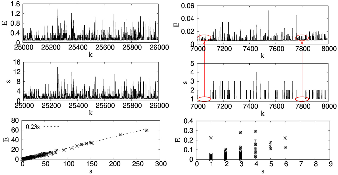
Figure 1. The left panel, from top to bottom, shows the spectrum of energy values (E) with increasing number of avalanches k, avalanche sizes (s) with k and E vs. s for a certain avalanche for a GLS FBM. The right panel does the same but for a LLS FBM. We can see that, in case of a GLS FBM, there is a direct correspondence between the s and E values for a certain k. This means, higher s gives higher E. Since in case of GLS FBM, the fibers break in an increasing order of threshold values, we get, E(k + 1) > E(k) even if s(k + 1) = s(k). We do not see this direct correspondence between the s and E values with local load sharing scheme. For example, the red eclipses show the parts where only 1 fiber breaks at each k value but the corresponding E values show many different values without any particular order as the fibers themselves do not follow any order while breaking. This uncorrelated behavior between s and E.

The left panel of Figure 1 shows the results for the GLS fiber bundle model while on the right panel, we have shown the results with the local load sharing (LLS) scheme. Note that the range of k for the LLS model is much less than the range of k with the GLS scheme. This is understandable since with the LLS scheme, the model is more unstable due to stress concentration and a large number of fibers are broken during the final avalanche. The model evolves with a lesser number of stress increments in this case prior to a global failure where the average size of the avalanches are smaller compared to that in the GLS scheme. Now, for an avalanche of size s, if n fibers with threshold values τ₁, τ₂, τ₃, ⋯ , τ_n break, then the amount of energy emitted during this avalanche will be:

$\begin{array}{ll}E(s)=\frac{1}{2}{\displaystyle \sum _{i=1}^n}{\tau }_i^2.& (1)\end{array}$

This follows from the assumption of linear elastic (stress ∝ strain) behavior of individual fibers up until their individual (brittle) failure points. With above formalism, for each stress increment k, we will obtain an avalanche s(k) and a corresponding energy burst of magnitude E[s(k)].

The energy spectrum follows a particular trend in the case of the GLS scheme. Since with the GLS scheme the fibers break in the increasing order of their threshold values, the energy emitted at k + 1-th load increment will be higher than the energy emitted at k-th increment, even if the avalanche sizes happen to be the same at k and k + 1. Due to this, the variations of s and E with increasing k looks exactly the same, only the values are scaled by a constant when we transfer from s to E. Such correlation between s and E is not present in the case of the LLS fiber bundle model. In the case of the LLS scheme, the fibers break due to the interplay between the local stress profile and the threshold values of the fibers themselves. Due to such dynamics, the fibers do not break in increasing order of their thresholds. Then, there might be scenarios where E(k + 1) < E(k) when s(k + 1) = s(k) or even s(k + 1) > s(k). The red ellipses in the right panel of Figure 1 shows this absence of correlation between s(k) and E[s(k)]. For both ellipses, s = 1 for that period. In spite of that, we see a fluctuation in energy values without a particular trend. This can be clearly understood from the lower row of Figure 1 where E is expressed as a function s. Clearly, in case of GLS FBM, E increases in a linear manner with s while for LLS, the values of E and s are completely uncorrelated. In the following, we will discuss this relation between s and E in detail.

Figure 2 highlights how average of emitted energy 〈E〉 behaves as a function of avalanche size s for a bundle of size 10⁵ and configuration 10⁴. Results for both GLS and LLS schemes are shown in the figure. We observe the following behavior:

$\begin{array}{ll}\langle E\rangle \sim \{\begin{array}{ll}s\hfill & ,\text{for GLS},\hfill \\ s^{\gamma }\hfill & ,\text{with }\gamma =2.5\text{ for LLS}.\hfill \end{array}& (2)\end{array}$

FIGURE 2

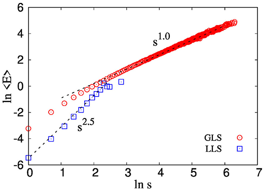
Figure 2. The figure shows the variation of average energy 〈E〉 with avalanche size s for both GLS and LLS fiber bundle model. We observe 〈E〉 ~ s, for GLS FBM. On the other hand, for LLS scheme, 〈E〉 ~ s^γ, with γ ≈ 2.5.

This behavior can be used to understand the relation between distributions P(s) of avalanche size s and Q(〈E〉) of average emitted energies 〈E〉. For this we simply need to implement a change in variable¹ scheme as follows:

$\begin{array}{ll}Q(\langle E\rangle )\sim P\left[s(\langle E\rangle )\right].|s^{\prime }(\langle E\rangle )|=P\left[s(\langle E\rangle )\right].|\frac{ds(\langle E\rangle )}{d\langle E\rangle }|& (3)\end{array}$

Change in variable: GLS scheme

In case of GLS scheme, we observe

$\begin{array}{l}\langle E\rangle (s)\sim s\\ s(\langle E\rangle )\sim \langle E\rangle & (4)\end{array}$

This makes

$\begin{array}{ll}{s}^{\prime }(\langle E\rangle )=\frac{ds(\langle E\rangle )}{d\langle E\rangle }\sim 1& (5)\end{array}$

We also know that the avalanche size distribution in case of GLS scheme is a scale free distribution with an exponent 2.5 [31].

$\begin{array}{ll}P(s)\sim s^{-\beta },\text{with}\beta =2.5& (6)\end{array}$

Then, combining Equations (3), (4), (5), and (6), we get,

$\begin{array}{ll}Q(\langle E\rangle )\sim P(\langle E\rangle ).1\sim {\langle E\rangle }^{-\beta },\text{with}\beta =2.5& (7)\end{array}$

Change in variable: LLS scheme

In case of LLS scheme, we observe

$\begin{array}{l}\langle E\rangle (s)\sim s^{\gamma }\\ s(\langle E\rangle )\sim {\langle E\rangle }^{-\gamma }& (8)\end{array}$

This makes

$\begin{array}{ll}{s}^{\prime }(\langle E\rangle )=\frac{ds(\langle E\rangle )}{d\langle E\rangle }\sim (-\gamma ){\langle E\rangle }^{-(\gamma +1)}& (9)\end{array}$

where γ = 2.5. We also know that the avalanche size distribution in case of LLS scheme is an exponential distribution [32].

$\begin{array}{ll}P(s)\sim e^{-s/s_0}& (10)\end{array}$

Then, combining Equations (3), (8), (9), and (10), we get,

$\begin{array}{ll}Q(\langle E\rangle )\sim P(\langle E\rangle ).\gamma {\langle E\rangle }^{-(\gamma +1)}\sim \gamma e^{-\frac{{\langle E\rangle }^{-\gamma }}{s_0}}{E}^{-(\gamma +1)}& (11)\end{array}$

In the limit of high E value, Equation (11) can be simplified as follows

$\begin{array}{ll}Q(\langle E\rangle )\sim {\langle E\rangle }^{-\alpha }\text{where}\alpha =\gamma +1=3.5& (12)\end{array}$

Above treatment shows that, in case of LLS scheme, in spite of an exponential distribution for avalanche sizes, the distribution of average emitted energy is still observed to be scale-free. Numerically we have found that this scale free behavior holds good for instantaneous values of E as well.

3.2. Distribution of s and E: Uniform Distribution

Figure 3a shows the avalanche size distribution P(s) for a GLS fiber bundle model with system size ranging from 10³ to 10⁵. This scale-free decrease of P(s) with s is already known in the literature. We also observe the same universal exponent 2.5 [31]. Figure 3b shows the corresponding distribution for the energy emitted. We observe the same scale-free distribution for the energy as well, with the same exponent 2.5. This behavior is consistent with Equations (6) and (7), respectively.

FIGURE 3

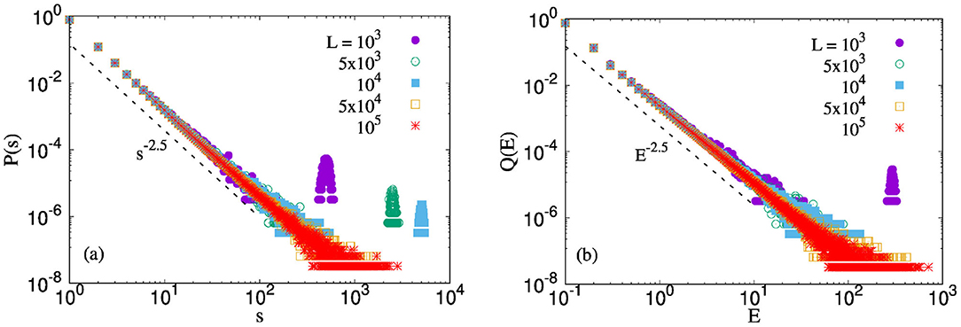
Figure 3. Distribution of energies for an uniform distribution (0,1) and system sizes ranging in between 10³ and 10⁵. The results are shown for GLS FBM. (a) We already know that in the mean-field limit P(s) ∼ s^−β, with β ≈ 2.5. (b) We observe Q(E) ~ E^−α where α ≈ 2.5 as well independent of the system size.

Figure 4a, on the other hand, shows the avalanche size distribution with the LLS scheme. The distribution is exponential as derived analytically by Kloster et al. [32]. The inset of the same results in log scale in order to compare them with the previous claim by Zhang and Ding [33], that P(s) shows a scale-free behavior with a very high exponent closer to −4.8. This claim of scale-free nature is not substantiated and the exponential form for P(s) is accepted in the literature.

FIGURE 4

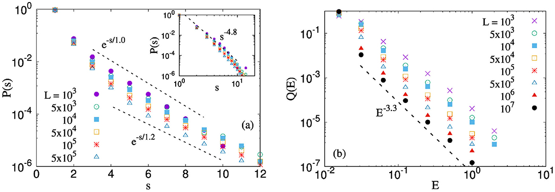
Figure 4. Distribution of energies for an uniform distribution [0:1] and system sizes ranging in between 10³ and 10⁷. The results are shown for LLS FBM. (a) Avalanche size distribution for LLS FBM is an exponential function: $P(s)\sim e^{-s/s_0}$, where s₀ depends weakly on the system size. (b) Scale free distribution for energy emitted: Q(E) ~ E^−α, where α is observed to increase slightly with system size.

The distribution of energy in Figure 4b shows a scale-free distribution, in spite of the fact that the avalanche size distribution is an exponential distribution. The exponent of the scale-free distribution is observed to an increasing function of the size of the bundle

$\begin{array}{ll}Q(E)\sim E^{-\alpha (L)}& (13)\end{array}$

The above behavior is similar to Equation (12), but with a L dependent exponent instead of a constant value. To compare this L dependent exponent with the value in Equation (12), we have to study the variation of α in Equation (13) in details as the size of the bundle is increased. We have discussed this next.

Figure 5 shows the system size scaling of the behavior in Equation (13) as the size of the bundle is increased from 10³ to 10⁷. The behavior of Q(E) in Figure 4b tells us that the slope of the distribution increases and Q(E) itself decreases as we increase the size of the system. We assume this decrease in Q(E) with L to be scale-free in nature and observed a nice collapse for all system sizes. The scaling we adopted is as follows:

$\begin{array}{ll}Q(E)=L^{-\xi }{E}^{-\alpha (L)}& (14)\end{array}$

where α(L) scales to its value in the thermodynamic limit is a scale free behavior: α(L) = α(∞)−L^−η. We will show this scaling explicitly later in this article. Taking logarithmic on both sides of Equation (14) we get,

$\begin{array}{ll}lnQ(E)=-\xi lnL-\left[\alpha (\infty )-L^{-\eta }\right]lnE& (15)\end{array}$

FIGURE 5

Figure 5. (a) The finite size effect of Q(E) is shown for uniform threshold distribution, which follows a scaling: ln Q(E) = −ξ ln L − [α(∞) − L^−η]ln E with η = 0.15, ξ = 0.55, and α(∞) = 3.47. (b) System size scaling of the exponent α as we approach the thermodynamic limit: α(∞) − α(L) ~ L^−η, with η = 0.15 and α(∞) = 3.47. (c,d) The least square fit error as a function of exponent η and α(∞), both with a minimum at a certain value. We consider the value of α(∞) and η which produces the minimum error. This same procedure has been followed next while exploring the same thing for different threshold distributions.

Figure 5a shows a good collapse with the results of Figure 4b using the following values of the fitting parameters: α(∞) = 3.47, η = 0.14, and ξ = 0.55. In addition, Figure 5b also shows the scaling of the exponent α explicitly as the model starts approaching the thermodynamic limit. We observe the following scaling,

$\begin{array}{ll}\alpha (\infty )-\alpha (L)\sim L^{-\eta }& (16)\end{array}$

where η = −0.15 and α(∞) (= 3.47) has a value close to γ + 1 (see Equation 12). The fitting and the exponent η is calculated from the minimization of least square fit error. This is shown in Figures 5c,d. We choose a certain value of η and fit our numerical results. This in turn will produce a value of α(∞) and corresponding least square fit error. The opposite can also be done where we can fix a certain α(∞) value and the least square fit gives us the value of η and error associated with it. If we repeat this for a number of α(∞) or η values, then we can express the error as a function of either of this parameters η (see Figure 5c) or α(∞) (see Figure 5d). The dotted line in Figure 5a corresponds to the value of α(∞) (= 3.47) and η (= 0.15) for which the least square fit error is minimum independent of whether the error is calculated with a constant α(∞) or η.

3.3. Universality

So far, we have generated the numerical results where a uniform distribution from 0 to 1 is used to assign random thresholds to individual fibers. In this section, we will verify the universality of our results. For this purpose, we will mainly explore 4 other distributions: (i) linearly increasing from 0 to 1, (ii) linearly decreasing from 0 to 1, (ii) a Weibull distribution with scale parameter 1 and Weibull modulus 1, and (iii) A power law distribution from 0 to 1 with exponent 2.0.

In all these cases, the energy burst size distributions were found to be scale-free with an exponent value close to −3.5 (see Figures 6a–d), as is predicted from Equation (12). The variation with system size also universal across these different threshold distributions. The insets of Figures 6a–d shows the same scaling given by Equation (15) and observed in Figure 5a. These results suggest that the scale-free nature of the energy burst size distribution in the local load sharing fiber bundle model is a universal feature.

FIGURE 6

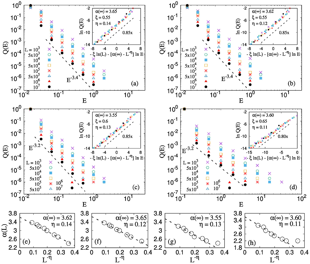
Figure 6. (a) Distribution of energies for four different threshold distributions: (a) Linearly increasing [0:1], (b) Linearly decreasing [0:1], (c) Scale free distribution of exponent 2 between 0 and 1, (d) Weibull distribution with scale factor 1.0 and Weibull modulus 1.0. The system sizes varies in between 10³ and 10⁷. The results are shown for LLS FBM. We observe a scale free distribution for E: Q(E) ~ E^−α for all thresholds. The insets of figures (a–d) shows the system size collapse given by Equation (15). (e–h) Shows the exponent α(L) to obey the scaling showed in Equation 16. The value of η for above mentioned distributions are 0.14, 0.12, 0.13, and 0.11 respectively, similar to what is observed in the system size collapse.

Moreover, Figures 6e–h shows the system size scaling of the exponent α(L) (see Equation 16) for all four threshold distributions: linearly increasing, linearly decreasing, power law and Weibull, respectively.

We have further checked that the relation between an avalanche size and average energy burst size i.e., 〈E〉 ~ s^2.5 is valid for all these threshold distributions, as can be seen from Figure 7. This holds good with the scale-free nature of energy burst distribution that we observed in Equations 6(a)–(d) for all four threshold distributions.

FIGURE 7

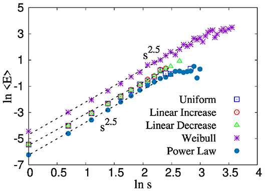
Figure 7. The figure shows the variation of average energy 〈E〉 with avalanche size s for LLS fiber bundle model. We have produced the study for five different threshold distributions. We observe for all distributions, 〈E〉 ~ s^γ, where γ has a value 2.5 independent of the nature of the distribution.

Finally, we have discussed in Table 1, all exponents that we observed in relation to burst size distribution for all five threshold distributions.

TABLE 1

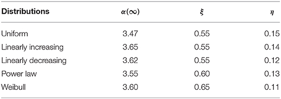
Table 1. The table shows the exponents α(∞) (Equation 16), η (Equation 15), and ξ (Equations 14, 15) related to the system size scaling of the energy size distribution.

4. Discussions and Conclusions

The local load sharing fiber bundle model is known to be lacking in reproducing the scale-free avalanche statistics often seen in the experimental setup of fracturing brittle solids. In all the interpolation schemes between global (equal) and local load sharing versions of fiber bundles, the avalanche size distribution P(s) only show a cross-over between the mean-field (P(s) ∼ s^−β) and local load sharing ($P(s)\sim e^{-s/s_0}$) limits. The mean-field limit, however, is a rather idealized condition for modeling real samples.

However, one important distinction between avalanche sizes (s) of the fiber bundle model and what is usually measured in the experiments is that in the latter case it is the energy burst (E) emitted in an avalanche that is measured. However, that distinction is not at all significant in the mean-field i.e., the global load-sharing limit of the model, because in that limit 〈E〉 ~ s. However, in the local load sharing version, we numerically find 〈E〉 ~ s^γ. Given an exponential nature for the avalanche size distribution in the local load sharing limit and this numerical observation, it is possible to show that the size distribution of the energy bursts is scale-free [Q(〈E〉) ~ 〈E〉^−α] with α = γ + 1 (see Equation 12). Moreover, we have numerically established that this same scale free distribution exists for instantaneous values of the energy emitted and not only for the average emitted energy. We have then numerically checked that γ ≈ 2.5 for various different threshold distributions (see Figure 6) and independently checked that the size distribution exponent for the energy bursts are close to −3.5 (see Figures 4, 7). Indeed, there are indications in experiments with sandstones that the avalanche amplitude distribution was exponential while the energy burst distribution was found to be a power law (see e.g., [34, 35]). Our results reproduce the same for the local load sharing fiber bundle model.

In conclusion, the local load sharing fiber bundle model is shown to have a non-trivial relation between the avalanche size (number of fibers broken) and the energy burst size (elastic energy released from the broken fibers). Consequently, the energy burst size distribution is shown to have scale-free nature, with an exponent value independent of the threshold distributions of the fibers. Given that experimentally one measures the energy released, these results indicate that local load sharing fiber bundles can have a significant role in modeling fracture of brittle solids without having to resort to the equal load sharing mean-field limit.

Data Availability Statement

The raw data supporting the conclusions of this article will be made available by the authors, without undue reservation.

Author Contributions

SR did the numerical simulations. SB has written the first draft of the paper. All authors have edited the manuscript afterwards up to the final version.

Funding

This work was partly supported by the Research Council of Norway through its Centres of Excellence funding scheme, project number 262644.

Conflict of Interest

The authors declare that the research was conducted in the absence of any commercial or financial relationships that could be construed as a potential conflict of interest.

Acknowledgments

The authors thank Prof. Bikas K Chakrabarti and Prof. Purusattam Ray for his valuable comments.

Footnotes

1. ^Let's assume x and y are a continuous functions with p.d.f f(x) and g(y). Also, y = u(x) is a function with inverse, which means it is possible to find x = v(y). In this circumstances, g(y) and f(x) can be expressed as: g(y) = f[v(y)].|v′(y)|, where |v′(y)| = |dv(y)/dy|.

References

1. Bonamy D, Bouchaud E. Failure of heterogeneous materials: a dynamic phase transition? Phys Rep. (2011) 498:1. doi: 10.1016/j.physrep.2010.07.006

CrossRef Full Text | Google Scholar

2. Herrmann H, Roux S, (editors). Statistical Models for the Fracture of Disordered Media. Amsterdam: Elsevier (1990).

Google Scholar

3. Chakrabarti BK, Benguigui L. Statistical Physics of Fracture and Breakdown in Disordered Systems. Oxford: Oxford University Press (1997).

Google Scholar

4. Kawamura H, Hatano T, Kato N, Biswas S, Chakrabarti BK. Statistical physics of fracture, friction, and earthquakes. Rev Mod Phys. (2012) 84:839. doi: 10.1103/RevModPhys.84.839

CrossRef Full Text | Google Scholar

5. Biswas S, Ray P, Chakrabarti BK. Statistical Physics of Fracture, Breakdown, and Earthqauke: Effect of Disorder and Heterogeneity. Singapore: Wiley-VCH (2015).

Google Scholar

6. de Arcangelis L, Godano C, Grasso JR, Lippiello E. Statistical physics approach to earthquake occurrence and forecasting. Phys Rep. (2016) 628:1. doi: 10.1016/j.physrep.2016.03.002

CrossRef Full Text | Google Scholar

7. Bonamy D, Santucci S, Ponson L. Crackling dynamics in material failure as the signature of a self-organized dynamic phase transition. Phys Rev Lett. (2008) 101:045501. doi: 10.1103/PhysRevLett.101.045501

PubMed Abstract | CrossRef Full Text | Google Scholar

8. Koivisto J, Ovaska M, Miksic A, Laurson L, Alava MJ. Predicting sample lifetimes in creep fracture of heterogeneous materials. Phys Rev E. (2016) 94:023002. doi: 10.1103/PhysRevE.94.023002

PubMed Abstract | CrossRef Full Text | Google Scholar

9. Kádár V, Pál G, Kun F. Record statistics of bursts signals the onset of acceleration towards failure. Sci Rep. (2020) 10:2508. doi: 10.1038/s41598-020-59333-4

PubMed Abstract | CrossRef Full Text | Google Scholar

10. Biswas S, Castellanos DF, Zaiser M. Prediction of creep failure time using machine learning. Sci Rep. (2020) 10:16910. doi: 10.1038/s41598-020-72969-6

PubMed Abstract | CrossRef Full Text | Google Scholar

11. Pradhan S, Hansen A, Chakrabarti BK. Failure processes in elastic fiber bundles. Rev Mod Phys. (2010) 82:499. doi: 10.1103/RevModPhys.82.499

CrossRef Full Text | Google Scholar

12. Hansen A, Hemmer PC, Pradhan S. The Fiber Bundle Model: Modeling Failure in Materials. Singapore: Wiley-VCH (2015).

Google Scholar

13. Ray P, Date G. Spatial scaling in fracture propagation in dilute systems. Physica A. (1996) 229:26. doi: 10.1016/0378-4371(95)00431-9

CrossRef Full Text | Google Scholar

14. Bak P, Tang C, Wiesenfeld K. Self-organized criticality: an explanation of 1/f noise. Phys Rev Lett. (1987) 59:381. doi: 10.1103/PhysRevLett.59.381

PubMed Abstract | CrossRef Full Text | Google Scholar

15. Pradhan S, Chakrabarti BK. Precursors of catastrophe in the Bak-Tang-Wiesenfeld, Manna, and random-fiber-bundle models of failure. Phys Rev E. (2001) 65:016113. doi: 10.1103/PhysRevE.65.016113

PubMed Abstract | CrossRef Full Text | Google Scholar

16. Biswas S, Roy S, Ray P. Nucleation versus percolation: Scaling criterion for failure in disordered solids. Phys Rev E. (2015) 91:050105. doi: 10.1103/PhysRevE.91.050105

PubMed Abstract | CrossRef Full Text | Google Scholar

17. Roy S, Ray P. Critical behavior in fiber bundle model: A study on brittle to quasi-brittle transition. Europhys. Lett. (2015) 112:26004. doi: 10.1209/0295-5075/112/26004

CrossRef Full Text | Google Scholar

18. Sinha S, Roy S, Hansen A. Phase transitions and correlations in fracture process where disorder and stress compete. Phys. Rev. Research, (2020) 2:043108. doi: 10.1103/PhysRevResearch.2.043108

CrossRef Full Text | Google Scholar

19. Roy S, Biswas S, Ray P. Modes of failure in disordered solids. Phys Rev E. (2017) 96:063003. doi: 10.1103/PhysRevE.96.063003

CrossRef Full Text | Google Scholar

20. Kun F, Pál G, Varga I, Main IG. Effect of disorder on the spatial structure of damage in slowly compressed porous rocks. Philos Trans R Soc A. (2019) 377:20170393. doi: 10.1098/rsta.2017.0393

PubMed Abstract | CrossRef Full Text | Google Scholar

21. Shekhawat A, Zapperi S, Sethna JP. From damage percolation to crack nucleation through finite size criticality. Phys Rev Lett. (2013) 110:185505. doi: 10.1103/PhysRevLett.110.185505

PubMed Abstract | CrossRef Full Text | Google Scholar

22. Moreira AA, Oliveira CLN, Araujo NAM, Herrmann HJ, Andrade JS. Fracturing highly disordered Materials. Phys. Rev. Lett, (2012) 109:255701. doi: 10.1103/PhysResLett.109.255701

CrossRef Full Text | Google Scholar

23. Pierce FT. Tensile tests for cotton yarns, “The weakest link" theorems on the strength of long and composite specimens. J Text Inst. (1926) 17:355. doi: 10.1080/19447027.1926.10599953

CrossRef Full Text

24. Daniels HE. The statistical theory of strength of bundles of threads. Proc R Soc Lond Ser A. (1945) 183:405. doi: 10.1098/rspa.1945.0011

CrossRef Full Text | Google Scholar

25. Phoenix SL. The asymptotic distribution for the time to failure of a fiber bundle. Adv Appl Probab. (1979) 11:153. doi: 10.1017/S0001867800031748

CrossRef Full Text | Google Scholar

26. Smith RL, Phoenix SL. Asymptotic distributions for the failure of fibrous materials under series-parallel structure and equal load-sharing. J Appl Mech. (1981) 48:75. doi: 10.1115/1.3157595

CrossRef Full Text | Google Scholar

27. Newman WI, Phoenix SL. Time-dependent fiber bundles with local load sharing. Phys Rev E. (2001) 63:021507. doi: 10.1103/PhysRevE.63.021507

PubMed Abstract | CrossRef Full Text | Google Scholar

28. Harlow DG, Phoenix SL. The chain-of-bundles probability model for the strength of fibrous materials I: analysis and conjectures. J Compos Mater. (1978) 12:314. doi: 10.1177/002199837801200308

CrossRef Full Text | Google Scholar

29. Harlow DG, Phoenix SL. Probability distributions for the strength of fibrous materials under local load sharing I: two-level failure and edge effects. Adv Appl Probab. (1982) 14:68. doi: 10.1017/S0001867800036715

CrossRef Full Text | Google Scholar

30. Smith RL. Proc R Soc Lond Ser A. (1982) 382:179. doi: 10.1098/rspa.1982.0095

CrossRef Full Text

31. Kloster M, Hansen A, Hemmer PC. Burst avalanches in solvable models of fibrous materials. Phys Rev E. (1997) 56:2615. doi: 10.1103/PhysRevE.56.2615

CrossRef Full Text | Google Scholar

32. Hammer PC, Hansen A. The distribution of simultaneous fiber failures in fiber bundles. ASME J Appl Mech. (1992) 59:909. doi: 10.1115/1.2894060

CrossRef Full Text | Google Scholar

33. Zhang SD, Ding EJ. Burst-size distribution in fiber-bundles with local load-sharing. Phys Lett A. (1994) 193:425. doi: 10.1016/0375-9601(94)90534-7

CrossRef Full Text | Google Scholar

34. Pradhan S, Stroisz AM, Fjær E, Lund HK, Sønstebø EF, Roy S. Fracturing tests on reservoir rocks: analysis of AE events and radial strain evolution. 48th US Rock Mechanics/Geomechanics Symposium Proceedings, American Rock Mechanics Association (ARMA). (2014) 14:7442.

Google Scholar

35. Pradhan S, Stroisz AM, Fjær E, Stenebråten JF, Lund HK, Sønstebø EV. Stress-induced fracturing of reservoir rocks: Acoustic monitoring and μCT image analysis. Rock Mech Rock Eng. (2015) 48:2529. doi: 10.1007/s00603-015-0853-4

CrossRef Full Text | Google Scholar