
95% of researchers rate our articles as excellent or good
Learn more about the work of our research integrity team to safeguard the quality of each article we publish.
Find out more
REVIEW article
Front. Phys. , 15 February 2021
Sec. Interdisciplinary Physics
Volume 8 - 2020 | https://doi.org/10.3389/fphy.2020.613392
This article is part of the Research Topic The Fiber Bundle View all 12 articles
We discuss the cooperative failure dynamics in the fiber bundle model where the individual elements or fibers are Hookean springs that have identical spring constants but different breaking strengths. When the bundle is stressed or strained, especially in the equal-load-sharing scheme, the load supported by the failed fiber gets shared equally by the rest of the surviving fibers. This mean-field-type statistical feature (absence of fluctuations) in the load-sharing mechanism helped major analytical developments in the study of breaking dynamics in the model and precise comparisons with simulation results. We intend to present a brief review on these developments.
Fiber bundle model (FBM) has been used widely for studying the fracture and failure [1] of composite materials under external loading. The simplicity of the model allows us to achieve analytic solutions [2–4] to an extent that is not possible in any other fracture models. For these very reasons, FBM is widely used as a model of breakdown that extends beyond disordered solids. In fact, FBM was first introduced in connection with textile engineering [5]. Physicists took interest in it recently to explore the critical failure dynamics and avalanche phenomena during such stress-induced failures [6–9]. Apart from the classical fracture–failure in composites, FBM has been used successfully for studying noise-induced (creep/fatigue) failure [10–14] where a fixed load is applied on the system and external noise triggers the failure of elements. Furthermore, it was used as a model for other geophysical phenomena, such as snow avalanche [15], land slides [16, 17], biological materials [18], or even earthquakes [19]. In this review article, we concentrate only on the cooperative dynamical aspects in FBM.
F. T. Peirce, a textile engineer, introduced the fiber bundle model [5] in 1926 to study the strength of cotton yarn. Later, in 1945, Daniels discussed some static behavior of such a bundle [20] and the model was brought to the attention of physicists in 1989 by Sornette [21] who started analyzing the failure process. Even though FBM was designed initially as a model for the fracture or failure of a set of parallel elements (fibers), having different breaking thresholds, with a collective load-sharing scheme, the failure dynamics in the model shows all the attributes of the critical phenomena and the associated phase transition. It seems, due to the usefulness and richness, FBM plays the same role (in the field of fracture) as the Ising model in magnetism [22].
In FBM, a number of parallel Hookean springs or fibers are clamped between two horizontal platforms (Figure 1). The breaking strengths of the springs or fibers are different. When the load per fiber (stress) exceeds a fiber’s own threshold, it fails. The load it carries has to be shared by the surviving fibers. If the lower platform deforms under loading while the upper platform remains rigid, fibers in the neighborhood of the just-failed fiber will absorb more of the load compared to fibers sitting further away, and this arrangement is called the local-load-sharing (LLS) scheme [23, 24]. If both the platforms are rigid, the load has to be equally distributed among all the surviving fibers, which is called the equal-load-sharing (ELS) scheme. Intermediate load redistribution schemes are also studied (see, e.g., [25]), where a part of the load is shared locally within a few fibers and the rest is shared globally among all the fibers.
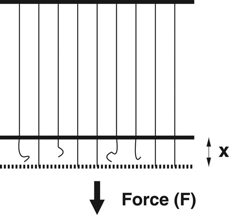
FIGURE 1. A cartoon of the fiber bundle model where a macroscopically large number (N) of Hookean springs, with identical spring constants but different breaking thresholds, hang parallelly from an upper rigid bar and a load/force F is applied at the lower horizontal rigid bar (not allowing any local deformation of the bar and consequent local stress concentration). If any spring fails at any time, the (extra) load is shared by the surviving fibers at that time. In the equal-load-sharing scheme, considered here, this extra load is shared equally by all the surviving fibers (x denoting the strain of the surviving fibers).
How does cooperative dynamics set in? In the case of ELS, all the intact fibers carry the load equally. When a fiber fails, the stress level increases on the remaining fibers and that can trigger more fiber failures (successive failure). As long as the initial load is low, the successive failures of the fibers remain small, and though the strain (stretch) of the bundle grows with increasing stress (load), the bundle as a whole does not fail. Once the initial load reaches a “critical” value, determined by the fiber strength distribution, the successive failures become global (catastrophic) and the bundle collapses.
We arrange this review article as follows: In the short introduction (Section 1), we elaborate the concept of the fiber bundle model and its evolution as a fracture model. Section 2 deals with the equal-load-sharing FBM where we demonstrate the dynamic behavior of FBM with evolution dynamics and their solutions. Analytic results are compared with numerical simulations in this section. In Section 3, we discuss noise-induced failure dynamics in FBM through theory, simulation, and real data analysis. The self-organizing mechanism in FBM is discussed in Section 4. We reserve Section 5 for discussions on some works that would help to understand the cooperative dynamics in FBM. Finally, we have a short Summary and Conclusion section (Section 6) at the end.
We consider an FBM having N parallel fibers placed between two rigid bars. Each fiber follows Hook’s law with a force f to the stretch value x as
Other than the analytical treatment of the model, several aspects of the model are also explored numerically. The implementation of the model, particularly in the equal load sharing version we discuss here, is straightforward. The load is initially applied to each fiber equally. The fibers having failure thresholds less than the applied load are irreversibly broken. The load carried by those fibers is redistributed equally among the remaining fibers, which can cause further breaking. The redistribution continues until no new fibers are breaking. The external load is held constant during the whole redistribution process. This is due to the separation of time scales of externally applied loading rate and the internal (elastic) relaxation processes within materials. After the end of each redistribution cycle, the external load is further increased to continue the dynamics. This process continues until the entire system is broken. The critical strength, avalanche statistics, and other critical exponents are calculated from this dynamics, which, as we will see, match well with the analytical results.
The fiber strength thresholds are drawn from a probability density of
The most used threshold distributions are uniform and Weibull distributions (see Figure 2) in the FBM literature.
For a uniform distribution, we can write
where, the range of function is between 0 and 1. The cumulative Weibull distribution has the form:
where, k is the shape parameter or the Weibull index. The corresponding probability distribution takes the form:
The shapes of the uniform and Weibull distributions are shown in Figure 2. The range of definition is between 0 and
When we stretch the bundle by applying a force, the fibers fail according to their thresholds, the weakest first, then the next weakest, and so on. If
as
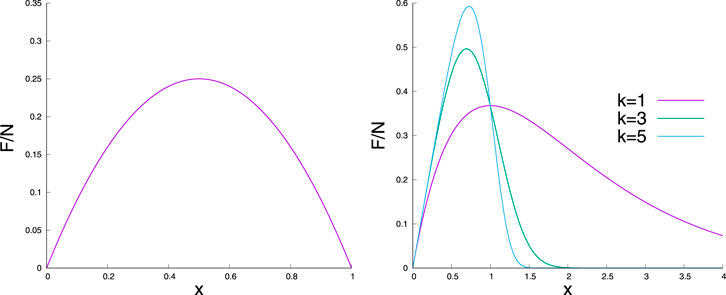
FIGURE 3. Normalized force
It is obvious that the maximum of the force value is the strength of the bundle, and the corresponding stretch value
The critical stretch value can be obtained easily by setting
1. Uniform threshold distribution
Substituting the
Now inserting the
which is the critical strength of the bundle (Figure 3).
2. Weibull threshold distribution
In the case of Weibull distribution, at the force-maximum, by inserting the
One can get the critical stretch value
and the corresponding critical force value
For
Now, we will discuss how the load or stress can be applied on the bundle. In the FBM literature, the most common loading mechanism discussed [26, 27] is the -weakest-link-failure mechanism of loading. This loading process ensures a separation in time scales between external loading and internal stress redistribution. This is equivalent to a quasi-static approach, and noise/fluctuation in the threshold distribution influences the breaking dynamics as well as the avalanche statistics.
A fiber bundle can also be loaded in a different way by applying a fixed amount of load at a time. In that case, all fibers having a failure threshold below the applied load, fail. The stress on the surviving fibers then increases due to load redistribution. The increased stress may drive further failures, and so on. This iterative breaking process continues until an equilibrium is reached where the intact fibers (those who can support the load) is reached. One can also study the failure dynamics of the bundle when the external load on the bundle is then increased infinitesimally, but by a fixed amount (irrespective of the fluctuations in the fiber strength distribution as discussed above). Indeed, as shown recently in Biswas and Chakrabarti [28], the universality class of the dynamics of such fixed loading (even for the same ELS mode of load redistribution after individual fiber failure) will be different from that for the quasi-static (or weakest link failure type) loading discussed above and is given by the Flory statistics [29] for linear polymers, accommodating the Kolmogorov-type dispersion in turbulence [30].
We are going to discuss the cooperative dynamical behavior of the breaking processes for the bundle loaded by fixed amount per step (following the formulations in the References [1, 2, 4, 8, 26, 27, 31]).
Let us assume that an external force F is applied to the fiber bundle. The stress on the bundle (the external load per fiber) is
Let us call
Now, the effective stress becomes
Therefore,
Using
with σ as the control parameter and
The character of an iterative dynamics is determined by its fixed points (denoted by *) where a dynamical variable remains exactly at the same value it had in the previous step of the dynamics. In other words, a fixed point is a value (of a dynamical variable) that is mapped onto itself by the iteration. The dynamics stops or it becomes locked at the fixed point.
One can find out the possible fixed points
and the solutions of the breaking dynamics at the fixed point.
If we consider that the fiber strengths follow uniform distribution, the recursion relation can be written as
Consequently, at the fixed point, the relation assumes a simple form
with solution
Here the critical stress value is
The fixed-point solution gives the critical value
Therefore, the fixed-point solution can be presented as
Clearly,
The susceptibility is defined as
which follows a power law and diverges at the critical point
The dynamical approach very near a fixed point is very interesting, and this can be investigated by expanding the differences
Clearly, the fixed point is approached with exponentially decreasing steps:
where τ is a relaxation parameter, dependent on stress value:
At the critical stress,
This divergence clearly shows the character of the breaking dynamics, that is, it becomes very slow at the critical point.
The recursion relation and the fixed point solutions demonstrated the dynamic critical behavior for the uniform distribution of the breaking thresholds. Now the question arises—how general the results are? The universality of the cooperative breaking dynamics can be verified by considering a different distribution of fiber strengths. We are now going to examine the situation for a linearly increasing distribution (Figure 4) within the interval
From the force–stretch relationship, the average force per fiber is
Therefore, the critical point is
In this case, the breaking dynamics can be written as a recursion relation:
and the fixed-point equation is
that is, a cubic equation in
We want to investigate the breaking dynamics in the neighborhood of the critical point. Therefore, we insert
We get (to leading order)
Obviously, for
in accordance with (Eq. 21). The susceptibility
We can also discuss how the stable fixed point is approached from below. From Eq. 30, one can write, around the fixed point,
The approach is clearly exponential,
The argument of the logarithm becomes 1 exactly at the critical point; therefore, τ diverges when the critical state is approached. The nature of such divergence assumes the same form,
which is similar to the model with a uniform fiber strength distribution, Eq. 26.
We can now conclude that the ELS FBM with a linearly increasing fiber strength distribution possesses the same critical power laws as the ELS FBM with a uniform fiber strength distribution. This confirms that the critical properties of cooperative breaking dynamics are universal. A general treatment for verifying universality in ELS FBM can be found in Reference [26].
When a fixed amount of load is applied on the system, the iterative breaking process ends with one of the two possible end results. Either the whole bundle collapses, or an equilibrium situation is reached where intact fibers can hold/support the applied load/stress. Thus, the final fate of the bundle depends on whether the external stress σ on the bundle is postcritical
In the case of uniform fiber strength distribution when the external stress approaches the critical value of
Similarly, in the precritical region, when the external stress approaches the critical value of
The only difference is that, in precritical case, the amplitude of the square root divergence has a system-size-dependence, which is absent in the postcritical case.
We can conclude that in ELS FBM, the breaking dynamics shows a two-sided critical divergence in terms of the number of iteration steps needed to reach critical points from below (precritical) and above (postcritical) (Figure 5). The theoretical details of the exact solutions can be found in References [8, 26].
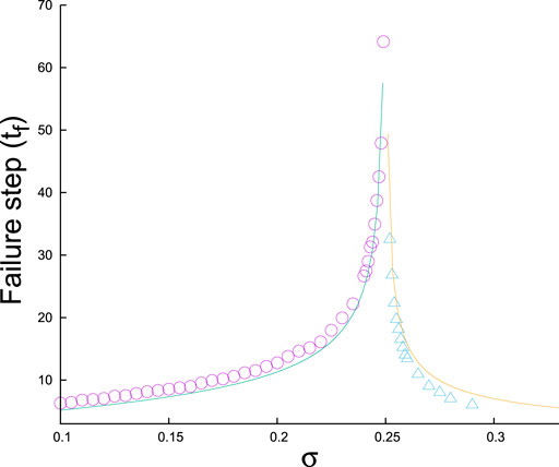
FIGURE 5. Postcritical and precritical relaxation: Numerical data are for a bundle with
The number of fibers (S) breaking between two successive stable conditions of the fiber bundle is called an avalanche. The distribution of the avalanche sizes
The load curve, in terms of the threshold values, can be written as
For the uniform threshold distribution in
The average number of fibers broken due to the increase of load from
The number of avalanches of size between S and
Therefore, the avalanche size distribution is given by
Indeed, it is possible to show 26] that for an arbitrary threshold distribution,
with
So far we have discussed the classical stress-induced failure of fibers without the presence of noise. A noise-induced failure scheme for the fiber bundle model can be formulated [13, 14, 33] for which the cooperative failure dynamics can be solved analytically.
As in the previous sections, we consider a bundle of N parallel fibers clamped between two rigid bars. A load or force
Here C is a prefactor.
Such a noise-induced failure scheme will produce two different failure regimes depending on the stress and noise levels—continuous breaking regime and intermittent breaking regime. In the continuous breaking regime, we can calculate the failure time (step) as a function of stress and noise values. However, in the intermittent breaking regime, one can define the waiting time between two consecutive failure phases.
The phase boundary can be determined through a mean-field argument that at
which finally gives
In absence of noise, when
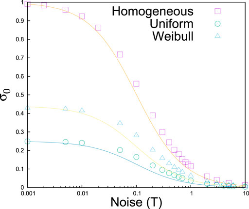
FIGURE 6. Phase boundary (
In the case of heterogeneous FBMs where fibers have different strength thresholds, keeping in mind that in absence of noise T, we should always get
The numerical data for the heterogeneous cases (Figure 6) having uniform and Weibull-type fiber strength distributions supports the conjecture well [33].
Identification of such a phase boundary has important consequences in material-fracturing and in other similar fracture-breakdown phenomena. During material/rock fracturing, acoustic emission (AE) measurements can record the burst or avalanche events in terms of AE amplitude and AE energy [34]. Therefore, AE data could reveal the correct rupture-phase of a material body under stress. Once a system enters into continuous rupture phase, the system collapse must be imminent. Thus, identification of the rupture phase can guide us to visualize the final fate of a system. It can also help to stop system collapse, if it is possible to withdraw external stress in time before the system enters into continuous rupture phase.
We will now discuss cooperative dynamics in both these regimes in the following sub-sections.
In the continuous breaking regime, one can describe the breaking dynamics in an FBM through a recursion relation [14]. Let us consider a homogeneous bundle having N fibers with exactly the same strength thresholds of 1; therefore, critical (or failure) strength of the bundle is
As all the fibers are identical,
We denote the fraction of total fibers that remain intact at time (step) t by
In the continuum limit, the above recursion relation can be presented in a differential form
Giving the failure time
The simulation result shows (Figure 7) the exact agreement with this theoretical estimate.
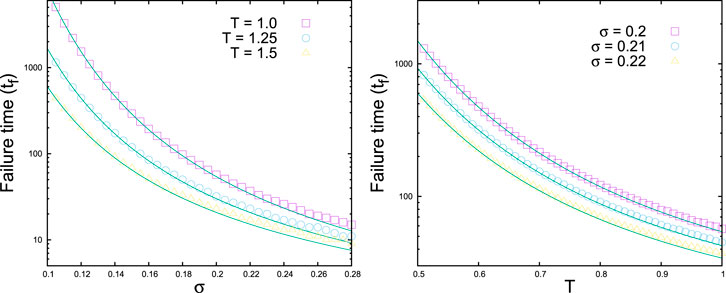
FIGURE 7. Failure time versus σ (left) and versus T (right) for a homogeneous bundle having identical fibers with a strength of 1 (
In the case of heterogeneous bundles where fibers have distributed strengths, the failure times seem to follow another form [14]:
This form was obtained through a trial and error approach. It is extremely difficult (as of now) to write the recursion relation for noise-induced failure dynamics in the case of heterogeneous systems. The simulation results have been compared with the formula above, and the agreement (Figure 8) is quite satisfactory [14].
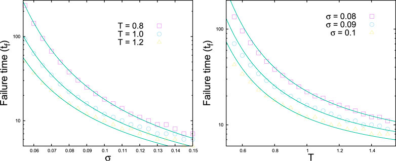
FIGURE 8. Failure time versus σ (left) and versus T (right) for bundles having uniform strength distributions. The data are for simulations over 1000 realizations with a system size of
As we discussed before, in the intermittent fracturing phase, simultaneous breaking events (avalanches) are separated by waiting times
where
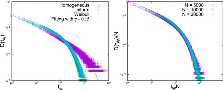
FIGURE 9. Left: The simulation results for the waiting time distributions for three different types of fiber strength distributions, with
In the waiting time distributions, the power law part dominates for small
Apparently, the modeling scheme for noise-induced rupture process is not limited to any particular system, rather it is a general approach and perhaps it can model more complex situations like rupture-driven earthquakes. In literature, we can find evidences of stress-localization around fracture/fault lines in an active seismic-zone. Also, there are several factors that can help rupture evolution, like friction, plasticity, fluid migration, spatial heterogeneities, chemical reactions, etc. To some extent, such stress redistribution/localization can be taken into account through a proper load sharing scheme and a noise term (T) can in principle represent the combined effect of all other factors.
To compare the waiting time results of the model system with real data, the California earthquake catalog from 1984 to 2002 [37] has been analyzed [33] to study the statistics of waiting times [38–40] between earthquake events. First, a cutoff (
with same γ (
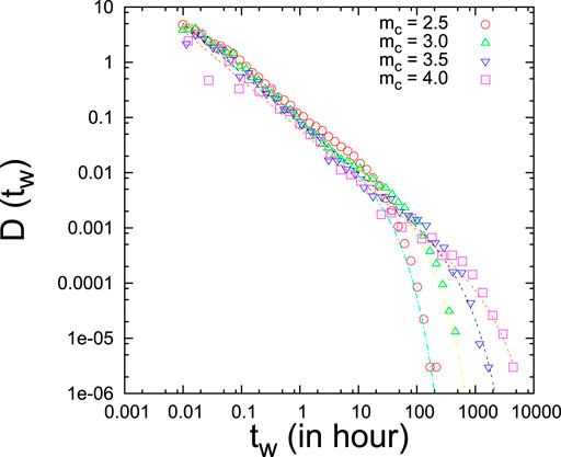
FIGURE 10. Gamma-fitting (dotted lines) to the waiting time distributions in California catalog (1984–2002).
The similarities in waiting time statistics and scaling forms suggest that slowly driven (noise-induced) fracturing process and earthquake dynamics (stick-slip mechanism) perhaps have some common origin.
So far we have considered FBM versions that are globally loaded, that is, all the fibers in the system are loaded equally from the initial time, and the load remains equal on each surviving fiber, given that the load sharing is equal. This necessarily implies that the damage or failures in the system could occur at any point; indeed, there is no notion of distance in this form of the model.
However, in fracture dynamics, particularly in the mode-1 variant of it, a front could propagate in the direction transverse to that of the loading. A fracture front necessarily implies damage localization within a region with a lower dimension than that of the system, that is, a front-line in two dimensions or a front surface in a three-dimensional system. Indeed, front propagation driven through a disordered medium is not limited to fracture; it also happens in the vortex lines in superconductors [41], magnetic domain walls in magnetic materials with impurities [42], contact line dynamics in wetting [43], and so on.
In the context of FBM, it is possible to capture the dynamics of a front propagating through a disordered medium by considering a localized loading of the system (when the fibers are arranged in a square lattice and the load is applied at an arbitrarily chosen central site; see Figure 11) in dimension higher than one (in one dimension, the damage interface is a point and hence cannot increase). The external load is increased at a low and constant rate (maintaining the separation of time scales between applied loading rate and redistribution process) [44]. Initially, the system is not loaded anywhere except for the one fiber at an arbitrarily chosen central site. As the external load increased beyond the failure threshold of the said central fiber, it breaks and the load carried by that fiber is redistributed among the fibers that are in the damage boundary (in the beginning just the four nearest neighbors). Therefore, the fibers that are newly exposed to the load after an avalanche carry a lower load compared to those accumulating loads from the earlier avalanches. This process keeps a compact structure of the cluster of the broken fibers. The localized nature of the load redistribution is justified from the fact that the newly exposed fibers are further away from the point of loading and therefore carry a smaller fraction of the load at the original central site.
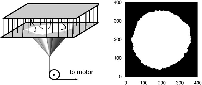
FIGURE 11. A schematic representation of locally loaded fiber bundle model and the resulting interface propagation. From [44].
As the damage perimeter increases, so does the number of fibers on that perimeter. This implies that for an avalanche, the load per fiber will decrease along the damage boundary. But due to a further increase in the load, this value will subsequently increase, initiating another avalanche. In the steady state, the load per fiber value will fluctuate around a constant and the system is said to have reached a self-organized state. In this state, the failure of fibers in the process of avalanches has a scale-free size distribution, which suggests that it is a self-organized critical (SOC) state (where external drive and dissipation balance and the critical point becomes an attractive fixed point [31]).
The steady-state value of the load per fiber and the corresponding avalanche size distribution can be calculated for a variant of this model where the load redistribution is uniform along the entire damage boundary, that is, every fiber along the damage boundary gets the same fraction of load in a redistribution process. We discuss this for the Weibull distribution below, but this is true for other distributions as well.
The Weibull distribution in its general form can be written as
where α and β are the two parameters. We can consider the particular case when
Similarly, the probability that the load is lower than x is proportional to x. Using the form for threshold distribution
Both of these functions are in good agreement with numerical simulations. Also, the saturation value of the average load per fiber can be calculated as
which is again in good agreement with simulations.
The size distribution of avalanches is a power law with the exponent value close to
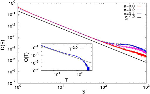
FIGURE 12. The avalanche size distributions are plotted for zero and finite lower cutoffs for Model II. The distribution function is a power law with an exponent value of
For estimating the avalanche size exponent, it can be assumed that the average load per fiber on the damage boundary has a distribution, which is Gaussian around its mean:
The probability of an avalanche being of the size between S and
By comparing Eqs. 63 and 64, we have
In this section, we would like to bring attention to some related works on the dynamics of FBM which, we believe, may be regarded as essential reading in this field.
As we have discussed in detail in the earlier sections, there has been considerable progress in characterizing the failure dynamics in the fiber bundle model through tools describing critical phenomena. One crucial step toward that direction is to identify the universality class of the model. That often needs a coarse grained description of the model, writing down the free energy form suited for the dynamics and then identifying the symmetries and consequently the universality class. One such step was done in Ref. [45] by writing down a mesoscopic description of the ELS-FBM. By specifically, writing the time evolution of the order parameter
Writing in terms of the density of intact fibers n,
with
Among other attempts to relate fracture and in particular FBM dynamics with different universality classes, a relatively less explored route is that of the hydrodynamics of turbulence. The analogy between the velocity fluctuation in turbulence and surface roughness due to fracture have been explored before [47]. However, given that FBM is able to provide a reasonably consistent picture for fracture dynamics, its association with hydrodynamics of fracture is a crucial question. In Ref. [28], the relation between the Kolmogorov energy dispersion in turbulence and avalanche dynamics in the FBM was explored. Specifically, the vortex lines in a fully developed turbulence can be mapped to self-avoiding walk (SAW) picture of polymers [48]. Then, following Flory’s theory [29], the Kolmogorov energy dispersion becomes
where q is the wave number,
It may be noted that there is also a gratifying consistency in the main results discussed above. In the ELS FBM, the critical exponents β, γ and ν for the order parameter, breakdown susceptibility and correlation length respectively satisfy the Rushbrooke scaling relation (incorporating the hyperscaling relation) [50] :
Given that the fiber bundle is essentially an ensemble of discrete elements having finite failure thresholds, under the condition of conserved load, it can serve as a generic model for intermittent progress toward catastrophic failure in a wide variety of systems. Such systems can be roads carrying traffic, power grids, or redundant computer circuitry. In several of such cases, the load redistribution following the failure of an individual element (say, traffic jam along one road, failure of one power station, etc.) is controllable to some extent–a freedom lacking in the case of stressed disordered solids. Under such circumstances, it is useful to ask the question as to how the total load-carrying capacity of the system could be maximized by a suitable load redistribution rule [51].
It is rather straightforward to establish that the maximum limit of
Intuitively, it is clear that a higher share of load should be transferred to the fibers with higher capacity. Generally, it is useful to assume that the transfer rule would be of the form
The dynamics, as discussed before, depends on whether the load is applied in a discrete step or gradually. The maximization of the strength of the system would also, therefore, depend on the loading protocol. The only parameter to tune here is b. It is possible to calculate analytically that the maximum strength is indeed achieved with this redistribution rule for
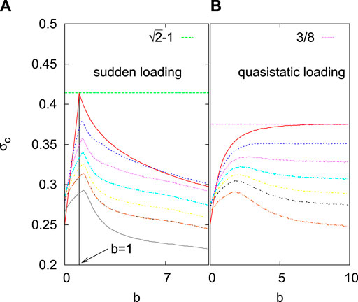
FIGURE 13. The phase diagram in the
An important information in implementing the redistribution rule is the exact knowledge of the failure thresholds of all the surviving elements. This requirement may not be always fulfilled. Assuming that there is a (fractional) error e in the knowledge of the failure thresholds, numerical simulations show (see Figure 13) that the redistribution rule still gives better results than a uniform redistribution. Therefore, in situations where the load redistribution is controllable, the redistribution rule mentioned above gives the best possible outcome.
We would like to mention that cooperative dynamics appears in another class of fiber bundle models where fibers are treated as viscoelastic elements [52–54]. The readers can go through [55] (appearing in the same research topic: The fiber bundle) for a review on viscoelastic fiber bundle models.
One can easily see that the fiber bundle model (FBM) introduced by Peirce [5] in 1926 as a model to understand the strength of composite materials is extremely elegant. As mentioned before, the model consists of a macroscopically large number of parallel fibers/springs with linear elastic behavior and of identical length. The breaking thresholds, however, are different for each fiber and are drawn from a probability distribution. All these fibers/springs hang from a rigid horizontal platform. The load on the bundle is applied at the lower horizontal platform. This lower platform has been assumed here to be rigid, implying that the stress or load share per surviving fibers/springs is equal, irrespective of how many fibers or springs might have broken (equal load sharing or ELS scheme). It may be mentioned that we have not discussed here the extensive studies on fiber bundle models with local load sharing (LLS) schemes, for which the readers may be advised to consult Refs. [1, 26], and the “impregnated fiber bundle” models for which the readers may be referred to Refs. [56, 57].
As discussed in this review, the failure dynamics of the FBM under the ELS scheme of load sharing have been analyzed for long, both analytically as well as numerically by several distinguished groups of investigators from engineering, physics, and applied mathematics. The results may be briefly summarized as follows: After introducing the model, we have described the dynamics of the equal load sharing (ELS) fiber bundle model in Section 2. Specifically, in this section, we discuss and summarize works (Refs. [1, 2, 4, 8, 28], see also [26, 40, 41]) related to the cooperative failure dynamics in the ELS fiber bundle model having a large number of fibers with different strength thresholds. We start this section by describing the force displacement relation (load curve) when the bundle is stretched by an amount x. The maximum point of this curve gives the strength of the whole bundle. One can easily derive the strength of the bundle for different fiber threshold distributions. We have chosen uniform and Weibull distributions as examples and derive bundles’ strength as critical displacement (xc) and critical force
In Section 3, we summarize some recent developments (Refs. [11–16, 47, 49, 56]) in the cooperative dynamics of noise-induced failure in ELS fiber bundle models. In addition to applied stress, the noise factor plays a crucial role in triggering the failure of individual fibers. The trick here is how to define the failure probability of individual fibers as a function of applied/effective stress and the noise level. Normally, noise-level remains constant during the entire failure process, but the stress level increases gradually due to stress redistribution mechanism. The choice of the probability function should satisfy the fact that without the noise factor the noise-induced failure model must reproduce the classical failure scenario (discussed in Section 2). We start this section by presenting a noise-induced failure probability for individual fiber failure. The choice of stress and noise level dictates whether the system is in continuous breaking regime or in intermittent breaking regime. Through a mean-field argument, one can easily find out the phase diagram separating these two regimes (Eq. 50; Figure 6). Apparently, the continuous breaking regime is easy to analyze. For a homogeneous bundle, where all the fibers are identical (strengths are the same), one can write down the failure dynamics as a recursion relation (Eq. 53). The solution gives an exact estimate for the failure time (steps) as a function of applied stress (σ) and noise level (T) (Eq. 55). Simulation results show perfect agreement with the theoretical estimates (Figure 7). When we consider a strength distribution among the fibers in the model, it becomes extremely difficult to construct the recursion relation for the failure dynamics. One reason could be that during the failure process the strength distribution gets changed with time. However, the simulation results (Figure 8) for the failure time of heterogeneous bundles follow similar variation with applied stress and noise level with an extra noise factor (Eq. 56). Next, we discuss the other regime, that is, the intermittent failure regime where there is waiting time between the two failure phases. The distribution of the waiting time is the most important aspect in this regime. Simulation results on homogeneous and heterogeneous bundles show that the waiting time distribution follows a Gamma distribution (Eq. 57) and a data collapse confirms the universal nature of such distribution function (Figure 9). Surprisingly, waiting time distribution from earthquake time series (California catalog) seems to follow a similar Gamma distribution (Figure 10).
In Section 4, we have considered self-organized fracture front propagation in a fiber bundle model where the fracture front adjusts its size in a self-organized way to meet the increasing load on the bundle and several features of the self-organized dynamics can still be analyzed in a mean field way; see, for example, Figure 12 for the avalanche size distribution, which fits well with
As already mentioned (in Section 2), the universality class of the dynamics of fixed load increment during the ongoing dynamics of failure in the bundle (until its complete failure) will be different from that for the quasi-static (or weakest link failure type) loading during its dynamics. And, as discussed in Section 5, it is given by the Flory statistics for linear polymers, when fracture dynamics in the bundle is mapped to turbulence and one utilizes the Kolmogorov-type dispersion energy cascades [28]. In particular, we already obtained ([3]; see Eqs. 35 and 36) the order parameter exponent,
As discussed in this review, the absence of stress concentrations or fluctuations around the broken fibers allows mean-field-type statistical analysis in such equal load sharing fiber bundle models. This feature of the models helped major analytical studies for the breaking dynamics and also allowed precise comparisons with computer simulation results.
BKC made the initial plan for the review article. All the authors contributed equally in discussions and in the writing of the manuscript.
This work was partly supported by the Research Council of Norway through its Centers of Excellence funding scheme, project number 262644.
The authors declare that the research was conducted in the absence of any commercial or financial relationships that could be construed as a potential conflict of interest.
BKC is grateful to J. C. Bose Fellowship Grant for support.
1. Pradhan S, Hansen A, Chakrabarti BK. Failure processes in elastic fiber bundles. Rev Mod Phys (2010) 82:499. doi:10.1103/RevModPhys.82.499
2. Pradhan S, Chakrabarti BK. Precursors of catastrophe in the Bak-Tang-Wiesenfeld, Manna, and random-fiber-bundle models of failure. Phys Rev E-Stat Nonlinear Soft Matter Phys (2002) 65:016113. doi:10.1103/PhysRevE.65.016113
3. Pradhan S, Bhattacharyya P, Chakrabarti BK. Dynamic critical behavior of failure and plastic deformation in the random fiber bundle model. Phys Rev E-Stat Nonlinear Soft Matter Phys (2002) 66:016116. doi:10.1103/PhysRevE.66.016116
4. Bhattacharyya P, Pradhan S, Chakrabarti BK. Phase transition in fiber bundle models with recursive dynamics. Phys Rev E-Stat Nonlinear Soft Matter Phys (2003) 67:046122. doi:10.1103/PhysRevE.67.046122
5. Peirce FT. Tensile tests for cottom yarns. “The weakest link” theorems on the strength of long and composite specimens. J Text Ind (1926) 17:355. doi:10.1080/19447027.1926.10599953
6. Hemmer PC, Hansen A. The distribution of simultaneous fiber failures in fiber bundles. ASME J Appl Mech (1992) 59:909. doi:10.1115/1.2894060
7. Pradhan S, Hansen A, Hemmer PC. Crossover behavior in burst avalanches: signature of imminent failure. Phys Rev Lett (2005) 95:125501. doi:10.1103/PhysRevLett.95.125501 |
8. Pradhan S, Hemmer PC. Relaxation dynamics in strained fiber bundles. Phys Rev E-Stat Nonlinear Soft Matter Phys (2007) 75:056112. doi:10.1103/PhysRevE.75.056112
9. Divakaran U, Dutta A. Effect of discontinuity in the threshold distribution on the critical behavior of a random fiber bundle. Phys Rev E-Stat Nonlinear Soft Matter Phys (2007) 75:011117. doi:10.1103/PhysRevE.75.011117
10. Lawn BR. Fracture of brittle solids. Cambridge, United Kingdom: Cambridge University Press (1993).
11. Coleman BD. Statistics and time dependence of mechanical breakdown in fibers. J Appl Phys (1958) 29:968. doi:10.1063/1.1723343
12. Scorretti R, Guarino A, Ciliberto S. Disorder enhances the effects of thermal noise in the fiber bundle model. Europhys Lett (2001) 55:626. doi:10.1209/epl/i2001-00462-x
13. Roux S. Thermally activated breakdown in the fiber-bundle model. Phys Rev E (2000) 62:6164. doi:10.1103/physreve.62.6164
14. Pradhan S, Chakrabarti BK. Failure due to fatigue in fiber bundles and solids. Phys Rev E - Stat Nonlinear Soft Matter Phys (2003) 67:046124. doi:10.1103/PhysRevE.67.046124
15. Reiweger I, Schweizer J, Dual J, Herrmann HJ. Modelling snow failure with a fibre bundle model. J Glaciol (2009) 55:997. doi:10.3189/002214309790794869
16. Cohen D, Lehmann P, Or D. Fiber bundle model for multiscale modeling of hydromechanical triggering of shallow landslides. Water Resour Res (2009) 45:W10436. doi:10.1029/2009WR007889
17. Pollen N, Simon A. Estimating the mechanical effects of riparian vegetation on stream bank stability using a fiber bundle model. Water Resour Res (2005) 41:W07025. doi:10.1029/2004WR003801
18. Pugno NM, Bosia F, Abdalrahman T. Hierarchical fiber bundle model to investigate the complex architectures of biological materials. Phys Rev E-Stat Nonlinear Soft Matter Phys (2012) 85:011903. doi:10.1103/PhysRevE.85.011903
19. Sornette D. Mean-field solution of a block-spring model of earthquakes. J Phys I France (1992) 2:2089. doi:10.1051/jp1:1992269
20. Daniels HE. The statistical theory of the strength of bundles of threads. Proc Roy Soc Ser A (1945) 183:243. doi:10.1098/rspa.1945.0011
21. Sornette D. Elasticity and failure of a set of elements loaded in parallel. J Phys Math Gen (1989) 22:L243.
23. Harlow DG, Phoenix SL. Approximations for the strength distribution and size effect in an idealized lattice model of material breakdown. J Mech Phys Solid (1991) 39:173. doi:10.1016/0022-5096(91)90002-6
24. Gómez J, Iñiguez DAF, Pacheco AF. Solvable fracture model with local load transfer. Phys Rev Lett (1993) 71:380. doi:10.1103/PhysRevLett.71.380 |
25. Hidalgo RC, Kun YF, Herrmann HJ. Fracture model with variable range of interaction. Phys Rev E - Stat Nonlinear Soft Matter Phys (2002) 65:046148. doi:10.1103/PhysRevE.65.046148
27. Pradhan S, Chakrabarti BK. Introduction to critical phenomena through the fiber bundle model of fracture. Eur J Phys (2019) 40:014004. doi:10.1088/1361-6404/aaeb53
28. Biswas S, Chakrabarti BK. Flory-like statistics of fracture in the fiber bundle model as obtained via Kolmogorov dispersion for turbulence: a conjecture. Phys Rev E (2020) 102:012113. doi:10.1103/PhysRevE.102.012113 |
30. Kolmogorov AN. Local structure of turbulence in an incompressible fluid at very high Renolds number. Dokl Akad Nauk SSSR (1941) 30:299. doi:10.1098/rspa.1991.0075
31. Biswas S, Ray P, Chakrabarti BK. Statistical physics of fracture, breakdown, and earthquake. Berlin, Germany: Wiley VCH (2015)
32. Kjellstadli JT. Burst distribution by asymptotic expansion in the equal load sharing fiber bundle model. Front Physiol (2019) 7:201. doi:10.3389/fphy.2019.00201
33. Pradhan S, Chandra A, Chakrabarti BK. Noise-induced rupture process: phase boundary and scaling of waiting time distribution. Phys Rev E - Stat Nonlinear Soft Matter Phys (2013) 88:012123. doi:10.1103/PhysRevE.88.012123
34. Petri A, Paparo G, Vespignani A, Alippi A, Costantini M. Experimental evidence for critical dynamics in microfracturing processes. Phys Rev Lett (1994) 73:3423. doi:10.1103/PhysRevLett.73.3423 |
35. Chakrabarti BK, Benguigui LG. Statistical physics of fracture and breakdown in disordered systems. Oxford, United Kingdom: Oxford University Press (1997)
36. Herrmann HJ, Roux S. Statistical models for the fracture of disordered media. Amsterdam, Netherlands: North-Holland (1990).
37.http://www.data.scec.org/ftp/catalogs/SHLK (Accessed February 1, 2005).
38. Corral A. Universal earthquake-occurrence jumps, correlations with time, and anomalous diffusion. Phys Rev Lett (2006) 97:178501. doi:10.1103/PhysRevLett.97.178501 |
39. Corral A. Local distributions and rate fluctuations in a unified scaling law for earthquakes. Phys Rev E - Stat Nonlinear Soft Matter Phys (2003) 68:035102. doi:10.1103/PhysRevE.68.035102
40. Bak P, Christensen K, Danon L, Scanlon T. Unified scaling law for earthquakes. Phys Rev Lett (2002) 88:178501. doi:10.1103/PhysRevLett.88.178501 |
41. Larkin AI, Ovchinnikov YN. Pinning in type II superconductors. J Low Temp Phys (1979) 34:409. doi:10.1007/BF00117160
42. Zapperi S, Cizeau P, Durin G, Stanley HE. Dynamics of a ferromagnetic domain wall: avalanches, depinning transition, and the Barkhausen effect. Phys Rev B (1998) 58:6353. doi:10.1103/PhysRevB.58.6353
43. Chevalier T, Talon L. Moving line model and avalanche statistics of Bingham fluid flow in porous media. Eur Phys J E Soft Matter (2015) 38:76. doi:10.1140/epje/i2015-15076-5 |
44. Biswas S, Chakrabarti BK. Self-organized dynamics in local load-sharing fiber bundle models. Phys Rev E-Stat Nonlinear Soft Matter Phys (2013) 88:042112. doi:10.1103/PhysRevE.88.042112
45. Hendrick M, Pradhan S, Hansen A. Mesoscopic description of the equal-load-sharing fiber bundle model. Phys Rev E (2018) 98:032117. doi:10.1103/PhysRevE.98.032117
46. Henkel M, Hinrichsen H, Lübeck S. Non-equilibrium phase transitions. In: Absorbing phase transitions, Vol. 1. Berlin, Germany: Springer (2008).
47. Basu A, Chakrabarti BK. Hydrodynamic descriptions for surface roughness in fracture front propagation. Philos Trans A Math Phys Eng Sci (2018) 377:20170387. doi:10.1098/rsta.2017.0387 |
48. Huang K. Lectures on statistical physics and protein folding. Singapore: World Scientific (2005).
49. Sinha S, Kjellstadli JT, Hansen A. Local load-sharing fiber bundle model in higher dimensions. Phys Rev E-Stat Nonlinear Soft Matter Phys (2015) 92:020401. doi:10.1103/PhysRevE.92.020401
51. Biswas S, Sen P. Maximizing the strength of fiber bundles under uniform loading. Phys Rev Lett (2015) 115:155501. doi:10.1103/PhysRevLett.115.155501 |
52. Hidalgo RC, Kun F, Herrmann HJ. Creep rupture of viscoelastic fiber bundles. Phys Rev E-Stat Nonlinear Soft Matter Phys (2002) 65:032502. doi:10.1103/PhysRevE.65.032502
53. Jagala EA. Creep rupture of materials: insights from a fiber bundle model with relaxation. Phys Rev E-Stat Nonlinear Soft Matter Phys (2011) 83:046119. doi:10.1103/PhysRevE.83.046119
54. Baxevanis T, Katsaounis T. Load capacity and rupture displacement in viscoelastic fiber bundles. Phys Rev E-Stat Nonlinear Soft Matter Phys (2007) 75:046104. doi:10.1103/PhysRevE.75.046104
55. Capelli A, Reiweger I, Schweizer J, Studying snow failure with fiber bundle models, Front Phys (2020) 8:236. doi:10.3389/fphy.2020.00236
56. Bunsell A, Gorbatikh L, Morton H, Pimenta S, Sinclair I, Spearing M, et al. Benchmarking of strength models for unidirectional composites under longitudinal tension. Composite A: Appl Sci Manufacturing (2018) 111:138. doi:10.1016/j.compositesa.2018.03.016
57. Breite C, Melnikov A, de Morais AB, Otero F, Mesquita F, Costa J, et al. Blind benchmarking of seven longitudinal tensile failure models for two virtual unidirectional composites. Compos Sci Technol (2021) 202:108555. doi:10.1016/j.compscitech.2020.108555
58. Pradhan S, Chakrabarti BK, Hansen A. Crossover behavior in a mixed-mode fiber bundle model. Phys Rev E - Stat Nonlinear Soft Matter Phys (2005) 71:036149. doi:10.1103/PhysRevE.71.036149
59. Roy S, Ray P. Critical behavior in fiber bundle model: a study on brittle to quasi-brittle transition. Europhys Lett (2015) 112:26004. doi:10.1209/0295-5075/112/26004
60. Roy C, Kundu S, Manna SS. Scaling forms for relaxation times of the fiber bundle model. Phys Rev E-Stat Nonlinear Soft Matter Phys (2013) 87:062137. doi:10.1103/PhysRevE.87.062137
61. Chakrabarti BK. A fiber bundle model of traffic jams. Physica A (2006) 377:162–166. doi:10.1016/j.physa.2006.05.003
62. Pahwa S, Scoglio C, Scala A. Abruptness of cascade failures in power grids. Sci Rep (2014) 4:3694. doi:10.1038/srep03694 |
63. Petri A, Pontuale G. Morphology and dynamics in SOC universality classes. J Stat Mech Theor Exp (2018) 6:063201. doi:10.1088/1742-5468/aac138
64. Pradhan S, Hansen A, Ray P. A renormalization group procedure for fiber bundle models. Front Physiol (2018) 6:65. doi:10.3389/fphy.2018.00065
Keywords: fiber bundle model, dynamic cooperation, fixed-point solution, Universality, noise-induced failure dynamics, self-organization
Citation: Chakrabarti BK, Biswas S and Pradhan S (2021) Cooperative Dynamics in the Fiber Bundle Model. Front. Phys. 8:613392. doi: 10.3389/fphy.2020.613392
Received: 02 October 2020; Accepted: 23 December 2020;
Published: 15 February 2021.
Edited by:
Subhrangshu Sekhar Manna, S.N. Bose National Centre for Basic Sciences, IndiaReviewed by:
Ferenc Kun, University of Debrecen, HungaryCopyright © 2021 Chakrabarti, Biswas and Pradhan. This is an open-access article distributed under the terms of the Creative Commons Attribution License (CC BY). The use, distribution or reproduction in other forums is permitted, provided the original author(s) and the copyright owner(s) are credited and that the original publication in this journal is cited, in accordance with accepted academic practice. No use, distribution or reproduction is permitted which does not comply with these terms.
*Correspondence: Srutarshi Pradhan, c3J1dGFyc2hpLnByYWRoYW5AbnRudS5ubw==
Disclaimer: All claims expressed in this article are solely those of the authors and do not necessarily represent those of their affiliated organizations, or those of the publisher, the editors and the reviewers. Any product that may be evaluated in this article or claim that may be made by its manufacturer is not guaranteed or endorsed by the publisher.
Research integrity at Frontiers

Learn more about the work of our research integrity team to safeguard the quality of each article we publish.