Machine learning-based analysis of sea fog’s spatial and temporal impact on near-miss ship collisions using remote sensing and AIS data

Sea fog is a severe marine environmental disaster that significantly threatens the safety of maritime transportation. It is a major environmental factor contributing to ship collisions. The Himawari-8 satellite’s remote sensing capabilities effectively bridge the spatial and temporal gaps in data from traditional meteorological stations for sea fog detection. Therefore, the study of the influence of sea fog on ship collisions becomes feasible and is highly significant. To investigate the spatial and temporal effects of sea fog on vessel near-miss collisions, this paper proposes a general-purpose framework for analyzing the spatial and temporal correlations between satellite-derived large-scale sea fog using a machine learning model and the near-miss collisions detected by the automatic identification system through the Vessel Conflict Ranking Operator. First, sea fog-sensitive bands from the Himawari-8 satellite, combined with the Normalized Difference Snow Index (NDSI), are chosen as features, and an SVM model is employed for sea fog detection. Second, the geographically weighted regression model investigates spatial variations in the correlation between sea fog and near-miss collisions. Third, we perform the analysis for monthly time series data to investigate the within-year seasonal dynamics and fluctuations. The proposed framework is implemented in a case study using the Bohai Sea as an example. It shows that in large harbor areas with high ship density (such as Tangshan Port and Tianjin Port), sea fog contributes significantly to near-miss collisions, with local regression coefficients greater than 0.4. While its impact is less severe in the central Bohai Sea due to the open waters. Temporally, the contribution of sea fog to near-miss collisions is more pronounced in fall and winter, while it is lowest in summer. This study sheds light on how the spatial and temporal patterns of sea fog, derived from satellite remote sensing data, contribute to the risk of near-miss collisions, which may help in navigational decisions to reduce the risk of ship collisions.

1 Introduction

Sea fog is a frequent and dangerous meteorological phenomenon, significantly threatening marine activity safety. This phenomenon drastically reduces the horizontal visibility of the sea surface to less than one kilometer (Gultepe et al., 2007). Unlike land-based scenarios, reduced visibility at sea poses a heightened risk due to the intricate nature of maritime navigation (Sim and Im, 2023), substantially increasing the likelihood of ship collisions and thus endangering lives, property, and the environment. Ship collisions, as one of the primary maritime accidents, can inflict substantial eco-nomic losses and adverse social impacts. Using non-accident information to understand maritime transportation safety is an effective strategy. This often involves identifying near-miss collision events from Automatic Identification System (AIS) data. Since near-miss collisions occur more frequently than actual accidents, near-miss collisions can provide richer insights for maritime traffic risk analysis than actual accident data (Zhou et al., 2021). Due to sea fog on 22 May 1922, the Peninsular & Oriental Steam Navigation Company’s Egypt collided with the French cargo ship Seine en route from London to Bombay, India. The ship sank, killing 86 passengers and crew members. Because sea fog occurs geographically heterogeneously and temporally seasonally, it is crucial to analyze how it affects near-miss collisions over time and space.

In 2000, the International Maritime Organization (IMO) adopted a new requirement for all ships to carry an Automatic Identification System (AIS) that automatically communicates information among ships and coastal authorities. The AIS system transmits the ship’s static, dynamic, and voyage information to the surrounding ships and AIS base stations via a specific Very High Frequency (VHF). Because of the rich positional and temporal information provided by AIS, it has become a valuable tool in maritime studies, including maritime traffic (Harun-Al-Rashid et al., 2022; Yang et al., 2024; Zhang et al., 2019), marine observing (Almunia et al., 2021; Wright et al., 2019), and ship collisions (Cai et al., 2021; Liu et al., 2023; Zhang et al., 2016), etc. The AIS is popular because of its ability to conduct in-depth studies of ship near-miss collisions.

Nowadays, water traffic safety studies are focusing on incidents narrowly susceptible to collisions, often termed “near-miss collisions”. In the maritime sector, a near-miss collision refers to a scenario where two vessels pass each other in close proximity (Du et al., 2020). A prevalent method for detecting near-miss collisions involves using navigation information from AIS data (Zhang et al., 2015, 2016). The few maritime accidents so far limit the possibility of conducting large-scale collision studies. However, near-miss collisions studies can help overcome this limitation (Prastyasari and Shinoda, 2020). To prevent ship collisions more effectively, numerous studies have been conducted on the spatial geographic distribution of near-miss collisions to identify high-risk areas (Du et al., 2021; Zhixiang et al., 2019; Zhou et al., 2021). However, previous studies have primarily focused on visualizing the spatial distribution of near-miss collisions without delving deeply into the relevant influencing factors. From the maritime traffic safety perspective, the factors contributing to collisions can be categorized into human, vessel, and environment domains. Among these, environmental factors are the primary causes of accidents (Zhang and Hu, 2009). Variations in environmental conditions can significantly increase collision risks. Given that marine environmental factors exhibit stability, regularity, and spatial heterogeneity, it is crucial to optimally use the rich geographic information associated with near-miss collisions. Integrating these marine environmental factors into the research framework for near-miss collisions would enable more comprehensive and insightful studies.

Among various marine environmental factors, sea fog is a frequently occurring catastrophic weather. Studies have shown that poor visibility, often associated with fog, exerts the most significant impact on maritime traffic safety, predisposing vessels to collision accidents (Bye and Aalberg, 2018; Gultepe et al., 2006). Approximately 70% of ship collisions are attributed to foggy conditions (Wu et al., 2015). Moreover, the consequences of ship collisions are most severe during the foggy season (Zhang and Hu, 2009). Investigating the influence of sea fog on near-miss collision risk is essential for enhancing the supervision and management of critical maritime areas and periods to ensure secured marine navigation.

Traditional sea fog detection methods rely on meteorological stations and buoys, which are sparse in spatial and temporal distributions (Kim et al., 2020). In recent years, remote sensing technology has been widely applied in ocean environment monitoring (Ullah et al., 2024; Khan et al., 2023). And, the advent of satellite remote sensing technology enables long-term and large-scale sea fog detection results. Using remote sensing for sea fog detection started in the 1970s when Hunt (Hunt, 1973) discovered significant differences in brightness temperatures between the mid-infrared (MIR) channel of 3.7 μm and the thermal infrared (TIR) channel of 11 μm for low clouds or fog with small particle size. Based on this theory, several studies have explored sea fog detection techniques, leveraging the difference between mid-infrared and thermal infrared channels (Cermak, 2012; Eyre et al., 1984; Wu and Li, 2014; Yibo et al., 2016; Zhang and Yi, 2013). Also, the sea fog detection accuracy can be enhanced with spectral indices, such as Normalized Snow Deposition Index, NDSI (Ryu and Hong, 2020), Normalized Difference Water Index, NDWI (Wu and Li, 2014), and Normalized Difference Flow Index, NDFI (Shi et al., 2023) and environmental factors such as air–sea temperature difference (Han et al., 2022). Due to the challenges of determining optimal thresholds with traditional methods, various machine-learning techniques are also widely employed in sea fog detection. With its unique vertically resolved measurement capability that provides accurate sea surface cloud information, the Cloud-Aerosol Lidar and Infrared Pathfinder Satellite Observation (Calipso) has been widely used for sea fog detection (Badarinath et al., 2009; Cermak, 2012; Wu et al., 2015; Xiao et al., 2023; Xiaofei et al., 2021). Sea fog based on remote sensing satellites can conduct spatial analyses of ship near-miss collisions.

Many studies have examined ship near-miss collisions to achieve a safe and reliable maritime transportation system (Chai et al., 2017; Rawson and Brito, 2021; Szlapczynski and Szlapczynska, 2016). Most recent studies infer that sea fog positively affects collisions (Heo et al., 2014; Rømer et al., 1995). However, sea fog occurrences are spatially heterogeneous and temporally seasonal. Therefore, it is necessary to explore the impact of sea fog on near miss-collision risk in time and space. Conventional global regression analysis methods, such as least squares regression, assume independence and identical distribution of observations, rendering them unsuitable for analyzing spatially unevenly distributed data. Geographically weighted regression (GWR), a local linear regression method based on spatial variation relationships, is widely applied in various fields, such as meteorology (Li et al., 2024; Wahiduzzaman et al., 2022), ecology (Wang et al., 2021; Xiao et al., 2023), and economics (Cellmer et al., 2020; Shang and Niu, 2023). The model generates a regression equation at each local location, enabling spatial analysis of sea fog’s impact on near-miss collisions (Yongtian et al., 2023).

However, few studies have focused on the spatial and temporal variations in the relationship between ship near-miss collisions and sea fog because traditional ocean observation data are usually in point form, which limits studying the relationship between sea fog and ship near-miss collisions in terms of spatial and temporal variations. To address the issue, this paper presents a novel approach of exploring the spatial and temporal variations in the relationship between ship near-miss collisions and sea fog. The primary contribution of the paper lies in proposing a framework for measuring spatial and temporal variation in the correlations between large-scale sea fog, which is detected using satellite remote sensing data instead of traditional point-based data from meteorological stations, and near-miss collisions which are derived from AIS data by the VCRO model. The GWR model measures the spatial variation of near-miss collisions influenced by sea fog while an average coefficient analysis of monthly data is used to describe the temporal variation of those collisions. The Bohai Sea is chosen as a case study to illustrate the approach. This study provides insights into the spatial heterogeneity and intra-annual seasonal variations of near-miss collisions influenced by sea fog. The approach can support decision-making for navigation and enhance maritime safety.

2 Study area and datasets

2.1 Study area

This study selected the Bohai Sea area (37°07′~41°00′N117°35′~121°10′E) as the study area (Figure 1). This region represents the northernmost offshore area of China, surrounded by land on three sides, characterized as an almost enclosed inland sea. The Bohai Sea is particularly susceptible to sea fog. Sea fog in the Bohai Sea primarily occurs during spring and less frequently in summer. Renowned for its abundance of fisheries and mineral resources and its dense concentration of ports and harbors, the Bohai Sea emerges as one of the busiest maritime regions for shipping activities.

Figure 1

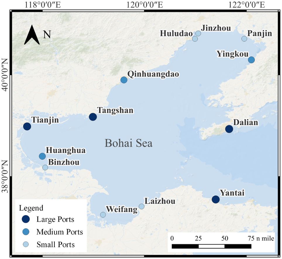
Figure 1. Overview of the study area.

In 2018, the major ports in the Bohai Sea (including Tangshan, Tianjin, Dalian, Yantai, Yingkou, and Huanghua) ranked among the world’s top 20 ports in terms of cargo throughput. The total port throughput size reflects a port’s transport capacity. According to the 2018 port data from the China Port Yearbook, the annual throughput (in million tons) of Tianjin, Tangshan, Huanghua, Qinhuangdao, Dalian, Yantai, Yingkou, Jinzhou, Huludao, Panjin, Binzhou, Dongying, Weifang, and Laizhou Ports was 507, 637, 288, 231, 468, 443, 370, 110, 31.9, 40.91, 12, 58.25, 46.57, and 22.7, respectively. The total throughput of each port is categorized into large, medium, and small sizes based on mean and standard deviation breakpoints. Large ports include Tangshan, Tianjin, Dalian, and Yantai Ports; medium ports include Yingkou, Huanghua, and Qinhuangdao Ports; and small ports include Jinzhou, Huludao, Panjin, Dongying, Binzhou, Weifang, and Laizhou Ports.

2.2 Data

2.2.1 Himawari-8

This study’s remote sensing satellite data were obtained from the Himawari-8 satellite, a third-generation geostationary meteorological satellite operated by the Japanese Meteorological Office and equipped with Advanced Himawari Imager (AHI). It covered sixteen spectral bands, including three visible light channels, three near-infrared channels, and ten infrared channels (Table 1). Its quality of cloud imagery, number of spectral bands, and clarity were substantially improved over those of previous generations. Additionally, its full-disk observation frequency of every 10 min provided excellent time resolution, thereby facilitating the study of time-series sea fog events.

Table 1

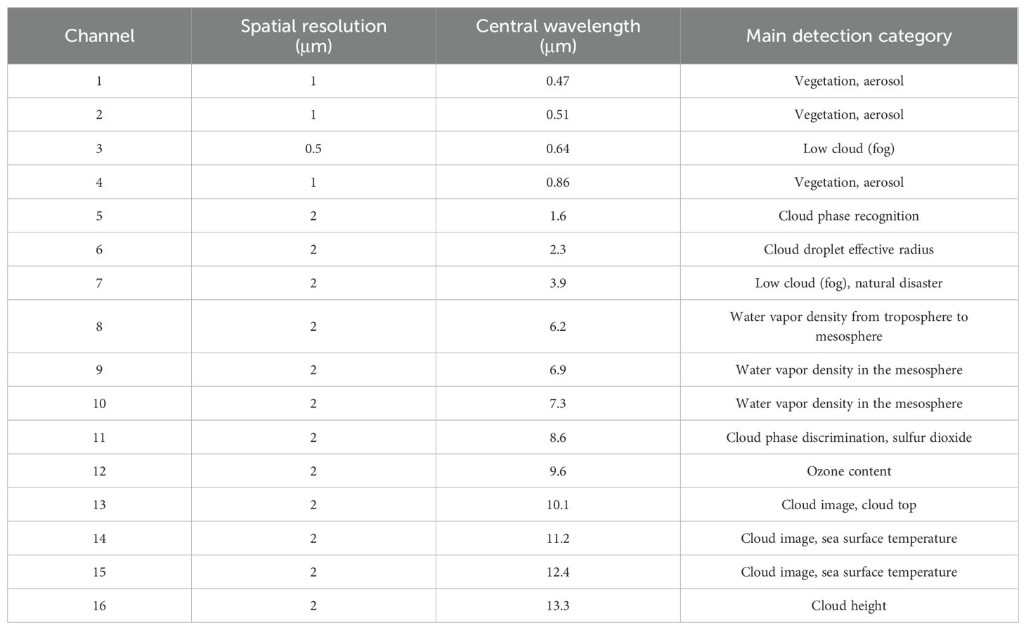
Table 1. AHI observation bands details on Himawari-8 satellite.

2.2.2 The AIS data

The Automatic Identification System (AIS) is a shipboard monitoring system that provides vital information about a ship’s position, speed, heading, and other relevant data. Being less impacted by meteorological conditions, sea surface states, and other environmental factors, AIS has gradually become a mainstream data source for ship trajectory research. The primary data used in this study is the ship’s position, timestamp, direction toward the earth, and sailing speed.

This paper used the 42.6 GB of 2018 Bohai Sea area AIS data, containing a substantial data volume. To ensure the usability of the data, we initially performed preliminary cleaning to remove records with abnormal critical information, such as speed, heading, longitude, and latitude. Since analyzing the encounter process is unpractical when the shipping speed is low or in a moored state, we filtered out low-speed data and data indicating a moored sailing state. The remaining trajectory data were then divided into several sub-trajectories for detailed analysis.

3 Methodologies

Figure 2 provides the study workflow. We explored the effect of sea fog on collision risk and the key factors influencing the collision risk as explanatory variables, such as ship density. As shown in Figure 2, the main steps include identifying sea fog, calculating collision risk, dividing the sea area to be studied into grids, counting the monthly frequency of sea fog and the total collision risk, and performing spatial analyses. The main steps are further described in detail.

Figure 2

Figure 2. Workflow of the analytical procedure.

3.1 Sea fog detection

The advantages of remote sensing satellite data include wide coverage and continuous observation, enabling constant monitoring of sea fog over a wide range and an extended period. In this study, we used Himawari-8 satellite data, which is equipped with the Advanced Himawari Imager (AHI), a next-generation sensor with 16 spectral bands ranging from visible to infrared wavelengths. The spectral characterization of Himawari-8 data identified the bands B1, B2, B3, and B14 as the most suitable for the task. To enhance the differentiation between sea fog and other features, the Normalized Snow Deposition Index (NDSI) was constructed as follows:

$\begin{array}{ll}\mathit{N}\mathit{D}\mathit{S}\mathit{I}=\frac{{\mathit{B}}_{\mathbf{3}}-{\mathit{B}}_{\mathbf{5}}}{{\mathit{B}}_{\mathbf{3}}+{\mathit{B}}_{\mathbf{5}}}& (1)\end{array}$

where B3 is the third-band reflectance and B5 is the fifth-band reflectance. Figure 3 shows the spatial distribution of NDSI index, and it can be found that most of the sea fog pixels in the Bohai Sea and Yellow Sea can be distinguished according to the NDSI index. The selected feature bands are normalized to address the varied data magnitudes in each band, which could induce low accuracy and slow computation.

Figure 3

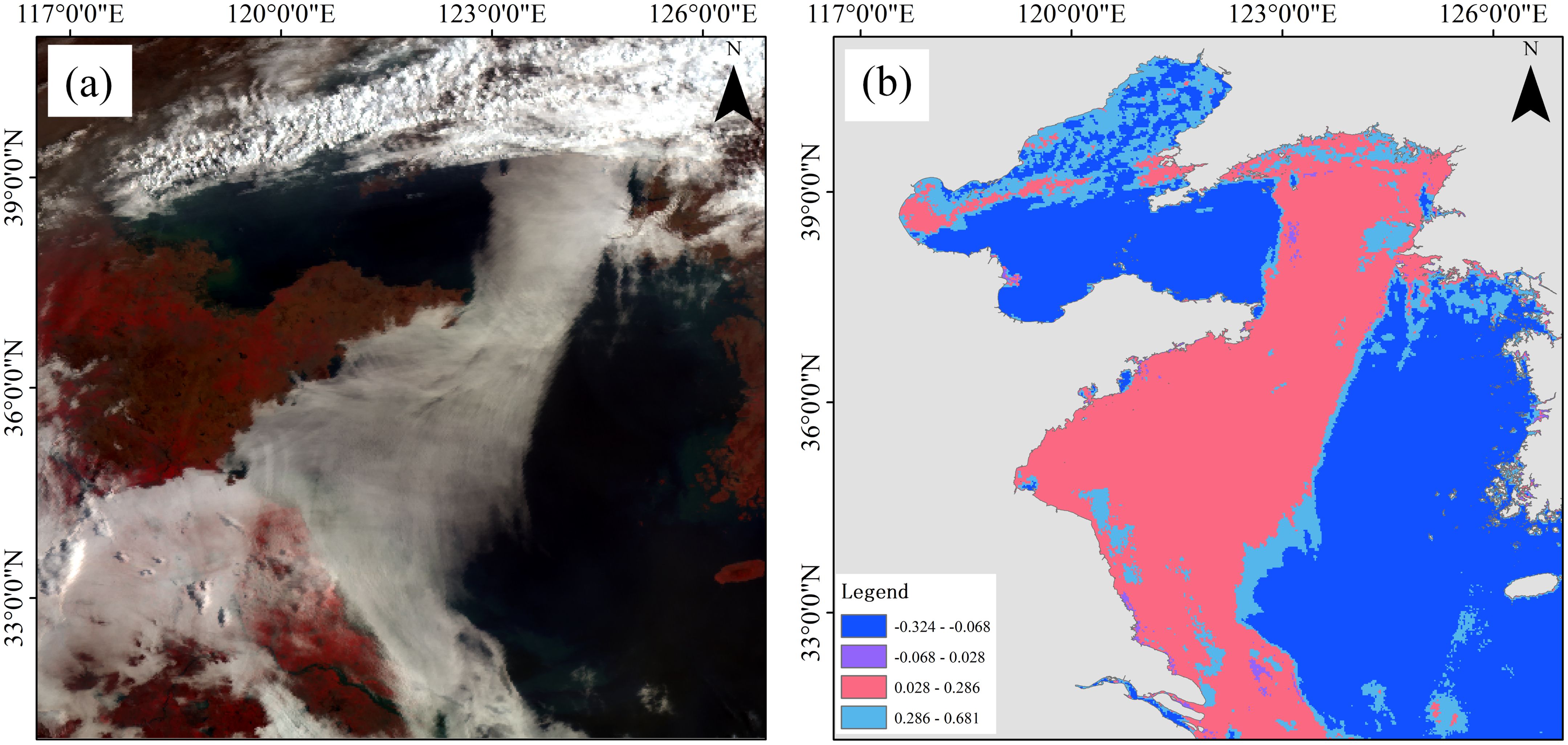
Figure 3. Himawari-8-image NDSI index distribution chart (A) Original image of Himawari-8 (B) NDSI calculation results shown in graded classes.

In this study, only sea fog is dichotomized, i.e., into fog and non-fog categories. In sea fog remote sensing detection, visual interpretation is the conventional approach to sample selection. It involves analyzing the texture or spectral characteristics of features on satellite remote sensing images to identify those that meet the pre-defined interpretation criteria. Among the visual interpretation criteria for sea fog, the following features are essential: uniform, smooth, and delicate texture, milky white color, darker and less variable brightness, and more apparent and precise boundaries. Nevertheless, low-altitude stratocumulus clouds and sea fog are essentially clouds, with no significant difference in their physical properties. Therefore, selecting sea fog samples solely based on visual interpretation of satellite remote sensing images is subjective.

Vertical Feature Mask (VFM) data, a secondary product of CALIOP data, can differentiate among several feature types, including cloud, sea surface, subsurface, stratosphere, aerosol, and no-signal data, within the range of satellite subsurface points. The data is widely used in cloud and fog detection research. Based on the CALIOP VFM data, those connected to the sea surface were considered sea fog. The synchronized transit of CALIOP VFM data and Himawari-8 satellite images are taken. Here, synchronization is a transit time difference between the two data sets of no more than 10 minutes. Samples of sea fog and non-fog conditions have been identified through visual interpretation and are further corroborated with CALIOP Vertical Feature Mask (VFM) data. Four types of feature samples, sea fog, medium-high clouds, low clouds, and sea surface, were selected through visual interpretation and in combination with CALIOP VFM data. The samples were selected by the following cases: 1) Sea fog samples are clouds in contact with the sea surface or anomalous sea surface above sea level in the VFM data. 2) Low cloud samples are clouds with cloud base heights lower than 2 km in the VFM. 3) Medium-high cloud samples are clouds with cloud base heights greater than 2 km in the VFM. The sample selection process resulted in the following types and corresponding pixel counts: 6725 pixels for sea fog, 7267 pixels for sea surface, 6961 pixels for low-level clouds, and 9367 pixels for mid-high level clouds.

The classification model in the study is the Support Vector Machine (SVM), a novel pattern recognition method initially proposed by Vapnik and Cortes in 1995 (Vapnik, 1995). The SVM is widely used in numerous domains, including feature extraction, pattern recognition, and regression analysis. Additionally, the SVM exhibits several advantageous characteristics, such as its suitability for small-sample training, robustness, stability, and automation. It has been extensively adopted, demonstrating high efficacy in remote sensing image classifications. The system randomly generates a hyperplane in the binary classification of linearly divisible data. It moves it until the points belonging to different categories in the training set are precisely on both sides of the hyperplane, thus achieving the optimal classification with the minimum difference between similar categories and vice versa. In the case of nonlinear problems, it is necessary to map the input samples to a high-dimensional feature space and construct the optimal classification surface in this feature space. As the dimensionality of the feature space increases exponentially, computing the optimal classification plane directly in this high-dimensional space becomes challenging. The SVM addresses this issue by defining a kernel function, which translates the problem to the input space. SVM can effectively divide sea fog and non-sea fog regions in high-dimensional feature space, especially suitable for complex data features in sea fog detection. SVM can accurately capture the distribution features of different regions by constructing the decision hyperplane to improve the classification accuracy. Unlike deep learning methods that usually rely on a large amount of labeled data, SVM can still provide good classification performance with limited sample size. In view of the difficulty and high cost of acquiring sea spray labeled data, CALIPSO data is used for labeling in this study, and SVM is able to give full play to its classification advantages with limited labeled samples. SVM has strong robustness to noise and outliers, which effectively improves the stability of the detection of sea spray, and reduces the classification error of the traditional methods in complex environments. Therefore, the SVM method can realize efficient processing while ensuring accuracy, and is an ideal choice for the sea fog detection task in this study.

This study selected the radial basis function (RBF) as the kernel function, with 70% of the samples used as training data and 30% as test data.

$\begin{array}{ll}\mathit{k}(\mathit{x},{\mathit{x}}^{\prime })=\mathit{\varphi }{(\mathit{x})}^{\mathit{T}}\mathit{\varphi }({\mathit{x}}^{\prime })={\displaystyle {\sum }_{\mathit{i}=\mathbf{1}}^{\mathit{M}}{\mathit{\varphi }}_{\mathit{i}}(\mathit{x}){\mathit{\varphi }}_{\mathit{i}}({\mathit{x}}^{\prime })}& (2)\end{array}$

3.2 Near miss collisions

There are two main approaches for calculating collision risk based on historical AIS data. The first method utilizes Distance at Closest Point of Approach (DCPA) and Time to Closest Point of Approach (TCPA). The technique identifies near-miss collisions by establishing criteria for DCPA and TCPA within a defined vessel domain (Fukuto and Imazu, 2013; Langard et al., 2015; Yoo, 2018). Nevertheless, collision risk assessment, solely based on DCPA/TCPA, ignores the heading information between ship pairs and thus cannot detect the collision risk during head-on encounters. The second method involves constructing a model to calculate the near-miss collisions based on factors that directly influence ship collisions.

The Vessel Conflict Ranking Operator (VCRO) model assessed the collision risks between ships, with the input variables including distance, relative speed, and phase difference between the two ships (Zhang et al., 2015). The equation is as follows:

$\begin{array}{ll}VCRO(\mathit{x},\mathit{y},\mathit{z})=((\mathit{k}{\mathit{x}}^{-\mathbf{1}}\mathit{y})(\mathit{m}·\mathbf{sin}(\mathit{z})+\mathit{n}·\mathbf{sin}(\mathbf{2}\mathit{z}))& (3)\end{array}$

where $x$ is the distance between the two ships, $y$ is the relative speed, $z$ is the phase, $k, m,n$ are the model parameters. The parameter values used in this study are based on Zhang, with k;=3.87, m=1, and n=0.386.

The relative distance between ships is calculated using Equation 4, where $(x_1,y_1)$ represents the coordinates of ship A, $(x_2,y_2)$ is the coordinates of ship B, and $d$ is the distance between the centers of the two ships.

$\begin{array}{ll}\mathit{d}=\sqrt{{({\mathit{x}}_{\mathbf{2}}-{\mathit{x}}_{\mathbf{1}})}^{\mathbf{2}}+{({\mathit{y}}_{\mathbf{2}}-{\mathit{y}}_{\mathbf{1}})}^{\mathbf{2}}}& (4)\end{array}$

The relative velocity between ships is calculated using Equation 5, where $V_a$ and $V_b$ represent the speed of ship A and ship B, respectively, $HD{G}_a$ and $HD{G}_b$ represent the heading of ship A and ship B, and $\alpha$ represents the heading angle of the ship.

$\begin{array}{ll}{\mathit{y}}_{(\mathit{a},\mathit{b})}=\sqrt{{\mathit{V}}_{\mathit{a}}^{\mathbf{2}}+{\mathit{V}}_{\mathit{b}}^{\mathbf{2}}-\mathbf{2}{\mathit{V}}_{\mathit{a}}{\mathit{V}}_{\mathit{b}}\mathbf{cos}\mathit{\alpha }}& (5)\end{array}$

The phase describes the relative position of the ships, denoted by angle and direction. The phase range is [-π, π], where a negative value indicates a concluded encounter and the two ships move away from each other, posing no collision risk. Conversely, a positive value indicates that the ships are approaching each other, heightening their collision risks.

To analyze the law governing ship collision risk on spatial and temporal scales, the study area must be gridded. Considering its size, the Bohai Sea is divided into grid cells of 0.125°, and the sum of near-miss collisions of each grid cell is counted as the value of this grid near-miss collisions:

$\begin{array}{ll}\mathit{R}\mathit{i}\mathit{s}{\mathit{k}}_{\mathit{s}\mathit{u}\mathit{m}}={{\displaystyle \sum }}^{ }\mathit{V}\mathit{C}\mathit{R}{\mathit{O}}_{\mathit{n}}& (6)\end{array}$

3.3 Global Moran’s I

Global Moran’s I is the most frequently employed statistic in global correlation analysis. It is a comprehensive measure of spatial autocorrelation across the study area (Moran, 1948). It is expressed as Equation 7, where ${\text{w}}_{\text{ij}}$ represents the weight between observations $i$ and $j$, and ${\text{S}}_0$ denotes the total sum of ${\text{w}}_{\text{ij}}$, given as Equation 8

$\begin{array}{ll}\mathit{I}=\frac{\mathit{n}}{{\mathit{S}}_{\mathbf{0}}}\times \frac{{{\displaystyle \sum }}_{\mathit{i}=\mathbf{1}}^{\mathit{n}}{{\displaystyle \sum }}_{\mathit{j}=\mathbf{1}}^{\mathit{n}}{\mathit{w}}_{\mathit{i}\mathit{j}}({\mathit{y}}_{\mathit{i}}-\overline{\mathit{y}})({\mathit{y}}_{\mathit{j}}-\overline{\mathit{y}})}{{{\displaystyle \sum }}_{\mathit{i}=\mathbf{1}}^{\mathit{n}}{({\mathit{y}}_{\mathit{i}}-\overline{\mathit{y}})}^{\mathbf{2}}}& (7)\end{array}$

$\begin{array}{ll}{\mathit{S}}_{\mathbf{0}}={\displaystyle {\sum }_{\mathit{i}=\mathbf{1}}^{\mathit{n}}{\displaystyle {\sum }_{\mathit{j}=\mathbf{1}}^{\mathit{n}}{\mathit{w}}_{\mathit{i}\mathit{j}}}}& (8)\end{array}$

A Moran’s I > 0 indicates a positive spatial correlation, described as a “high-high, low-low” aggregation trend between neighboring elements. The larger the value, the more pronounced the spatial correlation. Conversely, Moran’s I< 0 signifies a negative spatial correlation, characterized as a “high-low, low-high” distribution trend among neighboring elements. However, there is a random distribution when Moran’s I = 0, indicating spatial randomness. After calculating Moran’s I index, it is impossible to judge the spatial correlation directly based on its positive or negative value. The significance of the index must be assessed in combination with the p-value and Z-score.

3.4 Geographically weighted regression

According to the first law of geography, anything is spatially correlated. Geographically weighted regression is a local linear regression method that involves modeling spatially varying relationships to solve spatial heterogeneity of the variables by assigning weights to different locations (Brunsdon et al., 1996). Its Equation 9 is as follows:

$\begin{array}{ll}{\mathit{y}}_{\mathit{i}}={\mathit{\beta }}_{\mathbf{0}}({\mathit{\mu }}_i,{\mathit{v}}_{\mathit{i}})+{\displaystyle {\sum }_{\mathit{k}}{\mathit{\beta }}_{\mathit{k}}({\mathit{\mu }}_{\mathit{i}},{\mathit{v}}_{\mathit{i}}){\mathit{x}}_{\mathit{i}\mathit{k}}+{\mathit{ϵ}}_{\mathit{i}}}& (9)\end{array}$

where $({\mu }_i,v_i)$ denotes the position of grid cell $i$, ${\beta }_0({\mu }_i,v_i)$ is the intercept term, ${\beta }_k({\mu }_i,v_i)$ is the regression coefficient of the parameter $k$ on the grid cell, and ${ϵ}_i$ is the model random error. The parameter vector at location $i$ is estimated using the weighted least square approach as follows Equation 10:

$\begin{array}{ll}\widehat{\mathit{\beta }}({\mathit{u}}_{\mathit{i}},{\mathit{v}}_{\mathit{i}})={({\mathit{X}}^{\mathit{T}}\mathit{W}({\mathit{u}}_{\mathit{i}},{\mathit{v}}_{\mathit{i}})\mathit{X})}^{-\mathbf{1}}{\mathit{X}}^{\mathit{T}}\mathit{W}({\mathit{u}}_{\mathit{i}},{\mathit{v}}_{\mathit{i}})\mathit{y}& (10)\end{array}$

The GWR model is adjusted using a distance decay weighted function modified by a bandwidth. The three most commonly used weighting functions are Gaussian-based, bi-square, and tri-cube kernels. Bandwidth includes fixed and adaptive types. We used a geographically weighted regression model with the dependent variable as near-miss collisions, while the explanatory variables were the frequency of sea fog, ship density. We employed a Gaussian kernel spatial weight matrix, where the weight between observation points $i$ and $j$ is calculated as Equation 11, where $d_{ij}$ represents the geographical distance between the two points and $b$ is the bandwidth parameter. We used the adaptive bandwidth specified by the Akaike information criterion (AICc) due to the uneven distribution of the near-miss collision data.

$\begin{array}{ll}{\mathit{w}}_{\mathit{i}\mathit{j}}=\mathit{e}\mathit{x}\mathit{p}\left(-\frac{{\mathit{d}}_{\mathit{i}\mathit{j}}^{\mathbf{2}}}{\mathbf{2}{\mathit{b}}^{\mathbf{2}}}\right)& (11)\end{array}$

Further, the AICc and R² values evaluated the performance of the developed models. Higher R² indicates a better fit, while lower AICc indicates a poorer fit. The GWR model has significant advantages over the OLS model in its ability to optimize the global model on a local scale and to visualize the spatial distribution of the local regression coefficients. It enables the analyses of each factor’s local contribution and non-stationarity characteristics through local coefficient variations, which are unavailable in the OLS model.

4 Result and discussion

4.1 Spatial and temporal differences in near-miss collision

Figure 4 displays the grid statistics for near-miss collisions in 2018. The value for each grid represents the total values for all near-miss collisions occurring within that grid as calculated using Eq (6). Areas of high near-miss collision are concentrated around ports because of the confined navigable space and the high density of ships in these areas (Figure 5), while fewer near miss collisions were observed in the central waters of Bohai Sea. Notably, the Laotieshan Channel, located at the northernmost end of the Bohai Strait, is a major maritime transport hub in the Bohai Sea. It experiences substantial maritime traffic, resulting in a heightened risk of near-miss collision risks in the area.

Figure 4

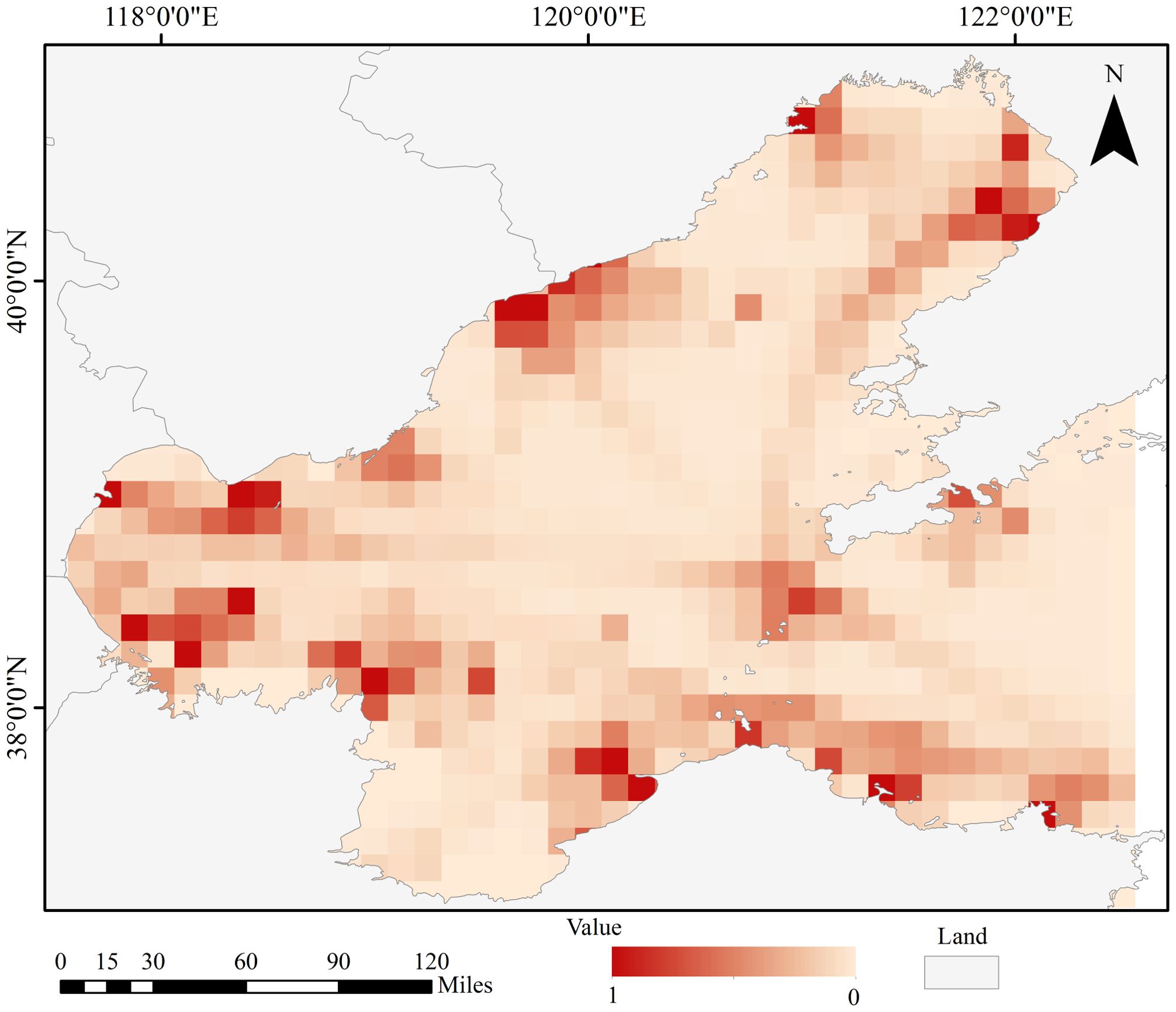
Figure 4. Spatial distribution of near-miss collisions in 2018.

Figure 5

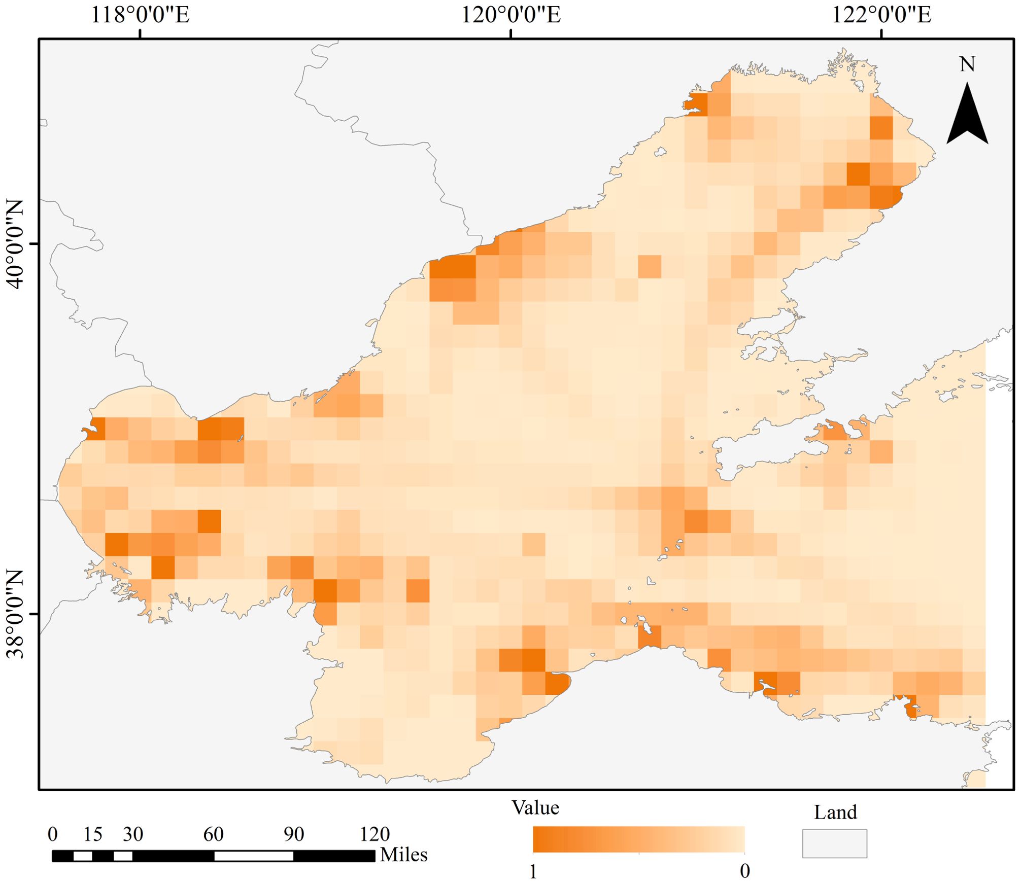
Figure 5. Spatial distribution of vessel density in 2018.

In addition, Figure 6 shows the spatial distribution of near-miss collisions from January to December 2018. We observed that the fishing moratorium in the Bohai Sea, lasting from May to August, results in fewer near-miss collisions during this period. The number of near collisions starts to increase in September. By January, vessel activity decreases as the temperature drops and the icing period begins, leading to a corresponding decline in near collisions.

Figure 6

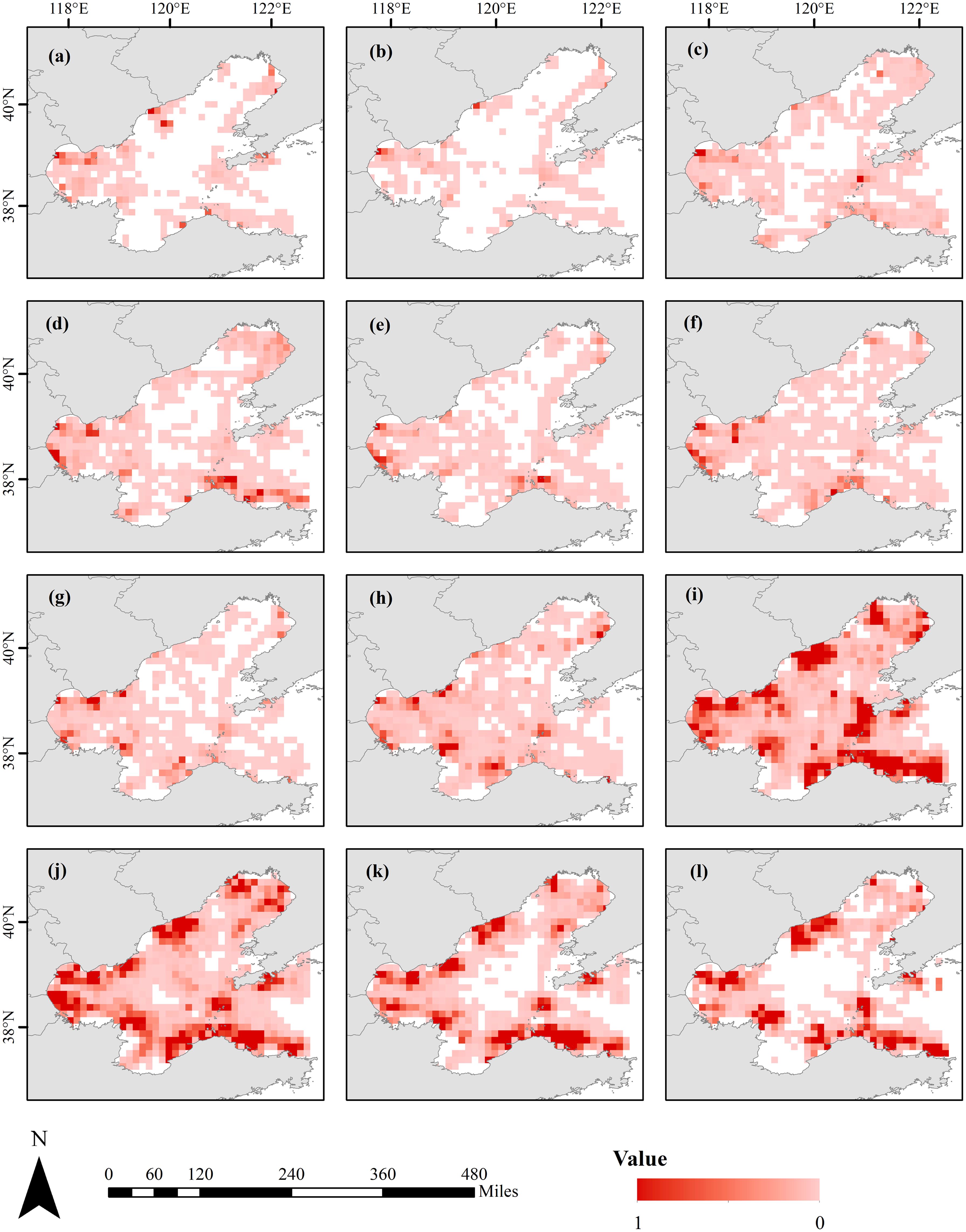
Figure 6. Spatial distribution of near-miss collisions, (A–I) represent the spatial distribution of near-miss collisions for each month from January to December 2018 respectively.

4.2 Spatial and temporal differences in sea fog

The spatial distribution of sea fog in the Bohai Sea is significantly heterogeneous, with most occurrences concentrated in the southwestern and northern regions (Figure 7).

Figure 7

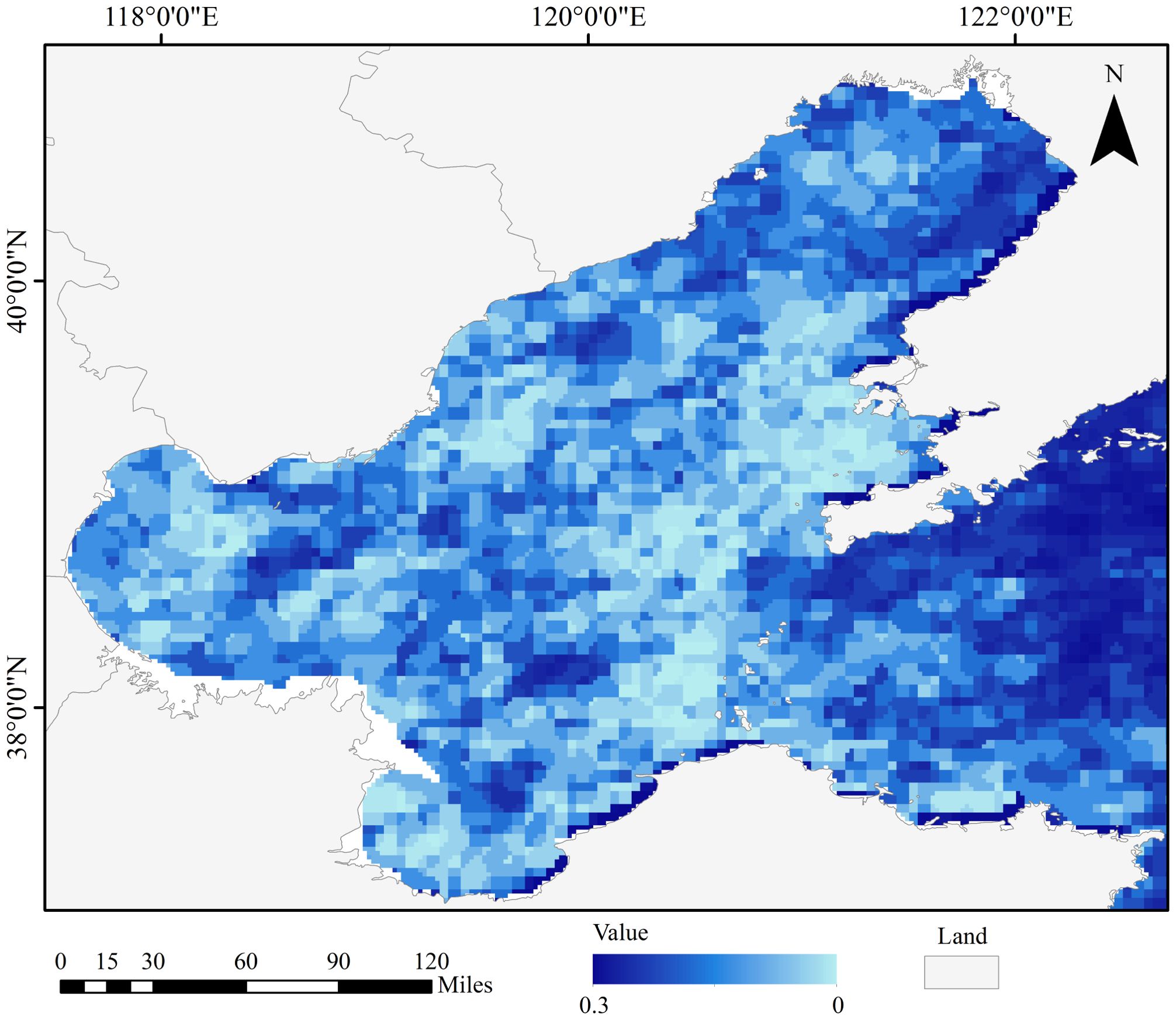
Figure 7. Spatial distribution of sea fog occurrence days in 2018.

Figure 8 illustrates the monthly distribution of sea fog frequency in the Bohai Sea in 2018. The data indicate that sea fog is significantly higher in winter and spring. Despite this seasonal peak, the overall frequency of sea fog remained relatively low, with almost no occurrences in summer.

Figure 8

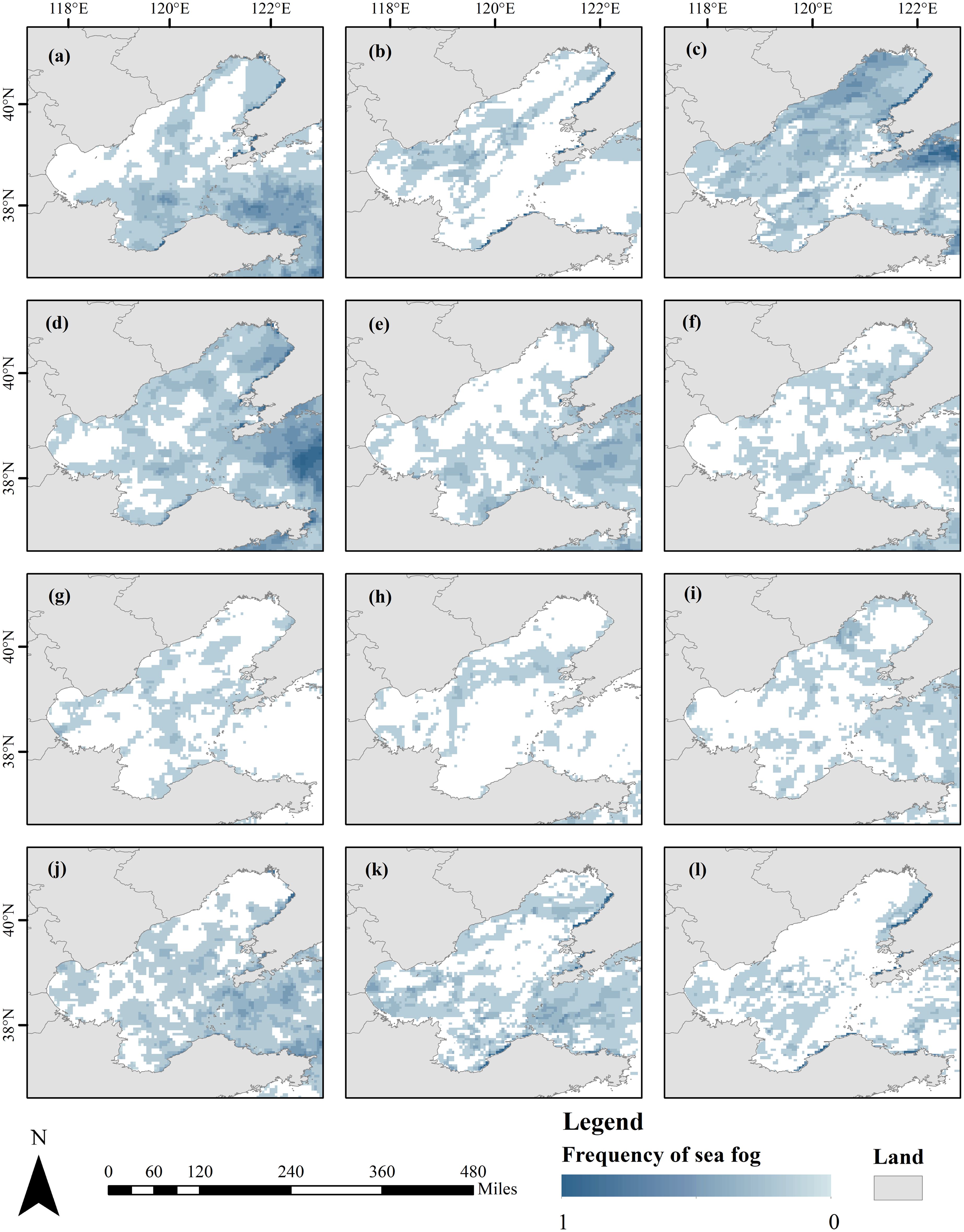
Figure 8. Spatial distribution of the frequency of sea fog occurrence, (A–I) represent the spatial distribution of the frequency of sea fog occurrence in each month from January to December 2018, respectively.

In summary, the sea fog in the Bohai Sea in 2018 has obvious spatial and temporal distribution differences, showing the characteristics of “high in spring, low in summer, high along the coast, and low in the distant sea”. Spring is the high incidence of sea fog, with a wide spatial distribution; while in summer, sea fog is significantly reduced and concentrated in local coastal areas. Understanding the spatial and temporal variability in the distribution of sea fog is critical to maritime safety and the development of effective navigation strategies.

4.3 Spatial autocorrelation

Before performing the GWR model, a spatial autocorrelation analysis of sea fog occurrence was conducted using the Moran’s I index, along with z-scores (indicating the distance from the mean in standard deviations) and p-values (assessing the statistical significance of the index). Table 2 presents these results for each month of 2018, as well as for the entire year. All the Moran’ I index values (bounded by 1.0 and 1.0) are positive and high (> 0.25), indicating a high degree of spatial positive autocorrelation. Also, the p-values are all less than 0.01 (reaching 99% confidence level), and the z-scores are significantly higher than 2.58, indicating that the spatial autocorrelation results are statistically significant. Consequently, the linear regression model is inadequate for analyzing the impact of sea fog on collision risk. In contrast, the GWR model is well-suited to address these spatial dependencies. Using the GWR model enables an in-depth analysis, better capturing the spatial impact of sea fog on near-miss collision risks across the region.

Table 2

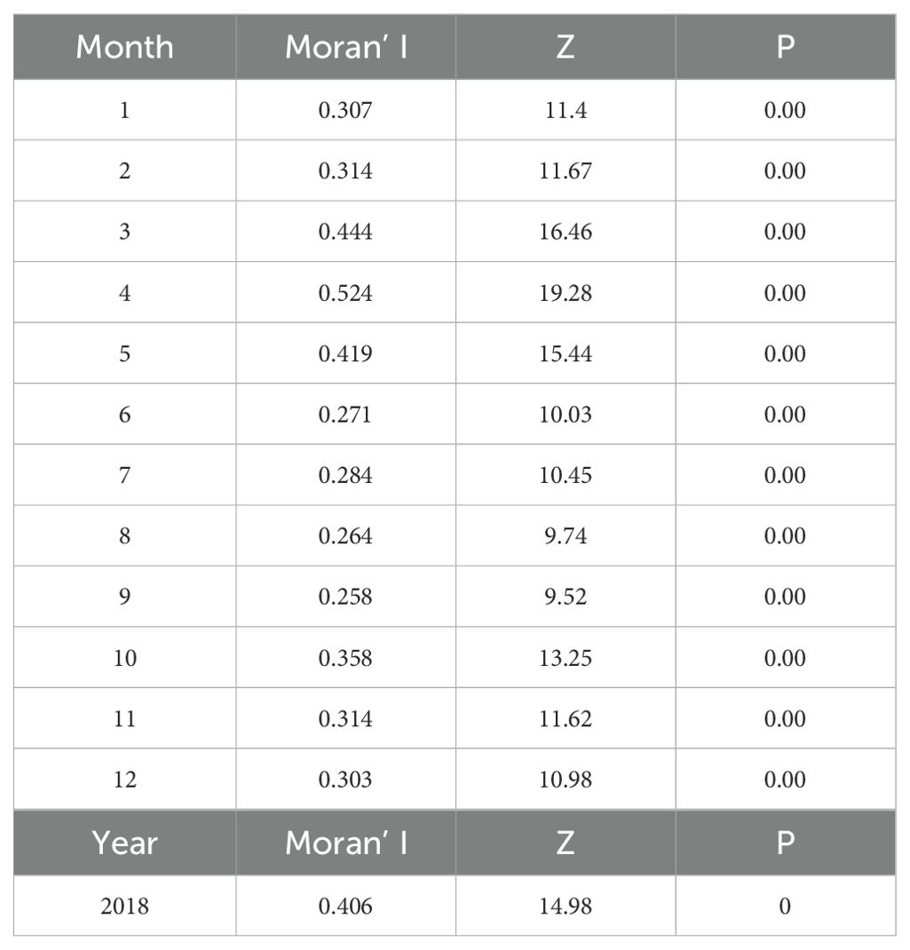
Table 2. The spatial autocorrelation test results obtained using moran’ I index combined with the z-score and p-value of sea fog (as GWR-independent variables).

4.4 GWR model diagnosis

The GWR models were constructed for 2018 and each month therein, with near-miss collisions as the dependent variable, while sea fog frequency and ship density were explanatory variables. Prior to constructing the GWR models, all values were normalized to ensure consistent scale and improve model accuracy. To assess the effectiveness of the GWR model, an OLS model was also established for comparison. The model results (Table 3) showed that the R² values of the OLS model are generally lower than 0.6, indicating that it explains less than 60% of the variance in near-miss collision incidents. For instance, in January, February, and March, the OLS R2 values are low at 0.10, 0.21, and 0.19, respectively, suggesting limited explanatory power. In contrast, the GWR model significantly outperforms the OLS model with R2 values above 0.7 for most months, indicating that its effectiveness in dealing with spatially heterogeneous data. Similarly, the Akaike Information Criterion corrected (AICc) values further validate the GWR model’s superiority. AICc is a measure of model quality where lower values indicate better fit. The AICc values of the GWR model are lower than those of the OLS model. These results indicate that the GWR model, which accounts for spatial heterogeneity, fits the data more effectively and provides more accurate regression analyses. The seasonal patterns also suggest that the GWR model performs especially well in winter and spring, when sea fog occurrences are more frequent. For example, in February through May, when sea fog events are prevalent, the GWR model R2 values range from 0.87 to 0.95. This result reinforces that sea fog, as an environmental factor, has a significant spatially variable impact on near-miss collisions during these months.

Table 3

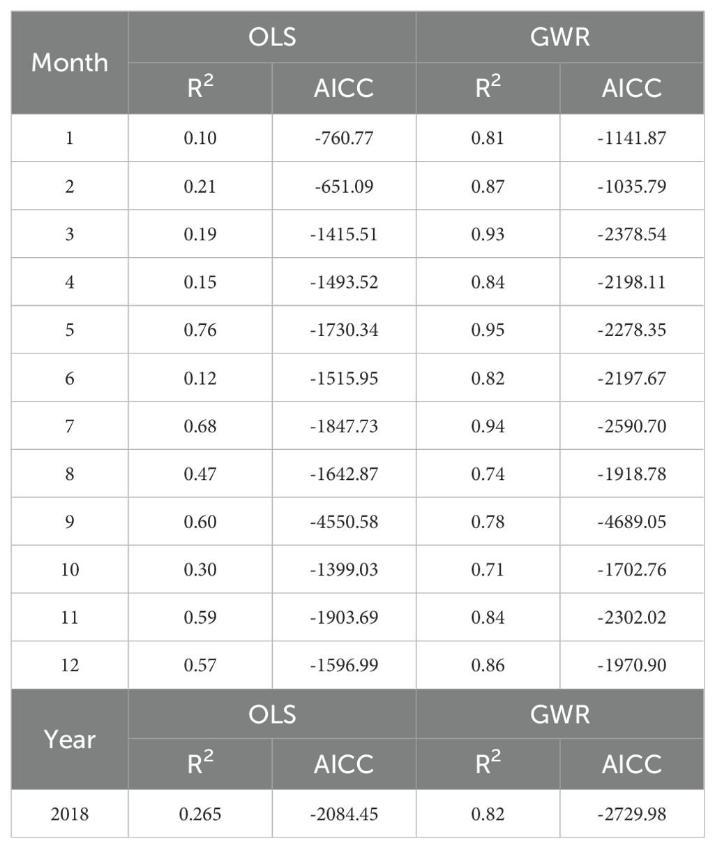
Table 3. Performance evaluation of the GWR and OLS model.

Figure 9 shows the spatial distribution of local R² values of GWR for the 2018 annual data. The values generally exceed 0.4, indicating that the sea fog and ship density can fit the GWR model well. Notably, the areas with higher R² (> 0.8) are concentrated in large port areas, such as Tianjin Port, Tangshan Port, Yantai Port, and Dalian Port. In contrast, the rest of the medium ports, such as Qinhuangdao and Yingkou Port, also have R2 between 0.6 and 0.8. Suggests that sea fog and ship density are more strongly correlated with ship near-miss collisions in ports areas.

Figure 9

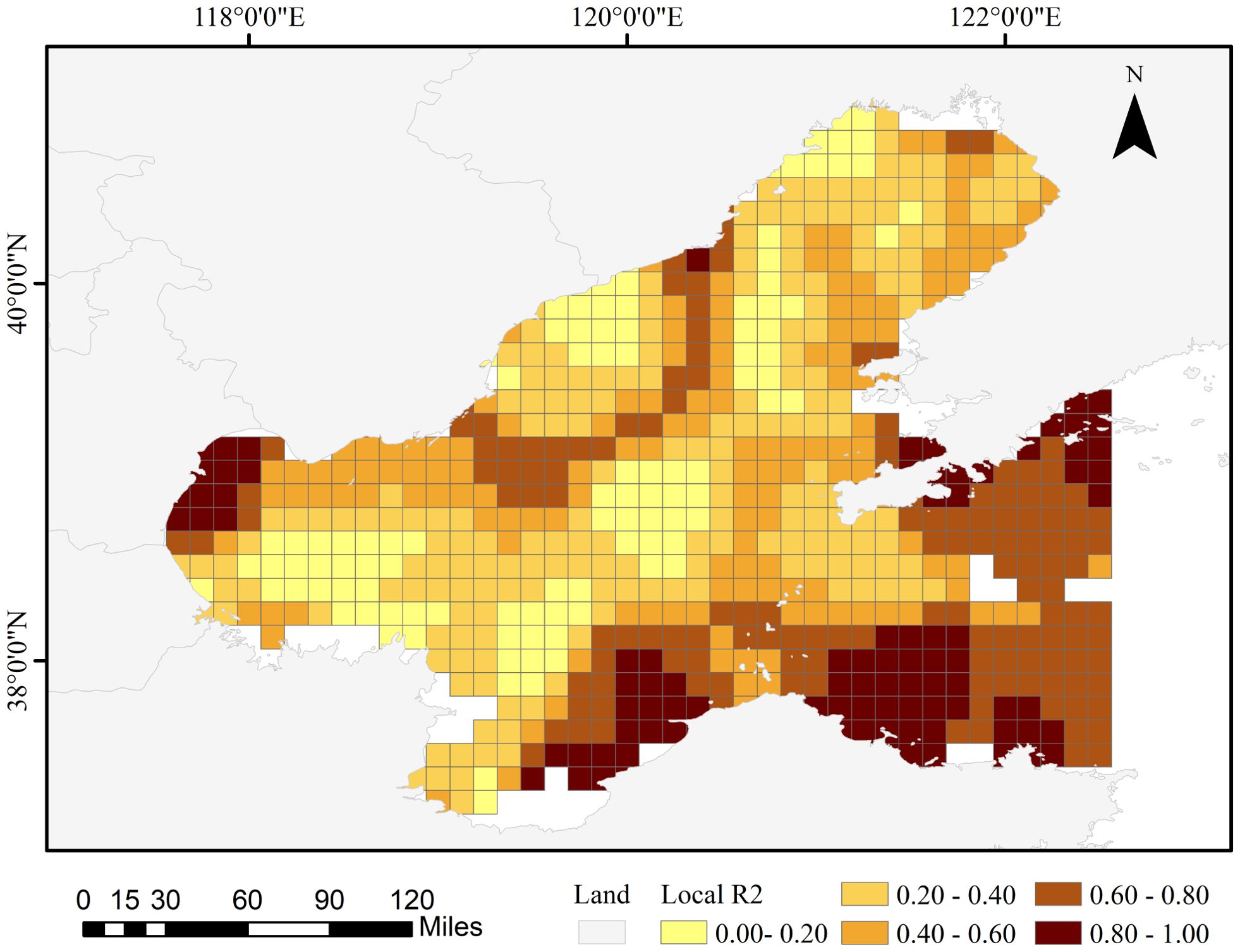
Figure 9. Spatial distribution of the local R2 values by GWR model in 2018.

Figure 10 displays the local R2 values for different locations in the GWR model over the 12 months of 2018, highlighting temporal variation in the model’s performance across different locations. The GWR model performs well in essentially all months, with local R2 values generally exceeding 0.6, although it varies monthly for different locations. This temporal variability suggests that the influence of sea fog and ship density on collision risks may shift over time, potentially due to seasonal changes in weather conditions, maritime traffic, or operational patterns in these port areas.

Figure 10

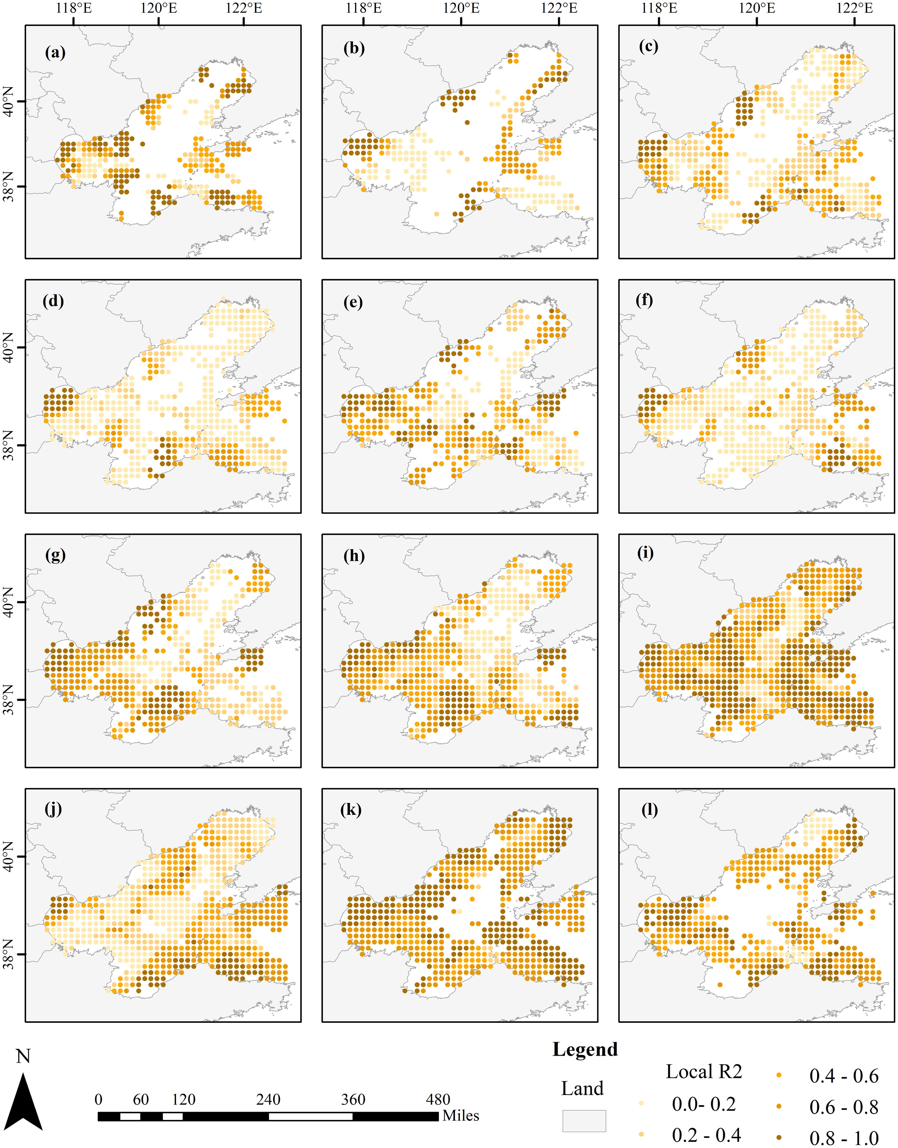
Figure 10. Spatial distribution of the local R2 values by GWR model, (A–I) represent the spatial distribution of the local R2 values in each month from January to December 2018, respectively.

Overall, the R² values are consistently high for most regions of the Bohai Sea. This deduction indicates that the driving factors used in the model effectively explain the spatial heterogeneity in near-miss collision risk.

4.5 Spatial relationship between sea fog and collision

The local regression coefficients of the GWR model (Figure 11) highlight the spatial variation in the effect of sea fog on near-miss collisions. The regression coefficients are generally greater than 0, indicating that sea fog positively affects near-miss collisions, thus the occurrence of sea fog contributing to collision risk. Generally, the impact of sea fog on near-miss collisions shows significant spatial inhomogeneity. The areas with the highest impact by sea fog are predominantly near the ports in the western part of the Bohai Sea, mainly concentrated around Tianjin Port and Tangshan Port. The high density of ships and heavy traffic in these harbors increase the likelihood of collision accidents when encountering sea fog due to reduced visibility and increased difficulty in ship handling. Further from these large ports, the coefficients decrease, indicating a relatively lower but still positive effect of sea fog on near-miss incidents. The areas with moderate coefficients (0.3 to 0.5) include regions around medium ports, where the collision risk remains elevated during fog but to a lesser extent than in the large ports. Therefore, near-miss collisions at key shipping nodes, such as ports, significantly increase during sea fog scenarios. Consequently, port authorities in large ports, such as Tianjin and Tangshan, should enhance navigation monitoring and optimize ship scheduling during foggy conditions to mitigate the increased risk of collisions. Implementing real-time navigation assistance and optimizing traffic flow in these key nodes can further reduce the risk of incidents under low-visibility conditions.

Figure 11

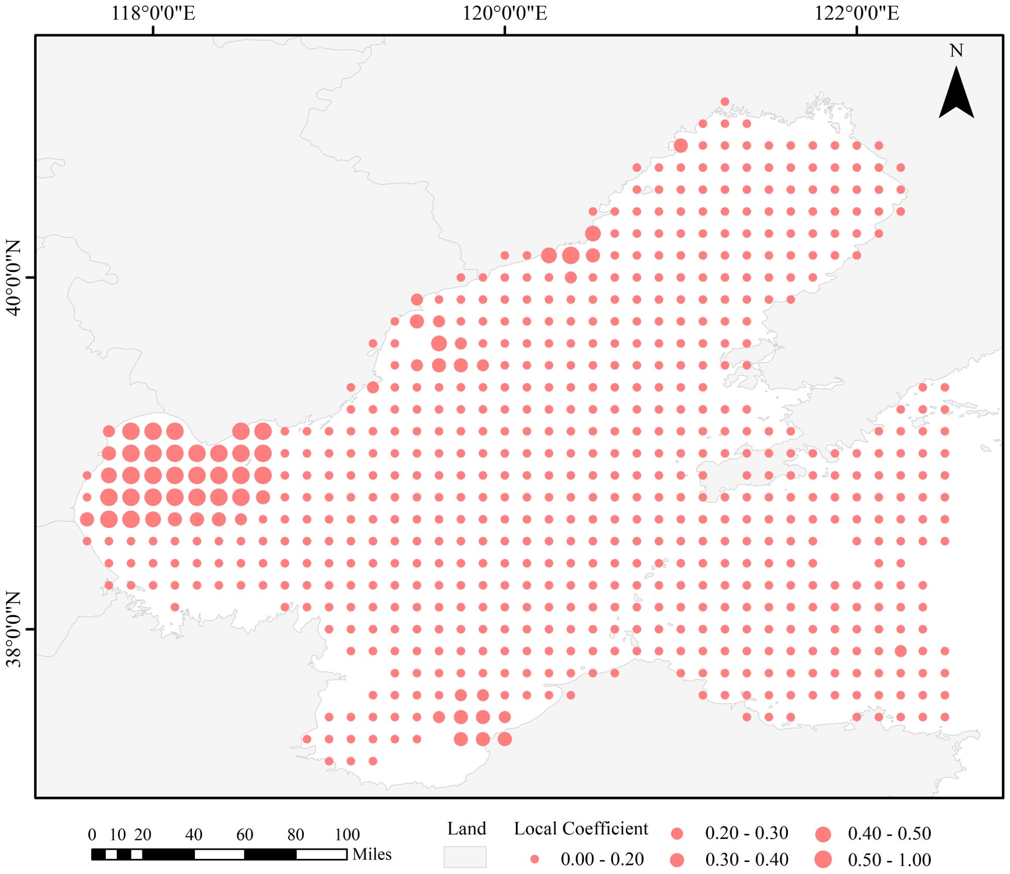
Figure 11. Spatial distribution of regression coefficient values of sea fog in 2018 using GWR models.

Figure 12 illustrates the monthly spatial distribution of local regression coefficients from the GWR model. Throughout the year, sea fog consistently shows a positive effect on near-miss collision risk, but the intensity and spatial distribution of this impact fluctuate significantly. Specifically, the contributions of sea fog were more significant in January, February, March, April, and June, with high-impact areas concentrated near the large, medium-sized ports in the western Bohai Sea, such as Tianjin and Yingkou Port. In contrast, May, July, and September display a more even distribution of lower local coefficients, with values generally below 0.1. This pattern suggests that during these months, the effect of sea fog on near-miss collisions is less severe across the region. In August, some changes occurred in the geographical distribution of the contribution of sea fog, with Dongying and Huludao harbors being more affected in localized areas. The effect of sea fog in the Bohai Sea intensified again from October to December, with several high-impact zones. Particularly in October, the effect was more significant, affecting the ports of Tianjin, Qinhuangdao, Laizhou, and Dongying. In November, Tianjin and Qinhuangdao ports were more affected, while in December, the port of Tianjin experienced the most significant impact.

Figure 12

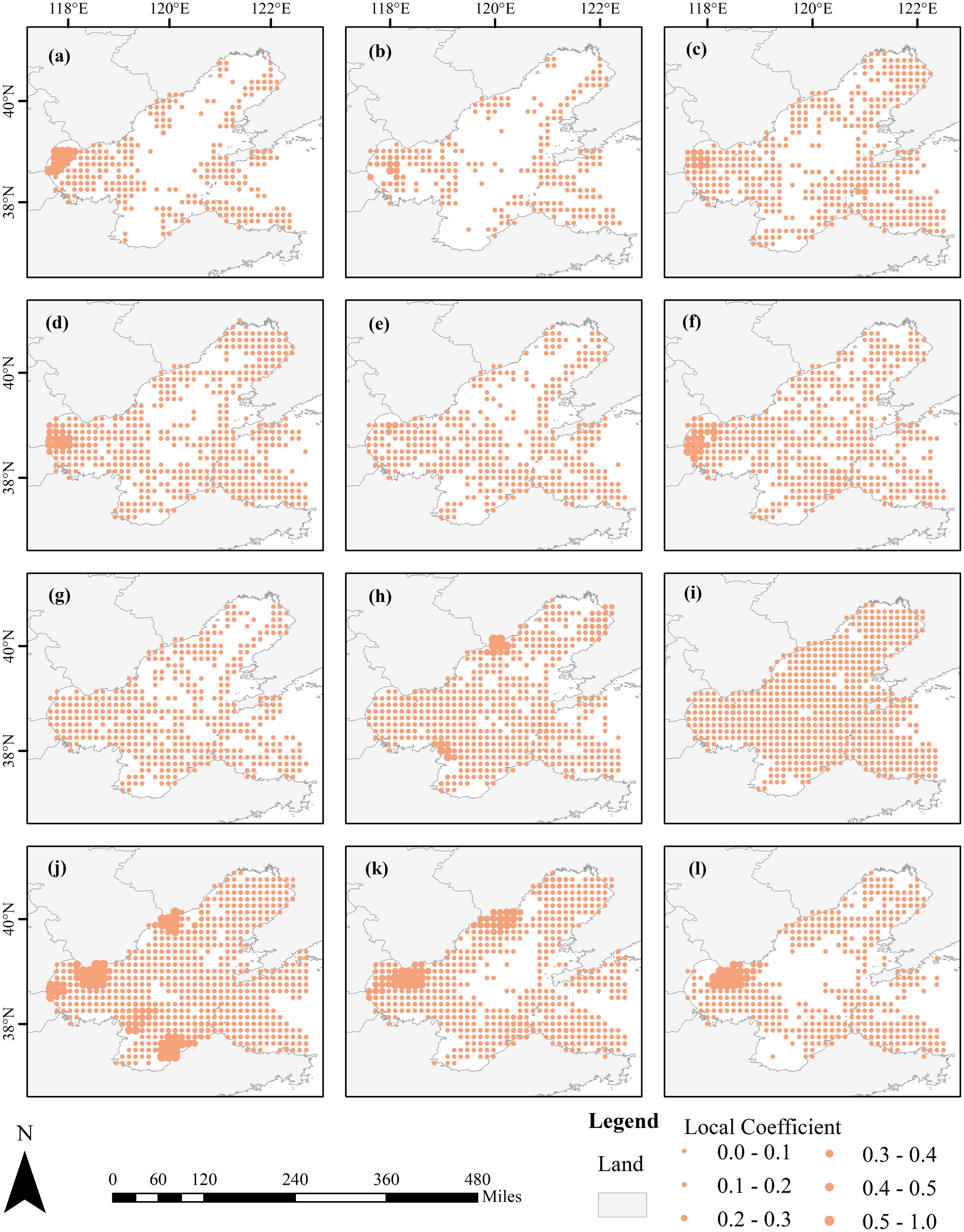
Figure 12. Spatial distribution of regression coefficient values of sea fog by GWR models, (A–I) represent the spatial distribution of regression coefficient values of sea fog in each month from January to December 2018, respectively.

4.6 Temporal relationship between sea fog and collision

Here, we present line plots of the average regression coefficients for each month in Figure 13, providing a visual comparative time-series analysis of how much the Bohai Sea area is affected by sea fog in different months. The results demonstrate that sea fog in autumn and winter most significantly impacts ships’ near-miss collisions, while spring has the second-highest impact. In contrast, the effect of sea fog on near misses is minimal in summer. The seasonal difference can be explained in two ways. First, sea fog is less frequent in summer, which directly reduces the adverse effects of sea fog on navigational conditions. Secondly, the fishing moratorium in the Bohai Sea area coincides with summer, and the reduced activity of fishing vessels leads to a relative decrease in the number of vessels, thus reducing the risk of collision due to sea fog. Nevertheless, it is crucial to note that, although May and June also fall within the fishing moratorium period, commercial vessel activity is higher at this time than from January to April. This increased activity can still contribute to collision risks, even with the reduced traffic of fishing vessels.

Figure 13

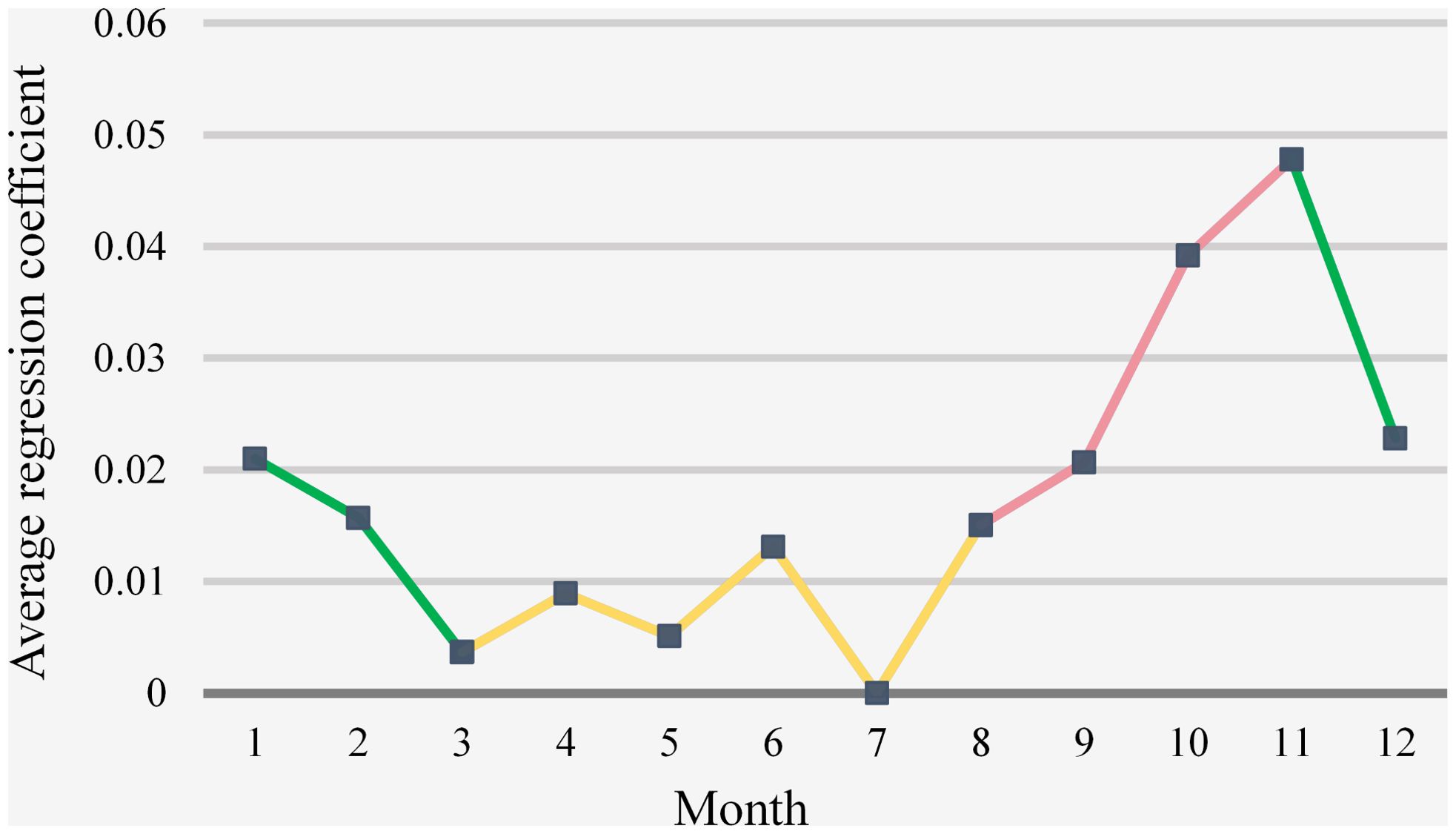
Figure 13. Average regression coefficients for January-December 2018.

Specifically, May to August is the closed season for fishing in the Bohai Sea, so the mean regression coefficient increases from September (Figure 13 red line), indicating that sea fog has started to affect ship collisions significantly. However, as winter approaches (December-March), the number of active ships decreases due to the lowering of temperatures and the freezing period, and the mean regression coefficient starts to decrease, indicating less impact by sea fog (Figure 13 green line). The regression coefficients remain smoother but slowly increase in spring and summer (March-August) (Figure 13 yellow line). In July, sea fog had almost no effect on collision risk because it hardly occurred, and the number of vessels was low during the fishing moratorium in the Bohai Sea. Collisions are more significantly affected by sea fog when vessel traffic is high. This observation suggests that navigation safety strategies should focus on periods with high vessel traffic and frequent sea fog to mitigate collision risks effectively.

5 Conclusions

This paper presents a new framework for analyzing the spatial and temporal effects of sea fog on ship near-miss collisions. Data from the Himawari-8 satellite is used to detect sea fog, with a Support Vector Machine (SVM) model applied for identification. Near-miss collisions between vessels are analyzed using the Vessel Conflict Ranking Operator (VCRO) model, which is based on Automatic Identification System (AIS) data. Spatial autocorrelation analysis by Moran ‘s I index reveals significant spatial heterogeneity in the distribution of sea fog. To account for this variability, a geographically weighted regression model (GWR) is employed, which enables measuring the spatial variation of sea fog’s effect on ship near-miss collisions through local regression coefficients. Additionally, further conduct regression analysis on the monthly time series data to investigate the intra-annual seasonal dynamics and variations by calculating the mean regression coefficients. This temporal analysis can help us understand how the sea fog factor influences ship near-miss collisions over time. The proposed framework is implemented in a case study focused on the Bohai Sea, and the results are as follows.

According to the performance metrics (AICc and R²), the GWR model performs much better than the OLS model. The R² of the GWR model ranges from 0.70 to 0.95, suggesting that GWR is more suitable for data where spatial non-stationarity exists. Regression coefficients generally greater than 0 indicate a positive influence of sea fog on ship near-miss collisions. Visualizing the local regression coefficients can intuitively reveal the spatial differences in the contribution of sea fog to ship near-miss collisions. Overall, sea areas near large and medium ports along the coast of the Bohai Sea with high ship densities, such as Tangshan Port and Tianjin Port, are more susceptible to sea fog. However, the impact on the central Bohai Sea is minimal due to the vast expanse of the water area. We estimate the mean regression coefficients for each month to explore temporal differences. It reveals that the contribution of sea fog intensifies in the autumn after the end of the fishing moratorium. In winter, the contribution of sea fog decreases due to the low number of vessel activities. However, the contribution rises steadily by spring, while it is lowest in summer due to its low occurrence frequency. Future studies should explore the spatial and temporal correlation between sea fog and ship near-miss collisions in more detail in response to multi-year data analysis. This research demonstrates that sea fog data derived from remote sensing satellite observations allows for a more comprehensive understanding of relationships and patterns in space and time.

Data availability statement

The raw data supporting the conclusions of this article will be made available by the authors, without undue reservation.

Author contributions

DL: Data curation, Software, Validation, Writing – original draft. LK: Formal Analysis, Methodology, Writing – review & editing. ZZ: Investigation, Methodology, Writing – original draft, Writing – review & editing. SZ: Methodology, Software, Validation, Writing – original draft. SL: Software, Validation, Writing – review & editing.

Funding

The author(s) declare that no financial support was received for the research, authorship, and/or publication of this article.

Conflict of interest

The authors declare that the research was conducted in the absence of any commercial or financial relationships that could be construed as a potential conflict of interest.

Generative AI statement

The author(s) declare that no Generative AI was used in the creation of this manuscript.

Publisher’s note

All claims expressed in this article are solely those of the authors and do not necessarily represent those of their affiliated organizations, or those of the publisher, the editors and the reviewers. Any product that may be evaluated in this article, or claim that may be made by its manufacturer, is not guaranteed or endorsed by the publisher.

References

Almunia J., Delponti P., Rosa F. (2021). Using automatic identification system (ais) data to estimate whale watching effort. Front. Mar. Sci. 8. doi: 10.3389/fmars.2021.635568

Crossref Full Text | Google Scholar

Badarinath K. V. S., Kharol S. K., Sharma A. R., Roy P. S. (2009). Fog over indo-gangetic plains-a study using multisatellite data and ground observations. IEEE J. Sel. Top. Appl. Earth Obs. Remote Sens. 2, 185–195. doi: 10.1109/JSTARS.2009.2019830

Crossref Full Text | Google Scholar

Brunsdon C., Fotheringham A. S., Charlton M. E. (1996). Geographically weighted regression: a method for exploring spatial nonstationarity. Geogr. Anal. 28, 281–298. doi: 10.1111/j.1538-4632.1996.tb00936.x

Crossref Full Text | Google Scholar

Bye R. J., Aalberg A. L. (2018). Maritime navigation accidents and risk indicators: an exploratory statistical analysis using ais data and accident reports. Reliab. Eng. Syst. Saf. 176, 174–186. doi: 10.1016/j.ress.2018.03.033

Crossref Full Text | Google Scholar

Cai M., Zhang J., Zhang D., Yuan X., Soares C. G. (2021). Collision risk analysis on ferry ships in Jiangsu section of the Yangtze River based on ais data. Reliab. Eng. Syst. Saf. 215, 10790. doi: 10.1016/j.ress.2021.107901

Crossref Full Text | Google Scholar

Cellmer R., Cichulska A., Belej M. (2020). Spatial analysis of housing prices and market activity with the geographically weighted regression. Isprs Int. J. Geoinf. 9, 380. doi: 10.3390/ijgi9060380

Crossref Full Text | Google Scholar

Cermak J. (2012). Low clouds and fog along the south-western African coast - satellite-based retrieval and spatial patterns. Atmos Res. 116, 15–21. doi: 10.1016/j.atmosres.2011.02.012

Crossref Full Text | Google Scholar

Chai T., Weng J., De-qi X. (2017). Development of a quantitative risk assessment model for ship collisions in fairways. Saf. Sci. 91, 71–83. doi: 10.1016/j.ssci.2016.07.018

Crossref Full Text | Google Scholar

Du L., Banda O. A. V., Goerlandt F., Kujala P., Zhang W. (2021). Improving near miss detection in maritime traffic in the northern Baltic Sea from ais data. J. Mar. Sci. Eng. 9, 180. doi: 10.3390/jmse9020180

Crossref Full Text | Google Scholar

Du L., Goerlandt F., Kujala P. (2020). Review and analysis of methods for assessing maritime waterway risk based on non-accident critical events detected from ais data. Reliab. Eng. Syst. Saf. 200, 106933. doi: 10.1016/j.ress.2020.106933

Crossref Full Text | Google Scholar

Eyre J. R., Brownscombe J. L., Allam R. J. (1984). Detection of fog at night using advanced very high resolution radiometer (avhrr) imagery. Meteorological Magazine. 113, 266–271.

Google Scholar

Fukuto J., Imazu H. (2013). New collision alarm algorithm using obstacle zone by target (ozt). IFAC Proc. Volumes 46, 91–96. doi: 10.3182/20130918-4-JP-3022.00044

Crossref Full Text | Google Scholar

Gultepe I., Mueller M. D., Boybeyi Z. (2006). A new visibility parameterization for warm-fog applications in numerical weather prediction models. J. Appl. Meteorol. Climatol. 45, 1469–1480. doi: 10.1175/JAM2423.1

Crossref Full Text | Google Scholar

Gultepe I., Tardif R., Michaelides S. C., Cermak J., Bott A., Bendix J., et al. (2007). Fog research:: a review of past achievements and future perspectives. Pure Appl. Geophys. 164, 1121–1159. doi: 10.1007/s00024-007-0211-x

Crossref Full Text | Google Scholar

Han L., Zhang S., Xu F., Lu J., Lu Z., Ye G., et al. (2022). Simulations of sea fog case impacted by air-sea interaction over South China Sea. Front. Mar. Sci. 9. doi: 10.3389/fmars.2022.1000051

Crossref Full Text | Google Scholar

Harun-Al-Rashid A., Yang C., Shin D. (2022). Detection of maritime traffic anomalies using satellite-ais and multisensory satellite imageries: application to the 2021 Suez Canal obstruction. J. Navig. 75, 1082–1099. doi: 10.1017/S0373463322000364

Crossref Full Text | Google Scholar

Heo K., Park S., Ha K., Shim J. (2014). Algorithm for sea fog monitoring with the use of information technologies. Meteorol. Appl. 21, 350–359. doi: 10.1002/met.1344

Crossref Full Text | Google Scholar

Hunt G. E. (1973). Radiative properties of terrestrial clouds at visible and infrared thermal window wavelengths 99, 346–369. doi: 10.1002/qj.49709942013

Crossref Full Text | Google Scholar

Khan S., Ullah I., Ali F., Shafiq M., Ghadi Y. Y., Kim T. (2023). Deep learning-based marine big data fusion for ocean environment monitoring: towards shape optimization and salient objects detection. Front. Mar. Sci. 9. doi: 10.3389/fmars.2022.1094915

Crossref Full Text | Google Scholar

Kim D., Park M., Park Y., Kim W. (2020). Geostationary ocean color imager (goci) marine fog detection in combination with himawari-8 based on the decision tree. Remote Sens. (Basel) 12, 149. doi: 10.3390/rs12010149

Crossref Full Text | Google Scholar

Langard B., Morel G., Chauvin C. (2015). Collision risk management in passenger transportation: a study of the conditions for success in a safe shipping company. Psychol. Fr 60, 111–127. doi: 10.1016/j.psfr.2014.11.001

Crossref Full Text | Google Scholar

Li F., Shi X., Wang S., Wang Z., de Leeuw G., Li Z., et al. (2024). An improved meteorological variables-based aerosol optical depth estimation method by combining a physical mechanism model with a two-stage model. Chemosphere 363, 142820. doi: 10.1016/j.chemosphere.2024.142820

PubMed Abstract | Crossref Full Text | Google Scholar

Liu Z., Zhang B., Zhang M., Wang H., Fu X. (2023). A quantitative method for the analysis of ship collision risk using ais data. Ocean Eng. 272, 113906. doi: 10.1016/j.oceaneng.2023.113906

Crossref Full Text | Google Scholar

Moran P. A. P. (1948). The interpretation of statistical maps. J. R. Stat. Society: Ser. B (Methodological) 10, 243–251. doi: 10.1111/j.2517-6161.1948.tb00012.x

Crossref Full Text | Google Scholar

Prastyasari F. I., Shinoda T. (2020). Near miss detection for encountering ships in sunda strait. IOP Conf. Series: Earth Environ. Sci. 557(1),12039. doi: 10.1088/1755-1315/557/1/012039

Crossref Full Text | Google Scholar

Rawson A., Brito M. (2021). A critique of the use of domain analysis for spatial collision risk assessment. Ocean Eng. 219, 108259. doi: 10.1016/j.oceaneng.2020.108259

Crossref Full Text | Google Scholar

Rømer H., Petersen H. J. S., Haastrup P. (1995). Marine accident frequencies – review and recent empirical results. J. Navig. 48, 410–424. doi: 10.1017/S037346330001290X

Crossref Full Text | Google Scholar

Ryu H., Hong S. (2020). Sea fog detection based on normalized difference snow index using advanced himawari imager observations. Remote Sens. (Basel) 12, 1521. doi: 10.3390/rs12091521

Crossref Full Text | Google Scholar

Shang X., Niu H. (2023). Analysis of the spatiotemporal evolution and driving factors of China’s digital economy development based on esda and gm-gwr model. Sustainability 15, 11970. doi: 10.3390/su151511970

Crossref Full Text | Google Scholar

Shi X., Liu X., Zhao S., Gu Y. (2023). Applicability comparison of three classical remote sensing retrieval methods for nighttime sea fog in Shandong offshore. doi: 10.1117/12.2668131

Crossref Full Text | Google Scholar

Sim S., Im J. (2023). Improved ocean–fog monitoring using himawari-8 geostationary satellite data based on machine learning with shap-based model interpretation. IEEE J. Sel. Top. Appl. Earth Obs. Remote Sens. 16, 7819–7837. doi: 10.1109/JSTARS.2023.3308041

Crossref Full Text | Google Scholar

Szlapczynski R., Szlapczynska J. (2016). An analysis of domain-based ship collision risk parameters. Ocean Eng. 126, 47–56. doi: 10.1016/j.oceaneng.2016.08.030

Crossref Full Text | Google Scholar

Ullah I., Ali F., Sharafian A., Ali A., Naeem H. M. Y., Bai X. (2024). Optimizing underwater connectivity through multi-attribute decision-making for underwater iot deployments using remote sensing technologies. Front. Mar. Sci. 11. doi: 10.3389/fmars.2024.1468481

Crossref Full Text | Google Scholar

Vapnik V. (1995). The nature of statistical learning theory (Springer, Berlin, Germany).

Google Scholar

Wahiduzzaman M., Cheung K. K., Luo J., Bhaskaran P. K. (2022). A spatial model for predicting north Indian Ocean tropical cyclone intensity: role of sea surface temperature and tropical cyclone heat potential. Weather Clim Extrem 36, 100431. doi: 10.1016/j.wace.2022.100431

Crossref Full Text | Google Scholar

Wang D., Wan R., Li Z., Zhang J., Long X., Song P., et al. (2021). The non-stationary environmental effects on spawning habitat of fish in estuaries: a case study of coilia mystus in the Yangtze estuary. Front. Mar. Sci. 8. doi: 10.3389/fmars.2021.766616

Crossref Full Text | Google Scholar

Wright D., Janzen C., Bochenek R., Austin J., Page E. (2019). Marine observing applications using ais: automatic identification system. Front. Mar. Sci. 6. doi: 10.3389/fmars.2019.00537

Crossref Full Text | Google Scholar

Wu C., Dong H., Ai W. (2015). “Security countermeasures on ships sailing in the fog,” in International Conference on Electrical Engineering and Mechanical Automation (ICEEMA 2015). USA: DEStech Publications, Inc. 341–345.

Google Scholar

Wu X., Li S. (2014). Automatic sea fog detection over Chinese adjacent oceans using terra/modis data. Int. J. Remote Sens. 35, 7430–7457. doi: 10.1080/01431161.2014.968685

Crossref Full Text | Google Scholar

Wu D., Lu B., Zhang T., Yan F. (2015). A method of detecting sea fogs using caliop data and its application to improve modis-based sea fog detection. J. Quant Spectrosc Radiat. Transf 153, 88–94. doi: 10.1016/j.jqsrt.2014.09.021

Crossref Full Text | Google Scholar

Xiao Y., Liu R., Ma Y., Cui T. (2023). Merra-2 reanalysis-aided sea fog detection based on caliop observation over north pacific. Remote Sens. Environ. 292, 113583. doi: 10.1016/j.rse.2023.113583

Crossref Full Text | Google Scholar

Xiao G., Wang T., Luo Y., Yang D. (2023). Analysis of port pollutant emission characteristics in United States based on multiscale geographically weighted regression. Front. Mar. Sci. 10. doi: 10.3389/fmars.2023.1131948

Crossref Full Text | Google Scholar

Xiaofei G., Jianhua W., Shanwei L., Mingming X., Hui S., Muhammad Y. (2021). A scse-linknet deep learning model for daytime sea fog detection. Remote Sens. (Basel) 13, 5163. doi: 10.3390/rs13245163

Crossref Full Text | Google Scholar

Yang J., Bian X., Qi Y., Wang X., Yang Z., Liu J. (2024). A spatial-temporal data mining method for the extraction of vessel traffic patterns using ais data. Ocean Eng. 293, 116454. doi: 10.1016/j.oceaneng.2023.116454

Crossref Full Text | Google Scholar

Yibo Y., Zhongfeng Q., Deyong S., Shengqiang W., Xiaoyuan Y. (2016). Daytime sea fog retrieval based on goci data: a case study over the yellow sea. Opt Express 24, 781-801. doi: 10.1364/OE.24.000787

PubMed Abstract | Crossref Full Text | Google Scholar

Yongtian S., Zhe Z., Dan L., Pei D. (2023). Exploring spatial non-stationarity of near-miss ship collisions from ais data under the influence of sea fog using geographically weighted regression: a case study in the Bohai Sea, China. Hai Yang Xue Bao 42, 77–89. doi: 10.1007/s13131-022-2137-7

Crossref Full Text | Google Scholar

Yoo S. (2018). Near-miss density map for safe navigation of ships. Ocean Eng. 163, 15–21. doi: 10.1016/j.oceaneng.2018.05.065

Crossref Full Text | Google Scholar

Zhang W. B., Goerlandt F., Kujala P., Wang Y. H. (2016). An advanced method for detecting possible near miss ship collisions from ais data. Ocean Eng. 124, 141–156. doi: 10.1016/j.oceaneng.2016.07.059

Crossref Full Text | Google Scholar

Zhang W., Goerlandt F., Montewka J., Kujala P. (2015). A method for detecting possible near miss ship collisions from ais data. Ocean Eng. 107, 60–69. doi: 10.1016/j.oceaneng.2015.07.046

Crossref Full Text | Google Scholar

Zhang J. P., Hu S. P. (2009). Application of formal safety assessment methodology on traffic risks in coastal waters & harbors. doi: 10.1109/IEEM.2009.5373103

Crossref Full Text | Google Scholar

Zhang L., Meng Q., Fang Fwa T. (2019). Big ais data based spatial-temporal analyses of ship traffic in Singapore port waters. Transportation Res. Part E: Logistics Transportation Rev. 129, 287–304. doi: 10.1016/j.tre.2017.07.011

Crossref Full Text | Google Scholar

Zhang S., Yi L. (2013). A comprehensive dynamic threshold algorithm for daytime sea fog retrieval over the Chinese adjacent seas. Pure Appl. Geophys. 170, 1931–1944. doi: 10.1007/s00024-013-0641-6

Crossref Full Text | Google Scholar

Zhixiang F., Hongchu Y., Ranxuan K., Shih-Lung S., Guojun P. (2019). Automatic identification system-based approach for assessing the near-miss collision risk dynamics of ships in ports. IEEE Trans. Intell. Transp Syst. 20, 534-543. doi: 10.1109/TITS.2018.2816122

Crossref Full Text | Google Scholar

Zhou Y., Yang J., Bian X., Ma L., Kang Z. (2021). Macroscopic collision risk model based on near miss. J. Navig. 74, 1104–1126. doi: 10.1017/S0373463321000321

Crossref Full Text | Google Scholar