 Jie Yu
 Han Zhang
 Huizan Wang3*
 Di Tian
 Jiagen Li
- 1State Key Laboratory of Satellite Ocean Environment Dynamics, Second Institute of Oceanography, Ministry of Natural Resources, Hangzhou, China
- 2Southern Marine Science and Engineering Guangdong Laboratory (Zhuhai), Zhuhai, China
- 3College of Meteorology and Oceanography, National University of Defense Technology, Changsha, China
The upper ocean structure obviously affects sea surface temperature cooling (SSTC) induced by tropical cyclones (TCs). Herein, principal component analysis of many Argo profiles from 2001 to 2017 in the Northwest Pacific Ocean is used to classify the upper ocean structure. The results suggest that the upper ocean structure can be divided into four types of water. Water with low mode 1 scores (M1-L water) is characterized by an extremely warm sea surface temperature (SST), while a cold and thick isothermal layer is observed for water with high mode 1 scores (M1-H water). Water with high mode 2 scores (M2-H water) has a warm SST and a thick isothermal layer. Relative to M2-H water, water with high mode 3 scores (M3-H water) has a warmer SST but a shallower mixed layer. These waters have remarkable seasonal and spatial variability, mainly associated with the impacts of solar radiation, precipitation, currents and mesoscale eddies. The ocean responses to TCs are different among these water types, which greatly influences the TCs intensification. The response of M1-H water is not considered, since its SST is below 26°C. The TC-induced SSTC of M3-H water (-1.12°C) is markedly higher than that of M1-L (-0.68°C) and M2-H waters (-0.41°C). Moreover, the one-dimensional mixed layer model shows a much smaller entrainment rate for M2-H water due to its thick barrier layer. The number of each water type changes in association with global warming and Kuroshio path, and thus affects the TC intensification.
1 Introduction
Tropical cyclones (TCs), characterized by strong winds and heavy rainfalls, are some of the most devastating natural disasters (Emanuel, 2005). The Northwest Pacific (NWP) is the most active basin in the world for TCs, accounting for approximately one-third of all TCs. Accurate prediction of TCs is critical for reducing casualties and property losses in many countries. Compared to the rapid development in tropical cyclone (TC) track forecasting, it has been difficult to improve TC intensity forecasting (Wang and Wu, 2004; DeMaria et al., 2014; Kossin and DeMaria, 2016).
Heat exchange at the air-sea interface plays a significant role in TC intensification, and sea surface temperature (SST) is usually used as a forecasting metric (Wu et al., 2008; Park et al., 2011; Tao and Zhang, 2014; Shay et al., 2015; Lyu et al., 2019). SST impacts TC development. Holliday and Thompson (1979) noted that a SST higher than 28°C is a critical condition for rapidly intensifying typhoons in the NWP. Generally, the intensifying rate of TCs is fastest with SSTs between 27°C and 30°C (Chan and Duan, 2001). The tropical cyclone heat potential (TCHP), measuring the upper ocean heat content from sea surface to the depth of the 26°C isotherm (), is also applied to investigate the relationship between TC intensification and ocean heat content (OHC) (Leipper and Volgenau, 1972). Upper ocean temperature generally decreases during TC passage, which greatly reduces the TCHP. Thereby the TCHP for maintaining a TC is 10-16 (Leipper and Volgenau, 1972), while it is more than 60 for TC intensification (Leipper and Volgenau, 1972; Mainelli et al., 2008). High TCHP in the NWP usually benefits TC intensification (Wada and Chan, 2008; Wada et al., 2012).
The interaction between a TC and the upper ocean layer is a two-way process. On the one hand, SST generally decreases when TCs pass through (Price, 1981; Zhang et al., 2016; Lin et al., 2017; Zhang et al., 2018; Li et al., 2020). On the other hand, sea surface temperature cooling (SSTC) reduces the air-sea difference, thus decreasing enthalpy fluxes. The upper ocean response to a TC is a negative feedback loop. TC-induced mixing is recognized to cause most of the irreversible heat flux in the mixed layer by transferring wind momentum into the upper ocean and air-sea heat exchange accounts for the remainder of flux (Price, 1981; Wang et al., 2016; Zhang et al., 2016). Moreover, TC intensity and translation speed markedly influence TC-induced mixing (Wang et al., 2016; Zhang et al., 2021).
In addition to TC characteristics, the upper ocean vertical structure also plays a key role in TC-induced mixing (Wang et al., 2011; Balaguru et al., 2012). The vertical structure in the NWP is complex and has been the focus of many studies. Previous studies have indicated that the depth of the mixed layer clearly influences the SSTC (Chan and Duan, 2001; Wu et al., 2008; Wang et al., 2016). When a TC passes through areas with shallower mixed layers, the cold sea water under the mixed layer is easier to entrain by wind forcing and upwelling. For example, He et al. (2022) investigated the SSTC difference between typical oceanic water, the Kuroshio, and warm eddies and showed that the Kuroshio and warm eddies suppressed the TC-induced SSTC more than the typical oceanic water did. Kawakami et al. (2022) also identified that thick mixed layer depth (MLD) and small temperature gradient below the MLD reduced the SSTC caused by TC-induced mixing.
Due to the halocline influence, the uniform density mixed layer becomes shallower than the uniform temperature isothermal, which means that there is important stratification in the isothermal layer (De Boyer Montégut et al., 2007). The layer between the base of the mixed layer and the base of the isothermal layer is defined as the barrier layer. Yan et al. (2017) have thoroughly researched the effects of the barrier layer on the upper ocean responses to a TC. When TC-induced entrainment cannot break through the mixed layer, the barrier layer is disadvantageous for TC development (Vincent et al., 2012). However, when TC-induced entrainment breaks through the mixed layer, the barrier layer is beneficial for TC intensification. Entraining barrier layer water, which is warmer than the cooled mixed layer, to the surface compensates for the SST, thus supporting TC intensification. Moreover, because the value of the Richardson number in the barrier layer is larger and stratification is stronger, the gravity stability is high, preventing the downward development of the ocean turbulence process.
In this paper, the relationship between TCs intensification and the upper ocean which contains thermal conditions and vertical structure in the NWP is further investigated. Thermal conditions are represented by the SST, and OHC (Potter and Rudzin, 2021). Moreover, the vertical structure is represented by the MLD, isothermal layer depth (ILD) and barrier layer thickness (BLT) (Balaguru et al., 2012; Balaguru et al., 2016; Yan et al., 2017; Potter and Rudzin, 2021). Section 2 introduces the TC best track, Argo and mesoscale eddy datasets. Section 3 describes the methods used in this study, including the oceanic metrics and statistical methods, as well as the one-dimensional mixed layer adopted here. Section 4 shows the characteristics and distributions of the upper ocean structures. The forming mechanism of the structures is discussed in this section as well. Moreover, the distribution of TCs intensification and how the upper ocean structure influences it are analyzed here. Finally, the summary and conclusions are presented in Section 5.
2 Data
The TC data used in this study are obtained from the Joint Typhoon Warning Center (JTWC, http://www.usno.navy.mil/JTWC). This dataset contains the 6-hourly central locations, intensity, maximum sustained wind speed (Vmax) and other key parameters of each tropical cyclone in the NWP from 2000 to 2020. Because sea surface temperature anomalies induced by weak TCs are not obvious and other background factors also cause similar phenomena, only strong TCs (Vmax 64 Kt) are considered in this study, and there are a total of 257 out of 477 tropical cyclones generated from 2001 to 2020 in the NWP are examined. The research region is from 10°N to 30°N and between 105°E and 140°E (red box in Figure 1A), where the TC density is high. Since the genesis time of TCs in the NWP is concentrated in the period between July and October (Figure 1B), this period is regarded as the TC season in this paper.
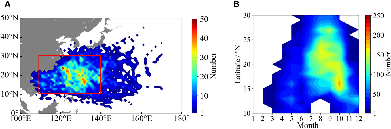
Figure 1 The spatial and temporal distribution of TC density. (A) Spatial distribution of TC density, (B) Latitude-month distribution of TC density.
The Array for Real-time Geostrophic Oceanography (Argo) program is a large-scale ocean observation plan that aims to quickly collect temperature and salinity profiles above 2000 m, which helps to greatly improve the accuracy of climate and weather prediction. To ensure the quality of the data, the global Argo scattered dataset (V3.0) obtained from the China Argo Real-time Data Center (CARDC, ftp://ftp.argo.org.cn/pub/ARGO/global/) is adopted in this study. This dataset undergoes post-quality control, including real-time quality control and a set of special tests (Liu et al., 2021). It primarily examines the observation time and position of the Argo floats. Moreover, if the float drift speed is greater than 2 m/s, the Argo float is assigned a value of “4”. Then, abnormal pressure, temperature and salinity values are checked. For instance, if the observed pressure does not uniformly increase or the observed temperature and salinity are out of normal range, the data are assigned a value of “4”. If the observed data is good after quality control, it will be assigned a value of “1”. Only Argo floats with a value “1” are selected in this study. These data contain the observation time, satellite positioning information, corrected pressures ( Pa), corrected temperature (°C), and corrected salinity (PSU).
To accurately describe the vertical structure of the upper ocean, each Argo profile is further identified using the following criteria: only profiles with (1) water depths greater than 300 m and (2) a minimum observation depth shallower than 10 m are considered. In total, 43048 Argo profiles between 2001 and 2022 that satisfy these criteria are used here (Figure 2).

Figure 2 Distribution of Argo profiles. The number of Argo points is in a grid box (black contours of 100, 150, 200, 250) during 2001-2022.
Mesoscale eddies, known as main ocean features, are abundant in the NWP. To investigate the temporal and spatial distribution of mesoscale eddies in the NWP, a global Lagrangian eddy dataset (GLED v1.0, https://zenodo.org/record/7349753#.ZD-LHexBxz8; Liu and Abernathey, 2023) based on the satellite altimetry product from Earth System Science Data was used in this study. This dataset divides the eddies into 30-day, 90-day and 180-day eddies based on their lifespans. Moreover, it contains the central position, equivalent radius and trajectory over the lifetime of each eddy.
3 Methods
3.1 Ocean metrics
For each Argo profile, the following variables were calculated: SST, MLD, ILD, BLT, , OHC and TCHP. SST is considered as the temperature at the shallowest observation depth. and represent the temperature and density at 10 m, respectively, in the Argo profile data. Since most Argo initial observation depths are less than 10 m and the ILD and MLD are generally deeper than 10 m in the NWP, the ILD is defined as the depth where the temperature is 0.5°C less than . The MLD is considered the depth with a density difference of from . The difference between the ILD and MLD is the BLT. The equation for is:
where represents the salinity at 10 m.
The equations for OHC and TCHP are:
where is the specific heat of water at a constant pressure and and are the temperature and density at the ith level, respectively. is the thickness of the ith level.
3.2 Statistical method
To reduce the data complexity, principal component analysis (PCA) is used here to reduce the dimensionality of abundant data, as shown in the Figure 3. In this research, a sample matrix including the MLD, ILD, BLT, SST, , and OHC data is created, and the Z score (Zero-mean normalization) is chosen to standardize these data so that each variable has a mean of 0 and a variance of 1 (, , , , , ). The covariance matrix is to measure the relationships of these ocean matrices, since there is a certain correlation between each ocean metric. Moreover, calculating the covariance matrix is a key procedure in PCA. Because the dataset involves six variables (, , , , , ), the shape of this covariance matrix is . The eigenvectors of the covariance matrix form the principal component matrix and are also the new, uncorrelated modes that are linear combinations of the standardized variables. Only the first k () modes with large variance (,…, ) values are retained, while the other modes with nearly 0 variance are ignored. The first k modes (,…, ) can provide a reasonable explanation for the patterns and physical background. Since the cumulative variance contribution of the first k modes reaches a high level, it is possible to use fewer than six new modes to illustrate significant patterns.
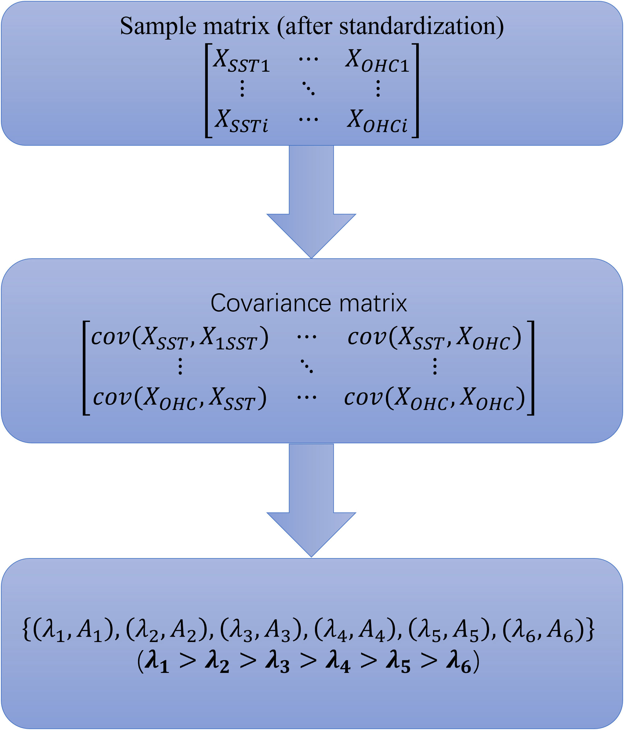
Figure 3 Schematic diagram of PCA calculation.
3.3 One-dimensional mixed layer model
The one-dimensional Price-Well-Pinkel (1DPWP; Price et al., 1986) model is adopted here to investigate the thermodynamical response of the upper ocean, focusing on the different structures. The sea surface heat flux and precipitation are set as 0 in this model, and only the wind stress is considered in this model. The gradient Richardson numbers and critical bulk values are set as 0.25 and 0.65, respectively.
The wind stress is calculated by the following equation:
where is the air density, is the drag coefficient, and is the maximum wind speed obtained from the JTWC dataset. According to Powell et al. (2003) and Shay et al. (2015), the value of is calculated through the following equation:
4 Results
4.1 Characteristics of different structures
The eigenvalues for the six modes are 118725, 100390, 24566, 6423, 8181, and 0. Since the eigenvalues of the first three modes contribute to more than 94% of the sum of all the eigenvalues in the data (mode 1: 46%, mode 2: 39%, mode 3: 10%), only the first three modes are considered in this paper (Figure 4). Linear combinations of the standardized variables for the first three modes are shown in the following equations:
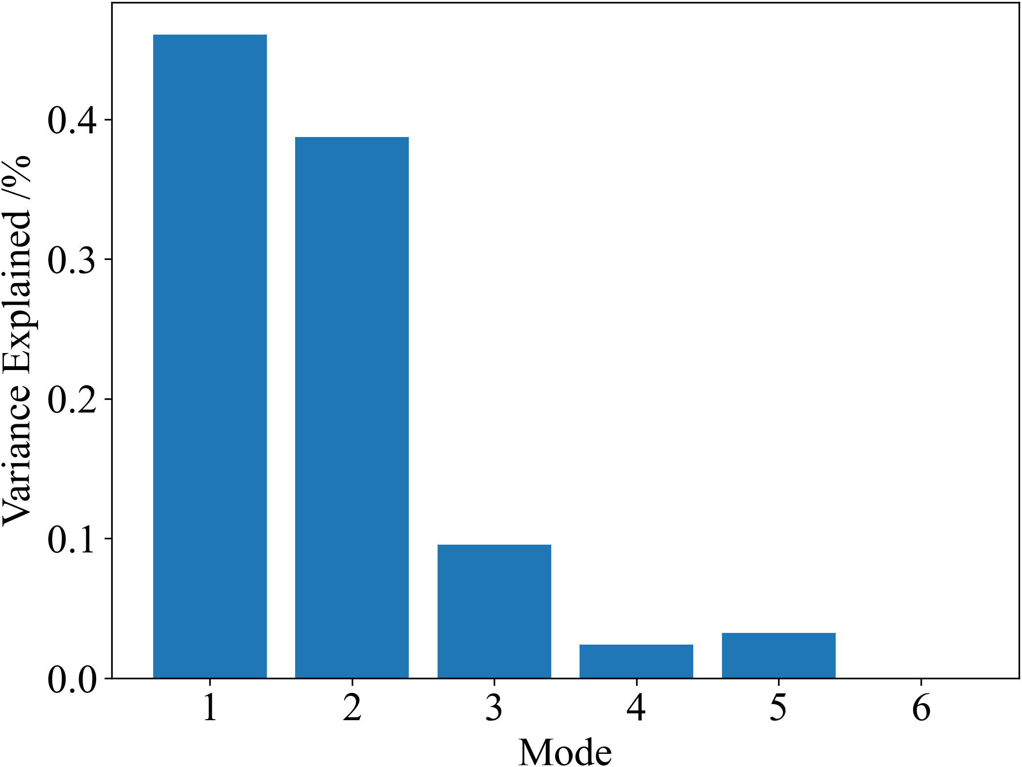
Figure 4 Bar chart showing the percentage of variance in the data that is explained by each of the six modes.
Applying these standardized variable data to the equations, mode scores for each profile are calculated and the loading for each variable determines its contribution. Moreover, a significance test is performed on the modes. The results show that modes 1, 2 and 3 significantly differ (p 0.05) every month.
Since the loadings of SST, and OHC are all negative, mode 1 OHC has a reciprocal relationship with SST and , and all of them decrease the mode 1 score. In contrast, the ILD and BLT both markedly increase the mode 1 score. Therefore, a low mode 1 score represents a structure with high SST, high OHC and deep (Figure 5A). The high mode 1 score shows a structure with low OHC, deep ILD and thick BLT (Figure 5B). Unlike mode 1, mode 2 dominantly describes that OHC has a strong relationship with other variables except SST which plays little or no role in increasing the mode 2 score. Profiles with a high mode 2 score have a relatively warm SST, large OHC, and thick MLD, ILD and BLT values (Figure 5C) due to their positive loadings. For mode 3, an MLD with a large positive coefficient greatly decreases the mode score. Therefore, an observation with a high mode 3 score generally has an extremely shallow MLD, high OHC, warm SST, and relatively thick ILD, BLT and values (Figure 5D).
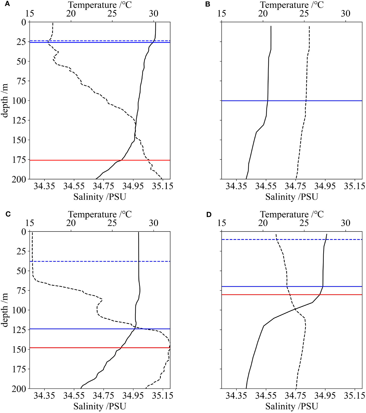
Figure 5 Examples of temperature profiles with low mode 1, high mode 1, high mode 2, and high mode 3 (A-D). The black solid lines represent temperature and black dashed lines represent salinity. The blue solid lines indicate the ILD, blue dashed lines indicate the MLD, and red solid lines indicate the depths of the 26°C isotherm.
Profiles with low mode 1, high mode 1, high mode 2, and high mode 3 scores are hereafter called M1-L, M1-H, M2-H, M3-H water, respectively. There are obvious difference among the averaged metrics of these water (Table 1). Notably, the MLD calculation of the M1-H water is not sensitive to the density threshold value. Hence, the ILD of the M1-H water is regarded as the MLD. M1-L water has the highest SST and the shallowest BLT. M1-H water has the lowest SST. M2-H water has the thickest ILD, BLT and . M3-H water has the shallowest ILD and MLD.
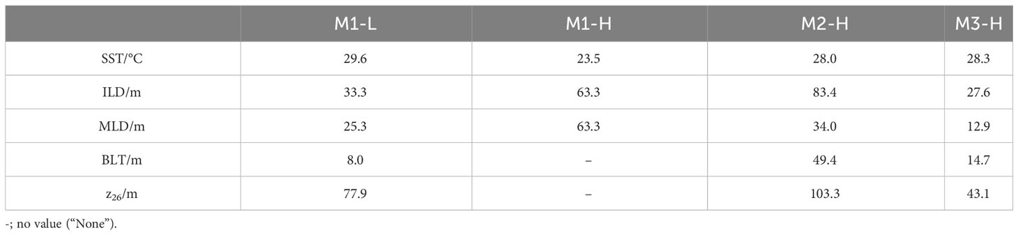
Table 1 The averaged metrics of different waters.
Waters with a TCHP greater than 60 in the TC season are further analyzed (Mainelli et al., 2008), as shown in Table 2. Because the TCHP of the M1-H water is 0, Table 2 does not show the results for M1-H water. The number of M1-L water bodies with TCHP ≥ 60 reaches a minimum in January and a maximum in September. The average TCHP of the M1-L water reaches a maximum in May (Table 2). The M2-H water has the highest average TCHP during the whole year (Table 2). The number of M2-H events with TCHP ≥ 60 reaches a maximum in winter and decreases in spring and summer. M3-H water with TCHP ≥ 60 accounts for a small proportion of the waters with TCHP ≥ 60 . The number of M3-H waters reaches at a maximum in September. Generally, the number of M3-H waters with TCHP ≥ 60 is much smaller than that of M1-L and M2-H waters.
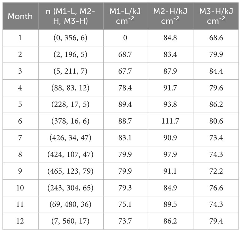
Table 2 The number and average TCHP of three typical water bodies with TCHP ≥ 60 kJ cm-2.
4.2 Distribution of different waters
The temporospatial distribution of these waters is shown in Figure 6. The data are categorized into north and south categories. The north and south are separated at 20°N. M1-H water mainly occurs in the northern NWP, and the number reaches a maximum in winter and a minimum in the TC season. Compared to the north of the NWP, the south of the NWP is dominated by M2-H water in winter. M1-L water generally appears in the south of the NWP, and M3-H water occurs in the north, both of which prevail in the TC season. Notably, a considerable amount of M2-H water exists in the TC season.
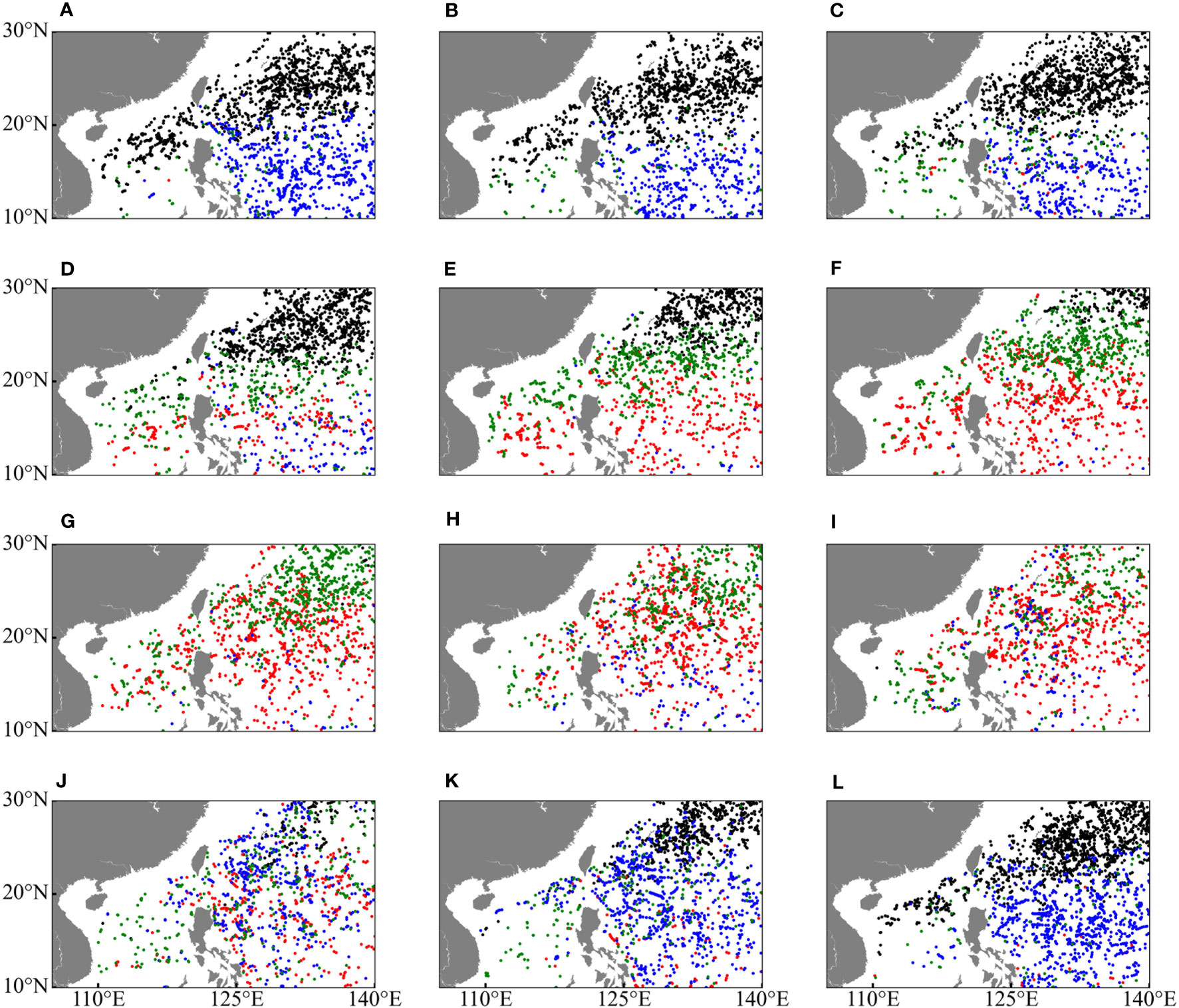
Figure 6 Spatial and temporal distribution of different water types. Black spots represent M1-H water, red spots represent M1-L water, blue spots represent M2-H water, and green spots represent M3-H water. (A–L) show the distribution of waters from January to December.
To further analyze the upper ocean structure, which is deeply influenced by upper ocean temperature and salinity, monthly mean temperature and salinity are averaged between 134.5°E and 135.5°E. In winter, the ILD is generally thick in the whole NWP. However, because of the latitude difference, the upper ocean at low latitudes is warmer than that at high latitudes (Figures 7A, K–L). Hence, the thermal conditions of the southern NWP are beneficial for TC development (Figure 1B). Moreover, due to the difference in local rainfall or meridional advection, sea surface salinity at high latitudes has a higher SSS than that at low latitudes. Convective precipitation is mainly distributed over the lower latitudes (Liu et al., 2012). Subsurface salinity at low latitudes is far higher than surface salinity (Figures 8A, K–L), and the difference between surface and subsurface salinity generates a thick barrier layer since the upper ocean at low latitudes is largely influenced by the North Equatorial Current (NEC), which usually carries high-salinity water (Schönau and Rudnick, 2015). The high solar radiation, plentiful precipitation, and NEC give the upper ocean at low latitudes characteristics of M2-H water. The small amount of precipitation and low solar radiation give the upper ocean at high latitudes characteristics of M1-H water. From spring to autumn, with increasing solar radiation, the SST in the whole NWP is maintained at a high level (Figures 7B–K), and a seasonal thermocline is generated in the whole NWP, greatly decreasing the mode 1 score and increasing the mode 3 score. Moreover, because the region with high precipitation moves to high latitudes (Liu et al., 2012), sea surface salinity decreases at high latitudes and thus generates a thick barrier layer (Figures 8B–K), which greatly increases the mode 3 score. Due to changes in solar radiation and precipitation, the upper ocean is characterized by M1-L water at low latitudes and M3-H water at high latitudes.
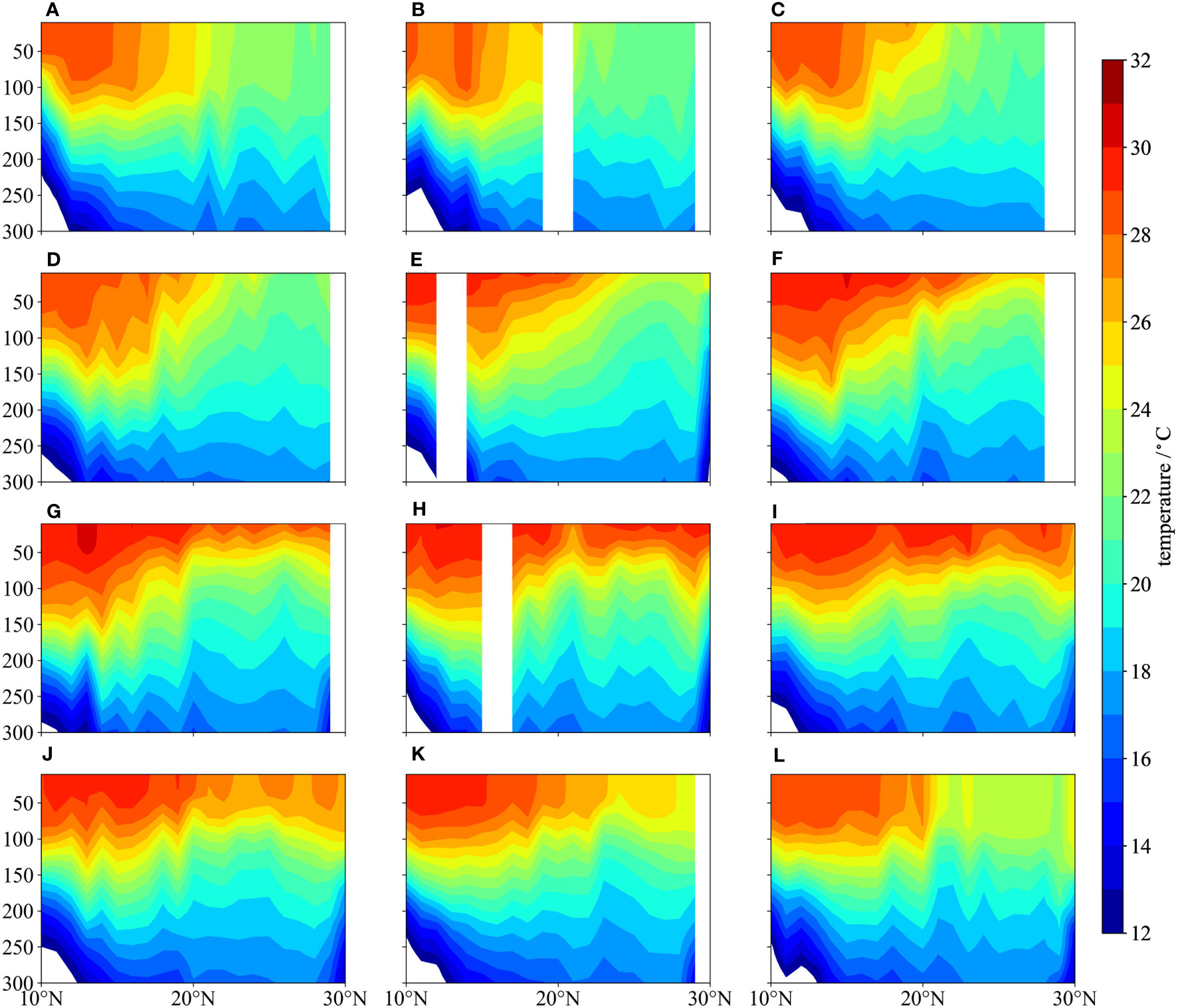
Figure 7 Latitude-depth sections of monthly mean temperature averaged between 134.5°E and 135.5°E. (A–L) show the mean temperature from January to December.

Figure 8 Latitude-depth sections of monthly mean salinity averaged between 134.5°E and 135.5°E. (A–L) show the mean salinity from January to December.
In addition to solar radiation, precipitation and NEC, mesoscale eddies also play a key role in the upper ocean structure (Pegliasco et al., 2022; Shay et al., 2000; Lin et al., 2008; Schiller and Ridgway, 2013). The isopycnal surfaces of anticyclonic eddies (AEs) with positive sea level anomalies (SLAs), known as warm-core eddies, exhibit a concave shape (Zhang et al., 2014). The upper isopycnal surface envelops a generous amount of warm water and outcrops at the sea surface. In contrast, cyclonic eddies (CEs) with negative SLAs, known as cold-core eddies, exhibit opposite structures compared with AEs. Profiles within AEs often also have the characteristics of M1-L water and M2-H water, while profiles within the CEs show characteristics of M3-H water. Since the number of eddies with a lifespan of 30 days (5451) is far more than that of eddies with lifespans of 90 (175) and 180 days (7), only eddies with a lifespan of 30 days are investigated here. Figure 9 depicts the locations of eddies encountered by TCs. The number of AEs (280) is smaller than that of CEs (321) within 300 kilometers of TCs, but the number of AEs (12) within 100 kilometers of TCs is visibly larger than that of CEs (4).
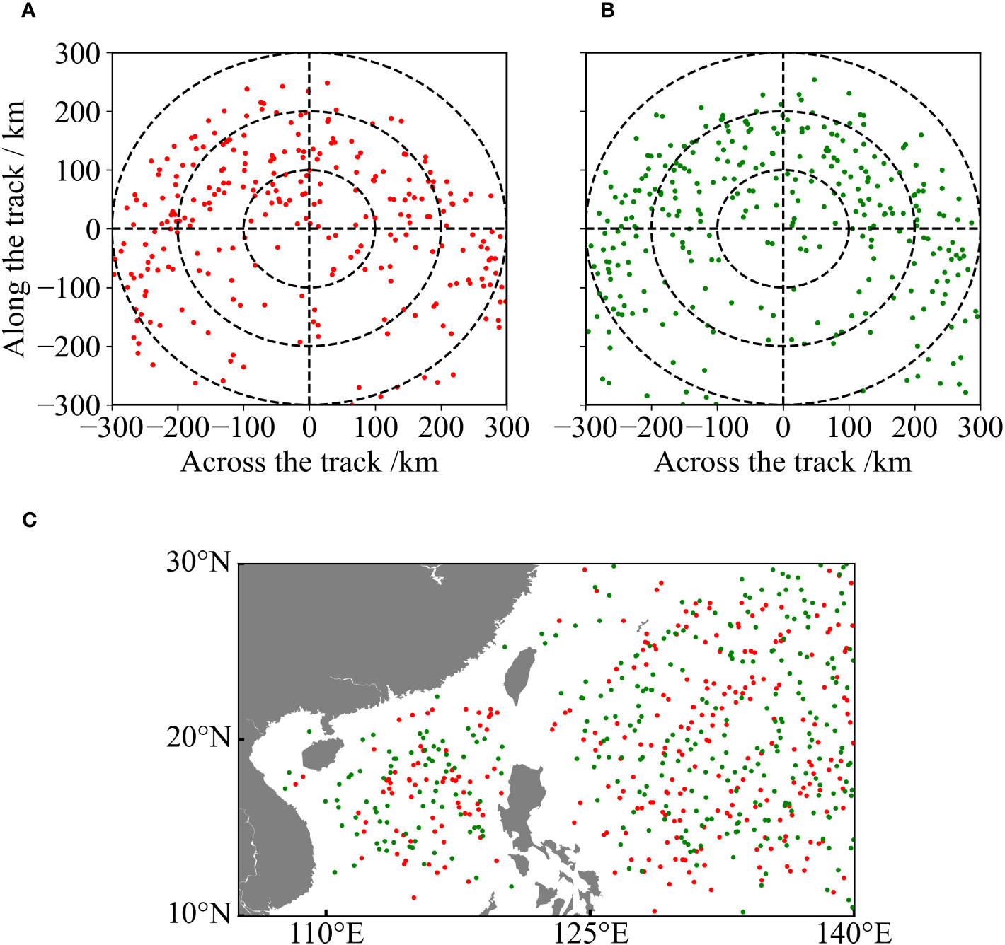
Figure 9 The distribution of AEs and CEs that TCs encountered between 2001 and 2020. (A) Distribution of AEs in the TCs. (B) Distribution of CEs in the TCs. (C) Distribution of AEs and CEs in the NWP. Red spots represent AEs, while green spots represent CEs.
4.3 Implications for TC development
TCs are mainly generated east of the Philippines and move toward the west or north because of the Pacific subtropical anticyclone. The difference in the proportion between the two directions is not obvious. However, the possibility of TC intensification is widely divergent. Figure 10A depicts the location when TCs begin to intensify during the TC season. Most TC intensification occurs in the southern NWP, and the proportion that occur in the north is quite small.
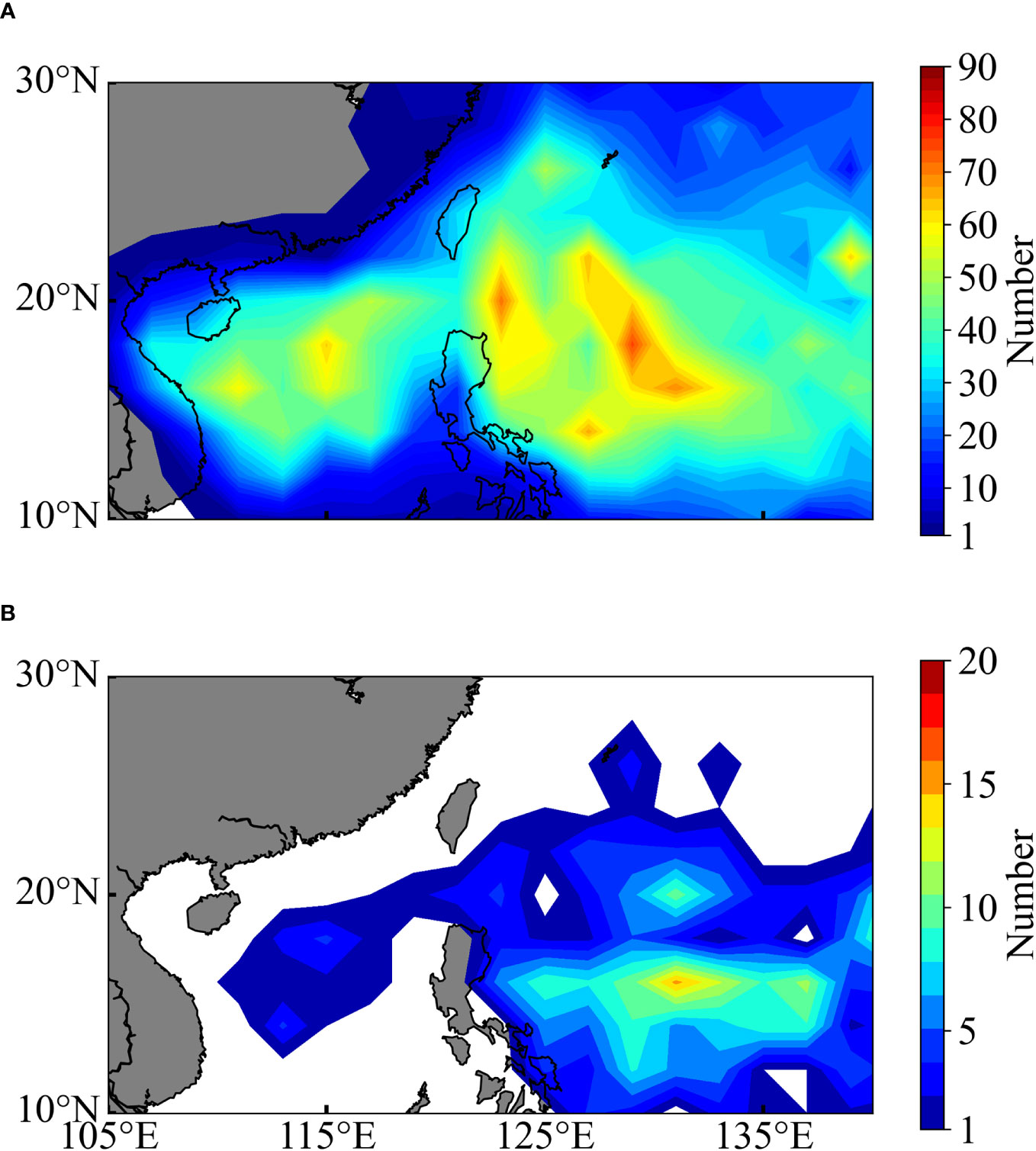
Figure 10 The location of TC intensification. (A) Distribution of TCs that began to intensify, (B) Distribution of rapid intensification.
Since this phenomenon is closely related to the upper ocean structure, the amount of each category of water that a TC encounters during the TC season is counted here and the temperature change during TC passage is further analyzed. To accurately calculate the temperature change during TC passage, two paired Argo profiles are identified through the following criteria: (1) the distance between the Argo profile and the TC center must be less than 300 km; (2) the distance between two paired profiles must be within 50 km, which can greatly reduce the differences in spatial variability in the ocean environment; (3) Argo profiles with a minimum observation depth shallower than 10 m and a maximum observation depth deeper than 300 m are extracted; and (4) the pre-TC profile observation time must be fewer than 5 days before TC passage, and the post-TC profile observation time must be within 3 days after TC passage. Following these conditions, 864 pairs of profiles are identified. With a one-dimensional mixed layer model, the temperature response of different waters to TCs is also investigated here. For each water type, all profiles with a maximum observation depth greater than 1000 m are identified. The averaged thermohaline profiles of different water types are created to initiate the 1DPWP model, as shown in Figure 11. For each simulated experiment, the 1DPWP model is run with 30-min time steps, and the averaged wind speed in TC categories between typhoons and super typhoons is applied.
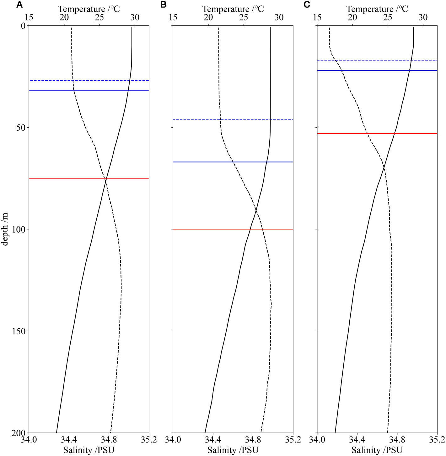
Figure 11 Averaged profiles of M1-L, M2-H and M3-H water. The black solid lines represent temperature and black dashed lines represent salinity. The blue solid lines indicate the ILD, blue dashed lines indicate the MLD, and red solid lines indicate the depths of the 26°C isotherm. (A) M1-L water. (B) M2-H water. (C) M3-H water.
The numbers of TCs that encounter M1-L water, M2-H water and M3-H water are 542, 306, and 216, respectively. M1-L and M2-H waters are mainly located in the south of the NWP. Notably, there are also considerable numbers of M1-L and M2-H water profiles in the northern Pacific, which is influenced by the Kuroshio. Moreover, the possibility of TC intensification is also large here. M3-H water mainly appears in the northern Pacific (Figures 6G–J). These results show that when a TC encounters M1-L water or M2-H water, it tends to intensify. The TCHPs of the M1-L, M2-H and M3-H water encountered by TCs are 68.9, 69.6 and 29.1 , respectively. The high TCHP of M1-L and M2-H causes TCs to rapidly intensify (Figure 10B), while M3-H water with low TCHP cannot provide sufficient heat energy for rapid intensification.
The mean and maximum SSTC induced by TCs is much lower for M2-H water relative to M1-L and M3-H water (Table 3). Moreover, although the SSTC of M1-L water is obvious, the SST of M1-L water is rather high and the modeled results show the same patterns (Figure 12). This reveals that the upper ocean structure obviously has a significant impact on the temperature response to strong TCs, which is important for TC intensification. Although the SST of M2-H water is the lowest, the BLD of M2-H water is the thickest, which reduces the SSTC by decreasing the entrainment rate caused by strong TCs. Thereby a TC intends to intensify rapidly, when it passes through upper ocean with M2-H characteristic. This result is also supported by Rudzin et al. (2017); Potter et al. (2019) and Rudzin et al. (2020). Moreover, the warm of M2-H water (Table 3) is also beneficial for low SSTC. Unlike that of M2-H water, the high SSTC of M1-L water is offset by its highest SST and warmest (Table 3). Therefore, the considerably high SST of M1-L water is still maintained, which is beneficial for TCs intensification. As the of M3-H water is cool (Table 3), and strong TCs can easily bring cold water to the surface, thus, high SST and thick BLD conditions play a small part in the sea surface cooling induced by strong TCs. Hence, it is hard for a TC to intensify when it meets M3-H water.
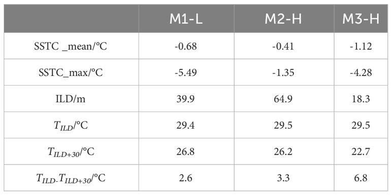
Table 3 SSTC, ILD, TILD and TILD+30 of three typical water tpyes caused by typhoons.
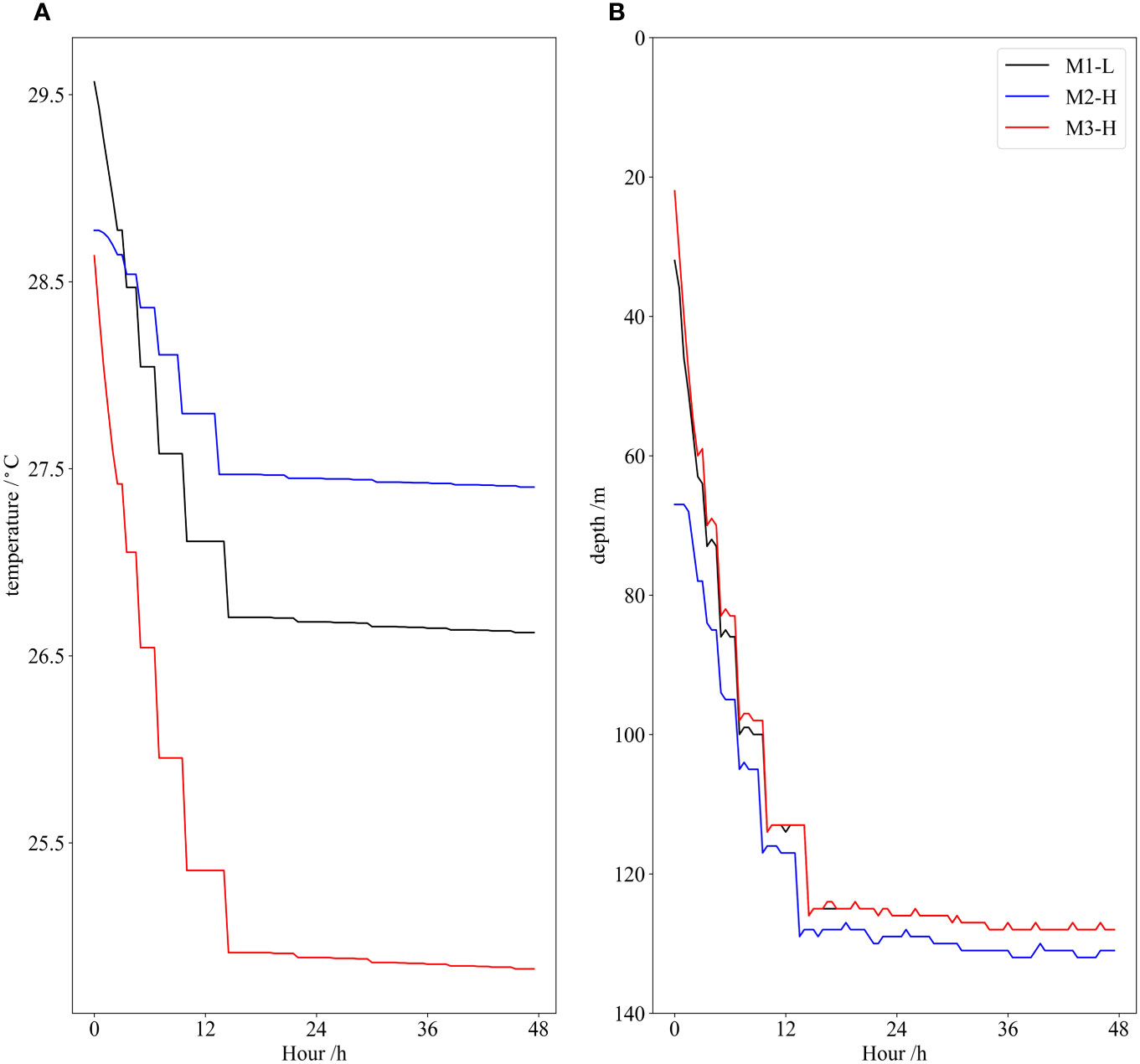
Figure 12 SST and ILD changes in different waters over 48 h of simulations. (A) SST changes. (B) ILD changes.
5 Summary and discussion
Many Argo profiles between 2001 and 2022 were used to investigate the upper ocean structure of the NWP. The SST, MLD, ILD, BLT, and OHC of each profile, which synthetically describe the thermal conditions and vertical stratification of the upper ocean structure, were calculated here. Moreover, to classify the upper ocean structure, these metrics were used in a principal component analysis. This study also adopted the 1DPWP model to explore the temperature response of each structure to TCs. The important findings are described as follows:
1) There are four different waters in the NWP. Profiles with low mode 1 scores (M1-L water) have an extremely warm and shallow layer with a narrow barrier layer covering the upper ocean, but profiles with high mode 1 scores (M1-H water) have a cold and thick layer in the upper ocean. A high mode 2 score (M2-H water) often means that profiles have a wide isothermal and mixed layer with a thick barrier layer. Both M1-L and M2-H water have a deep 26°C isotherm. Profiles with high mode 3 scores (M3-H water) have a shallow mixed layer with a comparatively deep barrier layer, 26°C isotherm, and relatively warm SST. Profiles for M1-L, M2-H and M3-H water have enough ocean heat content to support the development of TCs.
2) Different waters have different seasonal variations. M1-H water is located at high latitudes, and M2-H water is located at low latitudes during spring and winter. Low and high latitudes are separated at 20°N. With increasing solar radiation, M1-L and M3-H waters replace M2-H and M1-H waters. However, profiles at higher latitudes will also have characteristics of M1-L water and M2-H water between July and October. Moreover, M3-H water also appears at lower latitudes. This phenomenon is closely related to mesoscale eddies, with CEs making the vertical structure at lower latitudes exhibit M3-H water characteristics and AEs making the vertical structure at higher latitudes exhibit M1-L and M2-H water characteristics.
3) The relationship between TC intensification and the upper ocean structure in this study is investigated using observations and the 1DPWP model. When TCs pass the region with M3-H water characteristics, the possibility of TC intensification is small due to its high SSTC and low TCHP conditions. Both M1-L and M2-H waters with high TCHP values have a significant impact on TC intensification. However, the physical mechanisms of the two kinds of water are greatly different. The high SST and TCHP are maintained during TC intensification because of the large and high SST before the TC passage. Compared with M1-L water, the reason why a warm SST can be maintained in this water is its thickest BLD, which can largely decrease the rate of entrainment.
Although great progress has been made in understanding the physical mechanism of the interaction between TCs and the upper ocean, quantitative research on the upper ocean structure, especially the dynamic factors that influence the upper ocean structure before TC passage, is still lacking. As the results show, upper ocean structure has a great influence on TC intensification. Hence, how climate change affects the upper ocean structure is an important issue. Global warming increases rainfall over the south of NWP, which decreases sea surface salinity during TC season in this region (Balaguru et al., 2016). This situation increases the number of M2-H water that TCs encounter through making barrier layer thicker. Therefore, the probability of TC intensification in the south of NWP is increasing because of high TCHP of M2-H water.
M3-H water which plays a small part in TC intensification is significant in the north of NWP, and thereby analyzing the change of the number of M3-H water is essential. The water beneath the isothermal layer of M3-H water is actually Subtropical Mode Water (STMW) which is formed as deep-winter mixed layers south of the Kuroshio (Masuzawa, 1969). Isothermal layer tends to be shallower where STMW is thick (Oka et al., 2023) during TC season because STMW uplifts the overlying isotherms through the baroclinic adjustment mechanism (Xie et al., 2011). Hence, the number of M3-H water is greatly affected by the Kuroshio path variations south of Japan. The Kuroshio large mender reappeared and has persisted until now (Nishikawa et al., 2023; Qiu et al., 2023). Because of this reason, the westward advection of the colder variety of STMW from the region south of the Kuroshio Extension to the region north of NWP has been hindered, and therefore the thickness of STMW decrease notably in the north of NWP (Xu et al., 2017). In other word, the probability that the isothermal layer of upper ocean in the north of NWP deepen is increasing. On the other hand, the SST in the north of NWP has also increased rapidly due to global warming, which decreases the formation rate of colder variety of STMW south of Japan in winter (Hayashi et al., 2021; Hayashi et al., 2022). Observations in the recent years have proved this idea. As a result, the number of M3-H water presumably will decrease and the number of M1-L water and M2-H would be highly possible to appear in the north of NWP in the future. In other word, the probability of TC intensification will also generally increase in the north of NWP. Last, there is still progress to be made in upper ocean structure observing during TC season in the NWP in order to provide accurate upper ocean conditions in the case of global warming.
Additionally, it is insufficient to access SSTC through altimeter-derived TCHP or which means the average temperature from the sea surface to 100 m depth. For instance, even with a high TCHP, TC can still induce strong SSTC. Moreover, in the mid-latitude coastal regions, a shallow seasonal thermocline forms near the surface during summer, with cold water which is formed in winter below. Therefore, the entire ocean exhibits the similar characteristics of M3-H water. Despite the high TCHP or average temperature of the water column, weak TCs can still induce substantial surface cooling, thereby constraining the intensification of TCs. However, since the water column is well mixed, SSTC can be limited and the largest SSTC can also happen before TC passage, which are demonstrated in the research of Guan et al. (2021) and Glenn et al. (2016). Hence, it is necessary to establish continual and complete vertical structure observations in the shallow water and provide the accurate initial upper ocean conditions in coupled models.
Data availability statement
The raw data supporting the conclusions of this article will be made available by the authors, without undue reservation.
Author contributions
HZ and JY contributed to conception and design of the study. JY organized the database and performed the statistical analysis. JY wrote the first draft of the manuscript. HZ, HW, DT and JL wrote sections of the manuscript. All authors contributed to the article and approved the submitted version.
Funding
The author(s) declare financial support was received for the research, authorship, and/or publication of this article. This work was funded by the Project supported by the National Natural Science Foundation of China (42227901, 42176015), the Scientific Research Fund of the Second Institute of Oceanography, MNR (JG2309), the Innovation Group Project of Southern Marine Science and Engineering Guangdong Laboratory (Zhuhai) (311022001), the Project supported by Southern Marine Science and Engineering Guangdong Laboratory (Zhuhai) (SML2021SP207), the Shanghai Typhoon Research Foundation (TFJJ202111), and the key R&D Project of Zheijeng Province of China (2021C03186).
Conflict of interest
The authors declare that the research was conducted in the absence of any commercial or financial relationships that could be construed as a potential conflict of interest.
Publisher’s note
All claims expressed in this article are solely those of the authors and do not necessarily represent those of their affiliated organizations, or those of the publisher, the editors and the reviewers. Any product that may be evaluated in this article, or claim that may be made by its manufacturer, is not guaranteed or endorsed by the publisher.
Supplementary material
The Supplementary Material for this article can be found online at: https://www.frontiersin.org/articles/10.3389/fmars.2023.1245348/full#supplementary-material
References
Balaguru K., Chang P., Saravanan R., Leung L. R., Xu Z., Li M., et al. (2012). Ocean barrier layers’ effect on tropical cyclone intensification. Proc. Natl. Acad. Sci. U.S.A. 109, 14343–14347. doi: 10.1073/pnas.1201364109
Balaguru K., Foltz G. R., Leung L. R., Emanuel K. A. (2016). Global warming-induced upper-ocean freshening and the intensification of super typhoons. Nat. Commun. 7, 13670. doi: 10.1038/ncomms13670
Chan J. C. L., Duan Y. (2001). Tropical cyclone intensity change from a simple ocean-atmosphere coupled model. J. Atmospheric Sci. 58, 154–172. doi: 10.1175/1520-0469(2001)058<0154:tcicfa>2.0.co;2
De Boyer Montégut C., Mignot J., Lazar A., Cravatte S. (2007). Control of salinity on the mixed layer depth in the world ocean: 1. General description. J. Geophysical Res. 112. doi: 10.1029/2006jc003953
DeMaria M., Sampson C. R., Knaff J. A., Musgrave K. D. (2014). Is tropical cyclone intensity guidance improving? Bull. Am. Meteorological Soc. 95, 387–398. doi: 10.1175/bams-d-12-00240.1
Emanuel K. (2005). Increasing destructiveness of tropical cyclones over the past 30 years. Nature 436, 686–688. doi: 10.1038/nature03906
Glenn S. M., Miles T. N., Seroka G. N., Xu Y., Forney R. K., Yu F., et al. (2016). Stratified coastal ocean interactions with tropical cyclones. Nat. Commun. 7 (1), 10887. doi: 10.1038/ncomms10887
Guan S., Zhao W., Sun L., Zhou C., Liu Z., Hong X., et al. (2021). Tropical cyclone-induced sea surface cooling over the Yellow Sea and Bohai Sea in the 2019 Pacific typhoon season. J. Mar. Syst. 217, 103509. doi: 10.1016/j.jmarsys.2021.103509
Hayashi M., Shiogama H., Emori S., Ogura T., Hirota N. (2021). The northwestern Pacific warming record in August 2020 occurred under anthropogenic forcing. Geophysical Res. Lett. 48 (1), e2020GL090956. doi: 10.1029/2020GL090956
Hayashi M., Shiogama H., Ogura T. (2022). The contribution of climate change to increasing extreme ocean warming around Japan. Geophysical Res. Lett. 49 (19), e2022GL100785. doi: 10.1029/2022GL100785
He S., Cheng X., Fei J., Wei Z., Huang X., Liu L. (2022). Thermal response to tropical cyclones over the Kuroshio. Earth Space Sci. 9. doi: 10.1029/2021ea002001
Holliday C. R., Thompson A. H. (1979). Climatological characteristics of rapidly intensifying typhoons. Monthly Weather Rev. 107, 1022–1034. doi: 10.1175/1520-0493(1979)107<1022:ccorit>2.0.co;2
Kawakami Y., Nakano H., Urakawa L. S., Toyoda T., Sakamoto K., Yoshimura H., et al. (2022). Interactions between ocean and successive typhoons in the kuroshio region in 2018 in atmosphere–ocean coupled model simulations. J. Geophysical Research: Oceans 127. doi: 10.1029/2021jc018203
Kossin J. P., DeMaria M. (2016). Reducing operational hurricane intensity forecast errors during eyewall replacement cycles. Weather Forecasting 31, 601–608. doi: 10.1175/waf-d-15-0123.1
Leipper D. F., Volgenau L. D. (1972). Hurricane heat potential of the gulf of Mexico. J. Phys. Oceanpgr. 2, 218–224. doi: 10.1175/1520-0485(1972)002<0218:hhpotg>2.0.co;2
Li J., Sun L., Yang Y., Cheng H. (2020). Accurate evaluation of sea surface temperature cooling induced by typhoons based on satellite remote sensing observations. Water 12(5), 1413. doi: 10.3390/w12051413
Lin I.-I., Wu C.-C., Pun I.-F., Ko D.-S. (2008). Upper ocean thermal structure and the Western North Pacific category-5 typhoons part I: ocean features and category-5 typhoon’s intensification. Monthly Weather Rev. 136, 3288–3306. doi: 10.1175/2008MWR2277.1
Lin S., Zhang W.-Z., Shang S.-P., Hong H.-S. (2017). Ocean response to typhoons in the western North Pacific: Composite results from Argo data. Deep Sea Res. Part I: Oceanographic Res. Papers 123, 62–74. doi: 10.1016/j.dsr.2017.03.007
Liu T., Abernathey R. (2023). A global Lagrangian eddy dataset based on satellite altimetry. Earth System Sci. Data 15, 1765–1778. doi: 10.5194/essd-15-1765-2023
Liu Z., Li Z., Lu S., Wu X., Sun C., Xu J. (2021). Scattered data set of temperature and salinity profiles from the international Argo program over the global ocean. Global Change Res. Data Publishing Repository. doi: 10.3974/geodb.2021.06.05.V1
Liu P., Li C., Wang Y., Fu Y. (2012). Climatic characteristics of convective and stratiform precipitation over the Tropical and Subtropical areas as derived from TRMM PR. Sci. China Earth Sci. 56, 375–385. doi: 10.1007/s11430-012-4474-4
Lyu X., Wang X., Leslie L. M. (2019). The dependence of Northwest Pacific tropical cyclone intensification rates on environmental factors. Adv. Meteorol. 2019, 1–18. doi: 10.1155/2019/9456873
Mainelli M., Demaria M., Shay L. K., Goni G. (2008). Application of oceanic heat content estimation to operational forecasting of recent Atlantic category 5 hurricanes. Weather Forecasting 23, 3–16. doi: 10.1175/2007WAF2006111.1
Masuzawa J. (1969). Subtropical mode water. Deep sea Res. oceanographic abstracts 16(5), 463–472. doi: 10.1016/0011-7471(69)90034-5
Nishikawa H., Oka E., Sugimoto S. (2023). Subtropical Mode Water in a recent persisting Kuroshio large-meander period: Part II—formation and temporal evolution in the Kuroshio recirculation gyre off Shikoku. J. Oceanogr. 79, 461–471. doi: 10.1007/s10872-023-00689-2
Oka E., Sugimoto S., Kobashi F., Nishikawa H., Kanada S., Nasuno T., et al. (2023). Subtropical Mode Water south of Japan impacts typhoon intensity. Sci. Adv. 9 (37), eadi2793. doi: 10.1126/sciadv.adi2793
Park J. J., Kwon Y.-O., Price J. F. (2011). Argo array observation of ocean heat content changes induced by tropical cyclones in the north Pacific. J. Geophysical Res. 116. doi: 10.1029/2011jc007165
Pegliasco C., Delepoulle A., Mason E., Morrow R., Faugère Y., Dibarboure G. (2022). META3.1exp: a new global mesoscale eddy trajectory atlas derived from altimetry. Earth System Sci. Data 14, 1087–1107. doi: 10.5194/essd-14-1087-2022
Potter H., DiMarco S. F., Knap A. H. (2019). Tropical cyclone heat potential and the rapid intensification of hurricane harvey in the Texas bight. J. Geophysical Research: Oceans 124 (4), 2440–2451. doi: 10.1029/2018JC014776
Potter H., Rudzin J. E. (2021). Upper-ocean temperature variability in the gulf of Mexico with implications for hurricane intensity. J. Phys. Oceanogr. 51, 3149–3162. doi: 10.1175/jpo-d-21-0057.1
Powell M. D., Vickery P. J., Reinhold T. A. (2003). Reduced drag coefficient for high wind speeds in tropical cyclones. Nature 422, 279–283. doi: 10.1038/nature01481
Price J. F. (1981). Upper ocean response to a hurricane. J. Phys. Oceanogr. 11, 153–175. doi: 10.1175/1520-0485(1981)011<0153:UORTAH>2.0.CO;2
Price J. F., Weller R. A., Pinkel R. (1986). Diurnal cycling: Observations and models of the upper ocean response to diurnal heating, cooling, and wind mixing. J. Geophysical Res. 91, 8411–8427. doi: 10.1029/JC091iC07p08411
Qiu B., Chen S., Oka E. (2023). Why did the 2017 Kuroshio large meander event become the longest in the past 70 years? Geophysical Res. Lett. 50 (10), e2023GL103548. doi: 10.1029/2023GL103548
Rudzin J. E., Chen S., Sanabia E. R., Jayne S. R. (2020). The air-sea response during hurricane Irma’s, (2017) rapid intensification over the amazon-orinoco river plume as measured by atmospheric and oceanic observations. J. Geophysical Research: Atmospheres 125 (18), e2019JD032368. doi: 10.1029/2019JD032368
Rudzin J. E., Shay L. K., Jaimes B., Brewster J. K. (2017). Upper ocean observations in eastern Caribbean Sea reveal barrier layer within a warm core eddy. J. Geophysical Research: Oceans 122 (2), 1057–1071. doi: 10.1002/2016jc012339
Schiller A., Ridgway K. R. (2013). Seasonal mixed-layer dynamics in an eddy-resolving ocean circulation model. J. Geophysical Research: Oceans 118, 3387–3405. doi: 10.1002/jgrc.20250
Schönau M. C., Rudnick D. L. (2015). Glider observations of the North Equatorial Current in the western tropical Pacific. J. Geophysical Research: Oceans 120, 3586–3605. doi: 10.1002/2014jc010595
Shay L. K., Goni G. J., Black P. G. (2000). Effects of a warm oceanic feature on hurricane opal. Monthly Weather Rev. 128, 1366–1383. doi: 10.1175/1520-0493(2000)128<1366:EOAWOF>2.0.CO;2
Shay L. K., Jaimes B., Uhlhorn E. W. (2015). Enthalpy and momentum fluxes during hurricane earl relative to underlying ocean features. Monthly Weather Rev. 143, 111–131. doi: 10.1175/mwr-d-13-00277.1
Tao D., Zhang F. (2014). Effect of environmental shear, sea-surface temperature, and ambient moisture on the formation and predictability of tropical cyclones: An ensemble-mean perspective. J. Adv. Modeling Earth Syst. 6, 384–404. doi: 10.1002/2014ms000314
Vincent E. M., Lengaigne M., Vialard J., Madec G., Jourdain N. C., Masson S. (2012). Assessing the oceanic control on the amplitude of sea surface cooling induced by tropical cyclones. J. Geophysical Research: Oceans 117, n/a–n/a. doi: 10.1029/2011jc007705
Wada A., Chan J. C. L. (2008). Relationship between typhoon activity and upper ocean heat content. Geophysical Res. Lett. 35. doi: 10.1029/2008gl035129
Wada A., Usui N., Sato K. (2012). Relationship of maximum tropical cyclone intensity to sea surface temperature and tropical cyclone heat potential in the North Pacific Ocean. J. Geophysical Research: Atmospheres 117. doi: 10.1029/2012jd017583
Wang X., Han G., Qi Y., Li W. (2011). Impact of barrier layer on typhoon-induced sea surface cooling. Dynamics Atmospheres Oceans 52, 367–385. doi: 10.1016/j.dynatmoce.2011.05.002
Wang Y.-Q., Wu C.-C. (2004). Current understanding of tropical cyclone structure and intensity changes–a review. Meteorol. Atmospheric Phys. 87, 257–278. doi: 10.1007/s00703-003-0055-6
Wang G., Wu L., Johnson N. C., Ling Z. (2016). Observed three-dimensional structure of ocean cooling induced by Pacific tropical cyclones. Geophysical Res. Lett. 43, 7632–7638. doi: 10.1002/2016gl069605
Wu C.-R., Chang Y.-L., Oey L.-Y., Chang C. W. J., Hsin Y.-C. (2008). Air-sea interaction between tropical cyclone Nari and Kuroshio. Geophysical Res. Lett. 35, n/a–n/a. doi: 10.1029/2008gl033942
Xie S.-P., Xu L., Liu Q., Kobashi F. (2011). Dynamical role of mode water ventilation in decadal variability in the central subtropical gyre of the North Pacific. J. Climate 24 (4), 1212–1225. doi: 10.1175/2010JCLI3896.1
Xu L., Xie S. P., Liu Q., Liu C., Li P., Lin X. (2017). Evolution of the North Pacific subtropical mode water in anticyclonic eddies. J. Geophysical Research: Oceans 122 (12), 10118–10130. doi: 10.1002/2017JC013450
Yan Y., Li L., Wang C. (2017). The effects of oceanic barrier layer on the upper ocean response to tropical cyclones. J. Geophysical Research: Oceans 122, 4829–4844. doi: 10.1002/2017jc012694
Zhang H., Chen D., Zhou L., Liu X., Ding T., Zhou B. (2016). Upper ocean response to typhoon Kalmaegi, (2014). J. Geophysical Research: Oceans 121, 6520–6535. doi: 10.1002/2016jc012064
Zhang H., He H., Zhang W.-Z., Tian D. (2021). Upper ocean response to tropical cyclones: a review. Geosci. Lett. 8. doi: 10.1186/s40562-020-00170-8
Zhang Z., Wang W., Qiu B. (2014). Oceanic mass transport by mesoscale eddies. Science 345, 322–324. doi: 10.1126/science.1252418
Keywords: vertical structure, thermal conditions, Northwest Pacific Ocean, sea surface cooling, tropical cyclones
Citation: Yu J, Zhang H, Wang H, Tian D and Li J (2023) Upper-ocean structure variability in the Northwest Pacific Ocean in response to tropical cyclones. Front. Mar. Sci. 10:1245348. doi: 10.3389/fmars.2023.1245348
Received: 23 June 2023; Accepted: 07 November 2023;
Published: 24 November 2023.
Edited by:
Matthieu Le Hénaff, University of Miami, United StatesReviewed by:
Karthik Balaguru, Pacific Northwest National Laboratory (DOE), United StatesShoude Guan, Ocean University of China, China
Copyright © 2023 Yu, Zhang, Wang, Tian and Li. This is an open-access article distributed under the terms of the Creative Commons Attribution License (CC BY). The use, distribution or reproduction in other forums is permitted, provided the original author(s) and the copyright owner(s) are credited and that the original publication in this journal is cited, in accordance with accepted academic practice. No use, distribution or reproduction is permitted which does not comply with these terms.
*Correspondence: Han Zhang, emhhbmdoYW5Ac2lvLm9yZy5jbg==; Huizan Wang, d2FuZ2h1aXphbjE3QG51ZHQuZWR1LmNu