Long-term trends and extreme events of marine heatwaves in the Eastern China Marginal Seas during summer

Marine heatwaves (MHWs) are a type of widespread, persistent, and extreme marine warming event that can cause serious harm to the global marine ecology and economy. This study provides a systematic analysis of the long-term trends of MHWs in the Eastern China Marginal Seas (ECMS) during summer spanning from 1982 to 2022, and occurrence mechanisms of extreme MHW events. The findings show that in the context of global warming, the frequency of summer MHWs in the ECMS has increased across most regions, with a higher rate along the coast of China. Areas exhibiting a rapid surge in duration predominantly reside in the southern Yellow Sea (SYS) and southern East China Sea (ECS, south of 28°N). In contrast, the long-term trends of mean and maximum intensities exhibit both increases and decreases: Rising trends primarily occur in the Bohai Sea (BS) and Yellow Sea (YS), whereas descending trends are detected in the northern ECS (north of 28°N). Influenced jointly by duration and mean intensity, cumulative intensity (CumInt) exhibits a notable positive growth off the Yangtze River Estuary, in the SYS and southern ECS. By employing the empirical orthogonal function, the spatio-temporal features of the first two modes of CumInt and their correlation with summer mean sea surface temperature (SST) and SST variance are further examined. The first mode of CumInt displays a positive anomalous pattern throughout the ECMS, with notable upward trend in the corresponding time series, and the rising trend is primarily influenced by summer mean SST warming. Moreover, both of the first two modes show notable interannual variability. Extreme MHW events in the SYS in 2016 and 2018 are examined using the mixed layer temperature equation. The results suggest that these extreme MHW events originate primarily from anomalous atmospheric forcing and oceanic vertical mixing. These processes involve an anomalous high-pressure system over the SYS splitting from the western Pacific subtropical high, augmented atmospheric stability, diminished wind speeds, intensified solar radiation, and reduced oceanic mixing, thereby leading to the accumulation of more heat near the sea surface and forming extreme MHW events.

1 Introduction

Marine heatwaves (MHWs) are defined as anomalous warming events where sea surface temperature (SST) exceeds a specific threshold during certain periods (Hobday et al., 2016; Frölicher et al., 2018). With the ongoing rise of global SST, the strength of MHW events has significantly increased (Frölicher et al., 2018; Oliver et al., 2018; Smale et al., 2019). A 1°C increase in SST corresponds to an increase of 3.7 events in frequency, an additional 7.5 days in duration, and a 2.2°C rise in maximum intensity (Cheng et al., 2023). Projections indicate that in the future, MHWs will continue to evolve towards more frequent, longer-lasting, and more extreme events (Hayashida et al., 2020; Laufkötter et al., 2020; Holbrook et al., 2021; Qiu et al., 2021; Yao et al., 2022b). Extreme MHW events can lead to localized heat stress accumulation, potentially exceeding ecosystem thresholds and causing irreversible damage to marine ecosystems (Frölicher et al., 2018; Genevier et al., 2019; Garrabou et al., 2022). This includes loss of marine biological habitats, large-scale species migration or mortality (Garrabou et al., 2009; Feng et al., 2013; Mills et al., 2013; Caputi et al., 2016; Frölicher and Laufkötter, 2018; Cheung and Frölicher, 2020), and poses significant risks to marine economies and human living environment (Hughes et al., 2017; Oliver et al., 2017, Oliver et al., 2019; Holbrook et al., 2020; Jacox et al., 2022; Pastor and Khodayar, 2023).

The Eastern China Marginal Seas [ECMS, including the Bohai Sea (BS), Yellow Sea (YS), and East China Sea (ECS)], depicted in Figure 1A, is recognized as one of the largest continental shelf seas globally, boasts a rich diversity of species and notable productivity. Additionally, it serves as a primary hotspot area for global MHW events (Belkin, 2009; Lima and Wethey, 2012; Bao and Ren, 2014; Hobday and Pecl, 2014; Oliver et al., 2018, Oliver et al., 2021; Xu et al., 2022). In the past 40 years, MHW events in the ECMS have significantly increased, and the growth rates have escalated to more than double the global mean growth rates (Li et al., 2019; Yao et al., 2020; Lee et al., 2023). For instance, the mean MHW intensity in the ECMS has increased by 0.1 to 0.3°C/decade, higher than the global average growth rate of 0.085°C/decade (Yao et al., 2020). Oliver (2019) suggested that changes in both mean SST and SST variance can affect MHW trends. Lee et al. (2023) found robust positive trends in the summer MHW frequency, total days, and maximum intensity off the Yangtze River Estuary, and pointed out that the summer MHW trend is primarily due to rapidly increasing mean SST.

Figure 1

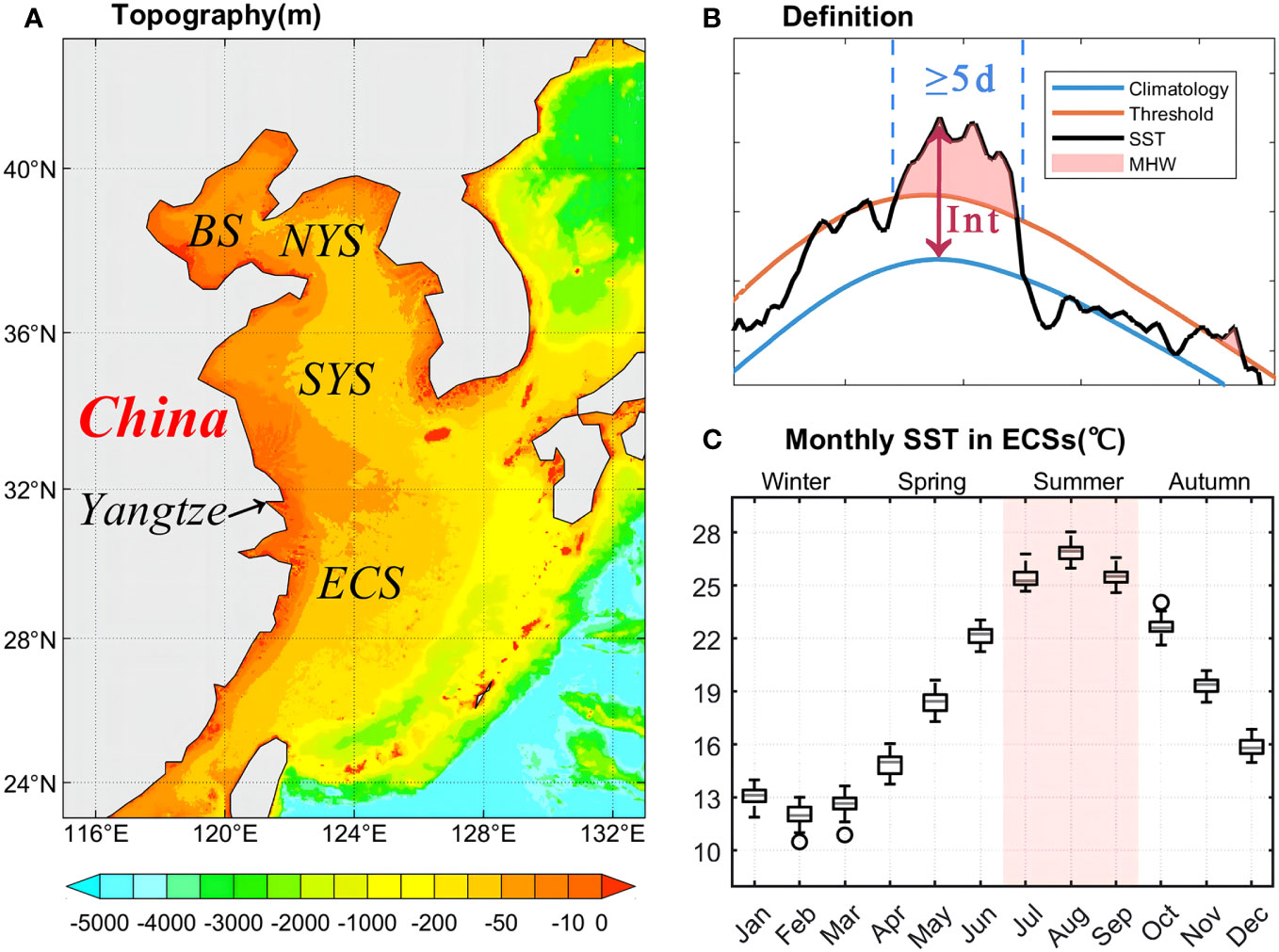
Figure 1 (A) Map of the Eastern China Marginal Seas (ECMS) with topography. The ECMS include the Bohai Sea (BS), northern Yellow Sea (NYS), southern Yellow Sea (SYS), and East China Sea (ECS). (B) Schematic diagram of the definition of MHWs. (C) Boxplot of monthly SST climatology in the ECMS.

In recent years, heightened focus has emerged on exploring the physical dynamics behind the frequent occurrence of extreme MHW events in the ECMS during summer (Gao et al., 2020; Lee et al., 2020; Yan et al., 2020; Li et al., 2022, Li et al., 2023; Tan et al., 2023; Oh et al., 2023a). Studies indicate that extreme events in the ECMS are largely driven by anomalous atmospheric conditions and oceanic processes. For example, Yan et al. (2020) found that in summer 2016, the SST in the southern YS (SYS) and northern ECS peaked at 29.68°C, a record-breaking value. This unprecedented temperature was attributed to the synergistic effects of enhanced solar radiation and reduced wind speed under anomalous subtropical high-pressure system. Gao et al. (2020) reported a pattern of intense MHW events over three consecutive summers from 2016 to 2018. These events were primarily correlated with anomalous changes in shortwave radiation, advection, and vertical mixing. Li et al. (2023) observed a peak MHW intensity of 5.15°C in the northern YS (NYS) in the summer of 2018. They suggested that the intensification of incidents is a consequence of a robust subsidence motion that ensued from the northward migration of the western Pacific subtropical high and the northeastward enlargement of the South Asian high. Further, Tan et al. (2023) and Oh et al. (2023a) revealed a record-setting event in the SYS and ECS during the summer of 2022 that spanned 62 days, a duration six times longer than average. This elongated occurrence was instigated by a surge in the outflow from the Yangtze-Huai River floods. Concurrently, a persistent anticyclonic circulation increased solar radiation, contributing to an extended duration of the MHW (Oh et al., 2023a).

As forementioned, many studies have been held on the role of changes in mean SST and SST variance in influencing MHW long-term trends (Oliver et al., 2018; Holbrook et al., 2019; Jacox, 2019; Oliver, 2019; Qi et al., 2022; Wang et al., 2022; Yao and Wang, 2022; Yao et al., 2022a; Cheng et al., 2023). However, studies concerning the ECMS remain limited, and no effective research to date has elucidated the spatio-temporal evolution of summer MHWs in response to the warming SST. To bridge this knowledge gap, we employed observational and reanalysis datasets to analyze spatio-temporal changes in MHWs amid the warming trend, particularly focusing on the impacts of changes in mean SST and SST variance on the long-term trends of summer MHWs. In addition, as for the dynamic mechanisms, the respective contributions of atmospheric and oceanic processes remain controversial. We conducted a quantitative analysis of the dynamics underlying extreme events, utilizing the mixed layer temperature (MLT) equation, to enhance our understanding of their generation processes.

This paper is structured as follows: Section 2 introduces the data, defines MHWs, and outlines the research methods utilized. Section 3 presents the long-term trends of MHWs in the ECMS during summer, with a focus on the two primary modes of MHWs, and also investigates the role of changes in mean SST and SST variance. Subsequently, following a classification of MHW events, we delve into the dynamic mechanisms of extreme events. Section 4 summarizes the results.

2 Data and methods

2.1 Data

This study employs the daily Optimum Interpolation Sea Surface Temperature v2 (OISST v2) dataset from the National Oceanic and Atmospheric Administration (NOAA) to detect MHWs (Reynolds et al., 2007; Huang et al., 2021). The OISST dataset amalgamates observations from diverse sources, such as ocean satellites, ships, buoys, and Argo floats. Spanning continuously from September 1, 1981, to the present, the dataset offers a spatial resolution of 0.25° × 0.25°. Access and download of the data are available at the following link: https://downloads.psl.noaa.gov/.

To examine the dynamic mechanisms underlying MHWs, temperature and salinity profiles, along with horizontal and vertical ocean current velocities and net surface heat flux, from the Ocean general circulation model For the Earth Simulator (OFES) dataset (Sasaki et al., 2008) are utilized. This ocean circulation model, developed in Japan, has a vertical resolution of 5 m at the surface, with a spatial resolution of 0.1° × 0.1° and a temporal resolution of three days. The data is available for download at http://apdrc.soest.hawaii.edu/. Yan et al. (2020) have validated the vertical structure of temperature and salinity simulated by OFES and confirmed that OFES is capable of reproducing the dynamics of the mixed layer (ML) in the ECMS.

Supplementing the analysis of physical processes responsible for MHW generation, atmospheric data such as geopotential height, wind fields, surface shortwave radiation, and total cloud cover are also incorporated from the Fifth Generation of the European Centre for Medium-Range Weather Forecasts (ECMWF) reanalysis data, also known as ERA5 (Hersbach et al., 2020). This dataset, with a spatial resolution of 0.25° × 0.25° and a temporal resolution of one hour, is available for download at https://cds.climate.copernicus.eu/.

2.2 MHW identification

In this study, the identification of MHWs adheres to the seasonal threshold method proposed by Hobday et al. (2016), utilizing the daily OISST spanning 1982-2022. Specifically, a MHW event is defined at each grid point when the daily SST surpasses the threshold (T₉₀, the 90^th percentile of the daily SST over a 41-year historical baseline period) for five consecutive days or more (Figure 1B). If the interval between two events is two days or less, it is regarded as a single continuous MHW event. The 90^th percentile threshold is computed by taking the daily SST values within an 11-day window centered on each day, determining the corresponding 90^th percentile threshold for that date, and subsequently smoothing the threshold using a 31-day moving average (Oliver et al., 2019; Plecha and Soares, 2020). To mitigate statistical biases due to abnormal increase or decrease of stages, the entire research period is selected as the baseline period for climatological calculation. Key characteristics describing MHW events include frequency, duration, total days, intensity, and cumulative intensity (Oliver et al., 2018; Hayashida et al., 2020). Herein, “frequency” denotes the number of MHW events, “duration” signifies the time span from an event’s start to its end, “total days” refers to the cumulative number of heatwave days, “intensity” is the SST anomaly above the climatological mean during the MHW period, and “cumulative intensity” is the cumulative SST anomaly during an MHW event. These specific definitions are elaborated in Table 1. To investigate MHWs during summer, we have divided the data into four distinct seasons. The three months (July-August-September, JAS) with higher MHW occurrence frequency, broader range (Supplementary Figure S1) and the highest average SST (Figure 1C) were defined as summer.

Table 1

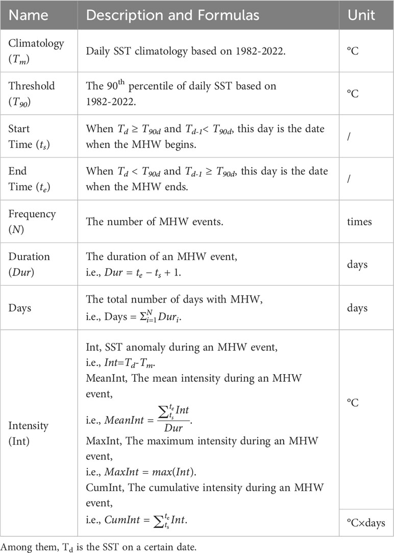
Table 1 Definitions of MHW properties.

2.3 MHW intensity classification

In this study, the categorization of MHW intensity integrates previous classification methods (Hobday et al., 2018; Oliver et al., 2019) and takes into account the characteristics of events in the ECMS. Event intensity is classified into three severity categories based on multiples of the 90^th percentile difference from the mean climatology value, as delineated in Equation (1): Moderate ($1\le L<1.5$), Strong ($1.5\le L<2$), and Extreme ($L\ge 2$ ). This approach enables a nuanced statistical analysis of the events. The brief formula is as follows.

$\begin{array}{ll}L=\frac{T_d-T_m}{T_{90}-T_m}& (1)\end{array}$

Herein, L denotes the event’s grading level, $T_d$ signifies the daily SST, $T_m$ indicates the climatology of temperature, and $T_{90}$ defines the threshold for event identification.

2.4 EOF analysis

To elucidate the primary spatio-temporal features of MHWs, Empirical Orthogonal Function (EOF) analysis is adopted in this study (Lorenz, 1956). This method decomposes the data pertaining to CumInt, mean intensity (MeanInt), and duration of MHWs into spatial patterns and corresponding time series as illustrated below (Equation 2):

$\begin{array}{ll}\mathit{\text{X}}(\mathit{\text{t}})={\sum }_{\mathit{\text{i}}=\mathbf{1}}^{\mathit{\text{N}}}\mathit{\text{P}}{\mathit{\text{C}}}_{\mathit{\text{i}}}(\mathit{\text{t}})\times \mathit{\text{EO}}{\mathit{\text{F}}}_{\mathit{\text{i}}}& (2)\end{array}$

where $X(t)$ represents the multi-dimensional data vector corresponding to the time t, $P{C}_i(t)$ is the principal component (PC) time series of the i-th mode, $EO{F}_i$ is the corresponding spatial pattern (EOF), N is the total number of modes. This decomposition allows us to identify and analyze the dominant spatial patterns in the data and their changes over time.

Through EOF analysis, we can simplify the complex spatio-temporal dataset into a set of spatial patterns and time series, greatly facilitates our understanding and explanation of the main patterns and trends in data changes. The significance of the EOF modes is assessed using the North statistical test (North et al., 1982). Notably, linear trends in MHWs are not removed during these computations to preserve their long-term trends.

2.5 MLT equation

To investigate the primary drivers of Extreme MHW events, we conducted a MLT equation analysis, which has been widely used in previous studies (Amaya et al., 2020; Yan et al., 2020; Lee et al., 2022a; Liu et al., 2022; Oh et al., 2023a). This approach facilitates the quantitative evaluation of various factors’ relative contributions to the MLT tendency term (Moisan and Niiler, 1998). The equation is as follows:

$\begin{array}{ll}\frac{\partial {\mathit{\text{T}}}_{\mathit{\text{mld}}}}{\mathbf{\text{∂t}}}=-({\overrightarrow{\mathit{\text{V}}}}_{\mathit{\text{mld}}}·\nabla {\mathit{\text{T}}}_{\mathit{\text{mld}}})-{\mathit{\text{w}}}_{\mathit{\text{ent}}}\frac{({\mathit{\text{T}}}_{\mathit{\text{mld}}}-{\mathit{\text{T}}}_{\mathit{\text{below}}})}{{\mathit{\text{h}}}_{\mathit{\text{mld}}}}+\frac{\mathit{\text{Hflx}}-{\mathit{\text{q}}}_{\mathit{\text{h}}}}{\mathit{\text{ρ}}{\mathit{\text{C}}}_{\mathit{\text{p}}}{\mathit{\text{h}}}_{\mathit{\text{mld}}}}& (3)\end{array}$

In the equation, $T_{mld}$ denotes the average water temperature within the ML and $T_{below}$ denotes water temperature below the ML. ${\overrightarrow{V}}_{mld}$ represents the average horizontal velocity within the ML and $w_{ent}$ represents the entrainment velocity across the bottom of the ML. $h_{mld}$ is the ML depth (MLD). $Hflx$ is the surface net heat flux and $q_h$ is the downward radiative heat flux at the bottom of the ML. ρ represents the reference density of seawater (1025 kg m^-3), and $C_P$ is the specific heat of seawater at constant pressure (4000 J kg^-1 K^-1). Following Qu (2001) and Yan et al. (2020), the entrainment velocity is calculated as (Equation 4):

$\begin{array}{ll}{\mathit{\text{w}}}_{\mathit{\text{ent}}}=\left\{\begin{array}{c}\frac{\partial {\mathit{\text{h}}}_{\mathit{\text{mld}}}}{\partial \mathit{\text{t}}}+{\mathit{\text{w}}}_{\mathit{\text{h}}}+{\overrightarrow{\mathit{\text{V}}}}_{\mathit{\text{h}}}·\nabla {\mathit{\text{h}}}_{\mathit{\text{m}}}, \frac{\partial {\mathit{\text{h}}}_{\mathit{\text{mld}}}}{\partial \mathit{\text{t}}}+{\mathit{\text{w}}}_{\mathit{\text{h}}}+\overrightarrow{{\mathit{\text{V}}}_{\mathit{\text{h}}}}·\nabla {\mathit{\text{h}}}_{\mathit{\text{mld}}}>\mathbf{0}\\ \mathbf{0}, \frac{\partial {\mathit{\text{h}}}_{\mathit{\text{mld}}}}{\mathbf{\text{∂t}}}+{\mathit{\text{w}}}_{\mathit{\text{h}}}+\overrightarrow{{\mathit{\text{V}}}_{\mathit{\text{h}}}}·\nabla {\mathit{\text{h}}}_{\mathit{\text{mld}}}\le \mathbf{0}\end{array}\right\}& (4)\end{array}$

Where ${\overrightarrow{V}}_h$ and $w_h$ are the horizontal and vertical velocities at the bottom of the ML. Equation 3’s left side represents the MLT tendency term, while the right side consists of three terms: horizontal advection term, vertical entrainment term, and surface heat flux term.

3 Results

3.1 Long-term trends of MHWs in the ECMS during summer

3.1.1 Summer characteristics and trends

The study initially outlines the spatial distribution of annual average frequency (Figure 2A), duration (Figure 2B), total days (Figure 2C), and intensity (Figures 2D–F) of MHWs in the ECMS. On average, ECMS experiences 2.0 MHW events per year, with distinct spatial variability: more events occur in the ECS, averaging 2.2 times, whereas the BS and YS average 1.9 events. The average duration of MHW events is 11.3 days, with a range of 9 to 17 days, and a relatively scattered spatial distribution. The average total days of MHW occurrence annually are 22.6 days, varying from 17 to 31 days, predominantly influenced by frequency. Specifically, the ECS records more total days at 23.6 days, in contrast to the BS and YS, which average 21.6 days. The average values for MeanInt and maximum intensity (MaxInt) of MHWs are 1.9°C and 2.3°C, respectively. MeanInt and MaxInt typically decrease from the inner sea towards the open sea, with larger values in the BS, YS, and western ECS, and small values in the ECS Kuroshio region. For instance, the SYS averages 2.0°C for MeanInt and 2.5°C for MaxInt, approximately 0.8°C higher than those in the ECS Kuroshio region. The CumInt of MHW events is 21.8°C×days on average, and is similar in distribution to MeanInt. Overall, MHW events in the ECMS display significant regional disparities, with higher frequencies predominantly in the ECS, while more intense events are observed in the BS, YS, and western ECS. Our results basically agree with those of previous studies (Yao et al., 2020; Choi et al., 2022).

Figure 2

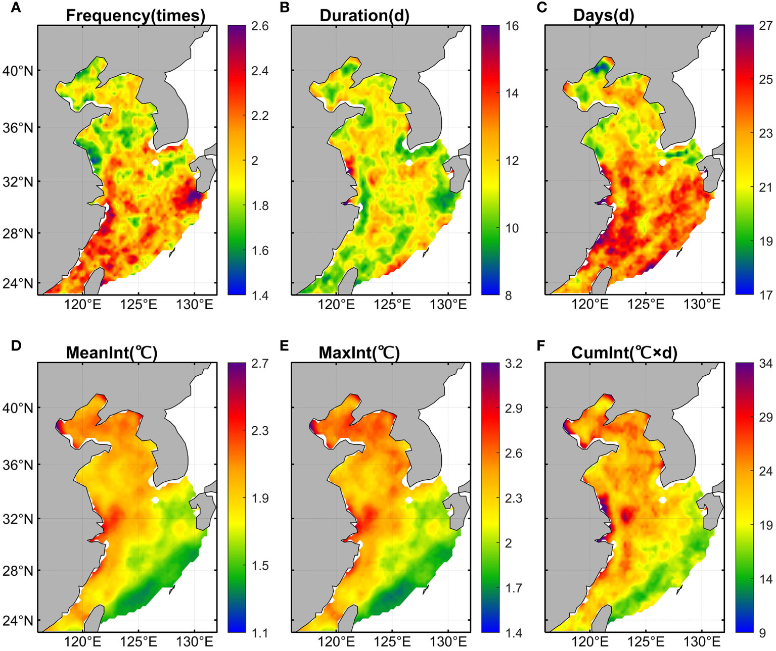
Figure 2 Spatial distributions of annual average MHWs’ (A) frequency, (B) duration, (C) days, and (D) MeanInt, (E) MaxInt, (F) CumInt in the ECMS during 1982-2022.

Figure 3 depicts the long-term trends of MHWs in the ECMS. With the exception of the eastern part of the YS, there is a significant positive growth trend in frequency, averaging 0.8 times/decade across the ECMS. This increase is more pronounced off the coast of China and in the ECS Kuroshio region, reaching a peak of 1.9 times/decade off northeast Taiwan (Figure 3A). Similarly, the duration of MHW events generally shows a positive trend, with an average increase of 1.3 days/decade, most notably in the central YS and ECS Kuroshio region, where the growth rate can reach up to 5.0 days/decade (Figure 3B). The combined effect of frequency and duration results in an overall positive trend in the annual average total days of MHW events, increasing by an average of 11.5 days/decade, especially in the western ECS and the Kuroshio, with a growth rate of exceeding 17.7 days/decade (Figure 3C). The long-term trends in MeanInt and MaxInt are 0.04°C/decade and 0.08°C/decade, respectively, in the entire ECMS. They show a similar spatial pattern: Most areas in the BS and YS display a positive trend, as well as around Taiwan, while a negative trend covers part areas in the ECS (Figures 3D, E). These results are consistent with those of Yao et al. (2020). CumInt mirrors the duration trend, showing an average growth of 2.9°C×days/decade, with the highest increase in the SYS region exceeding 15.6°C×days/decade (Figure 3F).

Figure 3

Figure 3 Long-term trends of MHWs from 1982 to 2022: (A) frequency, (B) duration, (C) days, (D) MeanInt, (E) MaxInt, (F) CumInt. The scattered regions indicate the areas where the trends are significant with a 95% confidence level.

By comparing with the annual mean value (Figure 2), it is observed that the MHW frequency is higher during summer, with duration and CumInt exceeding the annual average (Figure 4). Across the ECMS, the average frequency, duration, and total days of summer MHWs are 0.7 times, 11.5 days, and 7.4 days, respectively (Figures 4A–C). Higher-frequency MHWs occur near the coast of Zhejiang Province (27-31°N, 121-124°E), with peaks reaching 1.0 times. There is a negative spatial correlation (-0.63) between the frequency and duration of MHWs, with longer durations observed in the southwestern and southeastern SYS and offshore areas of the ECS. The total days of summer MHWs are relatively larger in the BS, YS and northern ECS, reaching 9.1 days. The MeanInt, MaxInt, and CumInt of summer MHWs are 1.9°C, 2.3°C, and 22.3°C×days, respectively (Figures 4D–F). MeanInt and MaxInt display significant north-south variations: north of 30°N, including the BS, YS, and northern ECS, the averages are higher at 2.3°C and 2.8°C; south of 30°N, these intensities are lower at 1.6°C and 2.0°C. The spatial distribution of CumInt, primarily influenced by MeanInt (spatial correlation coefficient between them is 0.82), also shows marked difference between the northern and southern regions, with average values of 26.8 and 19.9°C×days, respectively, across the 30°N divide. The highest CumInt value, exceeding 40°C×days, is recorded in the SYS.

Figure 4

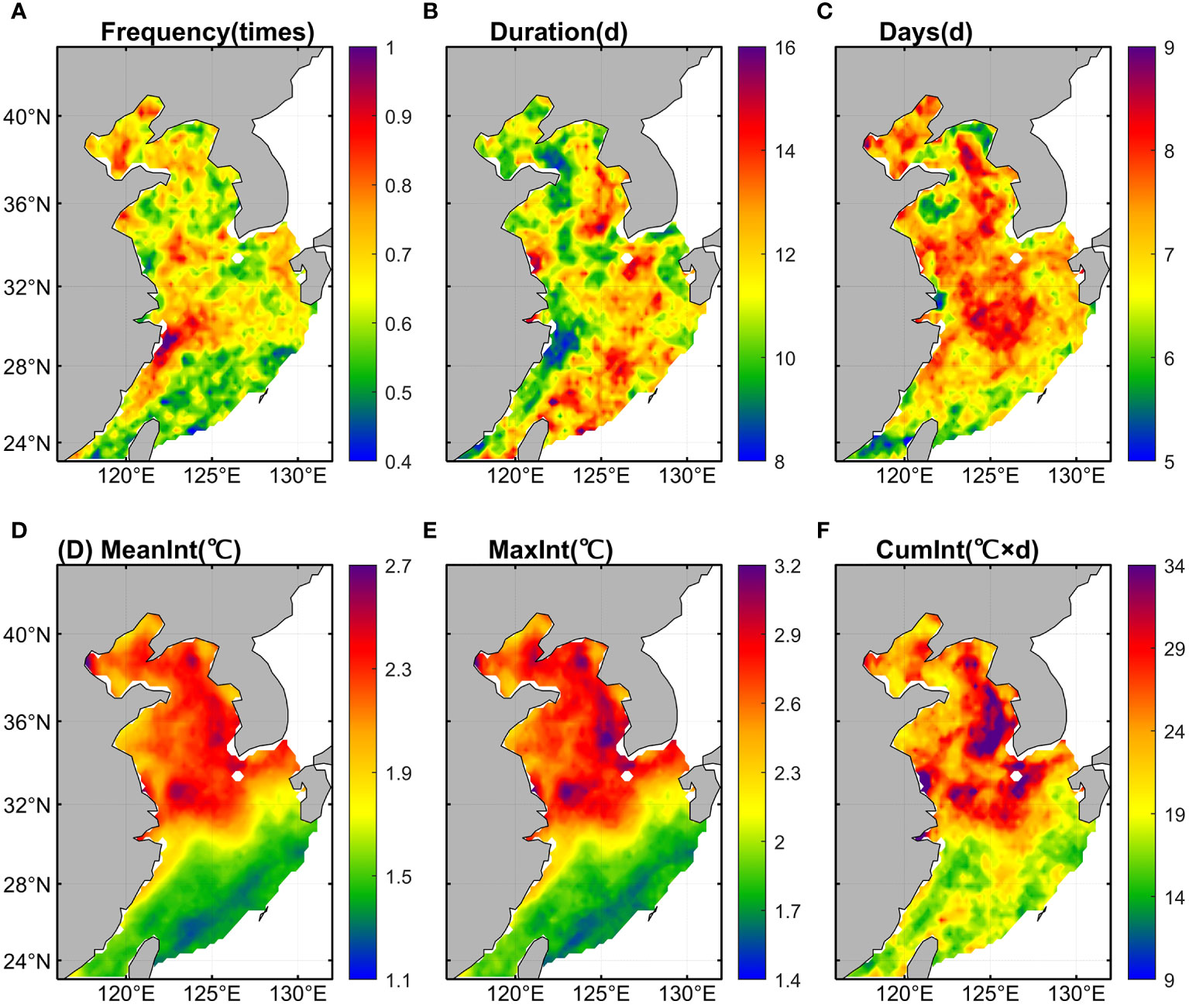
Figure 4 Spatial distributions of summer (JAS) average MHWs’ (A) frequency, (B) duration, (C) days, and (D) MeanInt, (E) MaxInt, (F) CumInt in the ECMS during 1982-2022.

In the context of global warming, an upward trend in the frequency and duration of summer MHW events in the ECMS is evident, with average increases of 0.3 times/decade and 2.1 days/decade, respectively (Figures 5A, B). The frequency of summer MHWs increases across most regions, barring the eastern portion of the YS, with higher growth rates along the coast of China. The most rapid increase in duration is observed in the SYS and southern ECS (south of 28°N), with the maximum growth rate exceeding 10.9 days/decade. Compared to the annual average increase in duration (1.3 days/decade), the trend in summer is more pronounced. The total days of MHWs, reflecting the combined effect of frequency and duration, primarily shows concentrated growth in the southwestern SYS and southern ECS, with the maximum growth rate exceeding 16.8 days/decade (Figure 5C). Compared with the results of Lee et al. (2023), there are some differences in the distribution of total days. The reason for the discrepancy is attributed to the different baseline period.

Figure 5

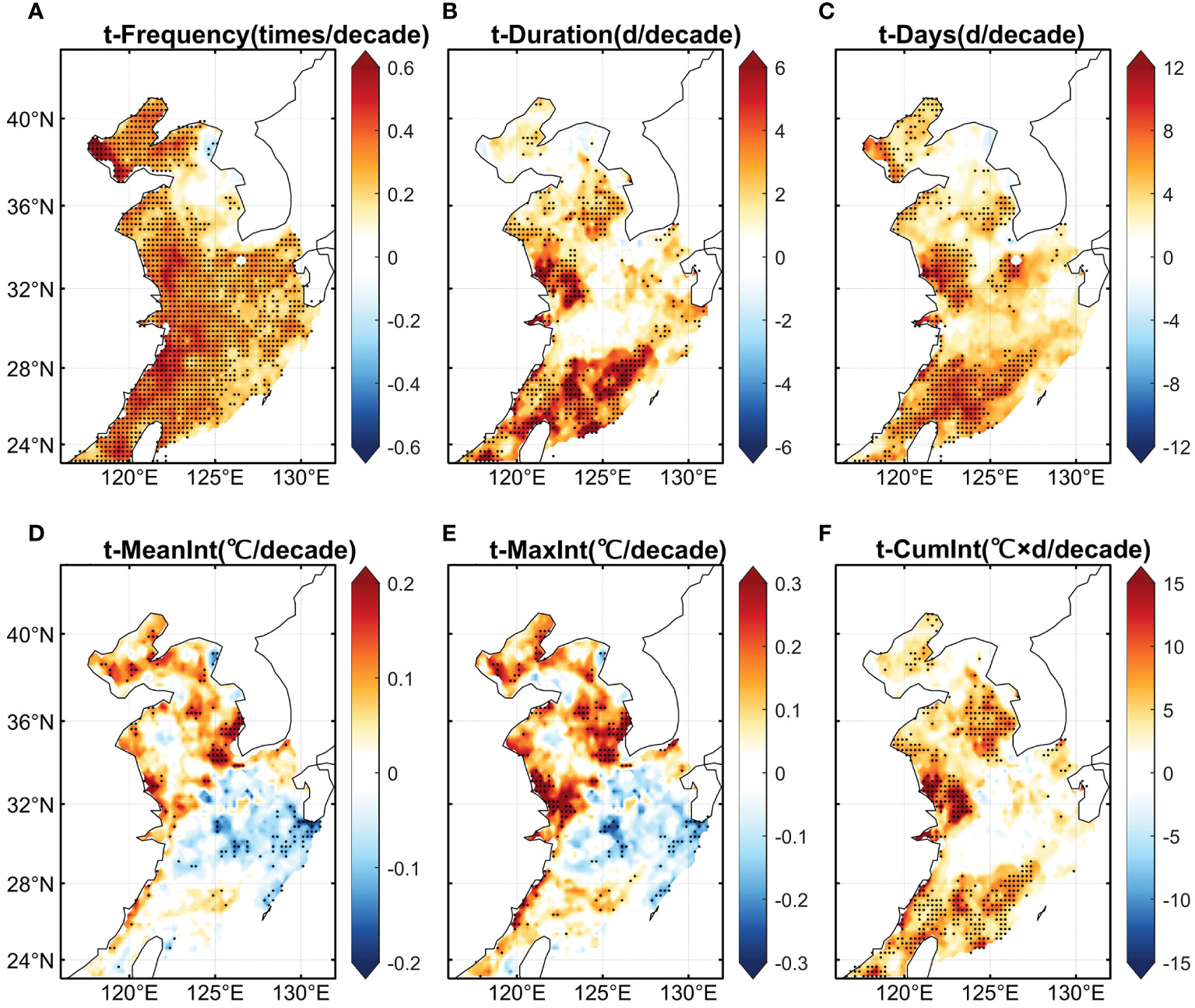
Figure 5 Long-term trends of MHWs during the summer from 1982 to 2022: (A) frequency, (B) duration, (C) days, (D) MeanInt, (E) MaxInt, (F) CumInt. The scattered regions indicate the areas where the trends are significant with a 95% confidence level.

Contrasting with frequency and duration, the long-term trends of MeanInt and MaxInt show both increases and decreases (Figures 5D, E). On the whole, the ECMS exhibits positive long-term trends in MeanInt and MaxInt, with values of 0.03°C/decade and 0.06°C/decade, respectively. Increasing trends are primarily observed in the BS and YS, with the former (BS) being at rates of 0.07°C/decade and 0.11°C/decade, and the latter (YS) being 0.15°C/decade and 0.23°C/decade, respectively, along with a slightly weaker upward trend in the southern ECS (south of 28°N). In contrast, the northern ECS (north of 28°N) displays decreasing trends, with rates of -0.06°C/decade and -0.08°C/decade. Compared to the annual average, the intensity changes of summer MHWs are more pronounced. Taking the SYS as an example, the annual increasing trend in MaxInt is 0.11°C/decade, while during summer, the rate escalates to 0.16°C/decade. Given the combined impact of duration and intensity, the CumInt primarily illustrates a positive growth trend across the ECMS, with an average increase of 5.8°C×days/decade, twice the annual average (Figure 5F). High-value areas are concentrated offshore of the Yangtze River Estuary, in the SYS and southern ECS, with peaks above 37°C×days/decade. The high values offshore of the Yangtze River Estuary and in the SYS result from the interplay of duration and intensity, while in the southern ECS, duration is the main factor.

3.1.2 EOF analysis

To elucidate the primary spatio-temporal features of summer MHWs in the ECMS, EOF analysis is conducted for CumInt. Figure 6 presents the first two principal modes of summer MHW CumInt, accounting for 59.11% and 9.53% of the total variance, respectively. In line with the North equation (North et al., 1982), these modes are fundamentally orthogonal. The first EOF mode of CumInt shows a uniform enhancement across the ECMS, most notably in the SYS and northern ECS (Figure 6A). The corresponding PC1 demonstrates an increasing trend, signifying a marked intensification of summer MHWs in the ECMS from 1982 to 2022 (Figure 6B). Moreover, PC1 exhibits significant interannual variability, with the most substantial increases occurring in 1994, 2016-2018, and 2021-2022. The strong 2016-2018 and 2022 MHWs in the SYS and northern ECS have been reported by Gao et al. (2020), Oh et al. (2023a), and Tan et al. (2023). The second EOF mode features a north-south dipole pattern, with positive signals in the BS and YS and negative signals across the ECS (Figure 6C). Its corresponding PC2 shows marked interannual fluctuations, peaking in 2018 (Figure 6D). The strong 2018 MHW event in the NYS has been investigated by Li et al. (2023). In contrast to PC1, the long-term trend in PC2 is insignificant.

Figure 6

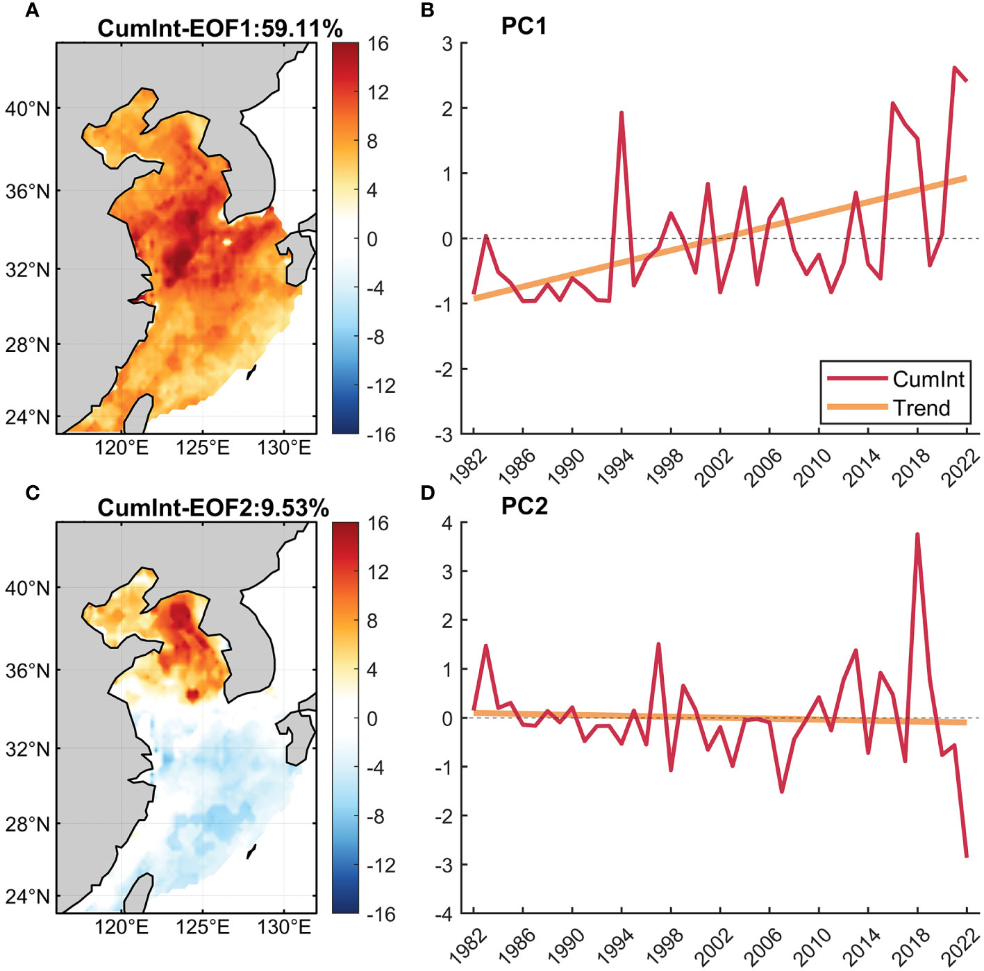
Figure 6 (A, C) Spatial patterns of the first two EOF modes of summer MHW CumInt in the ECMS and (B, D) the related PC time series. Solid lines represent linear trends.

Due to the close relationships between CumInt and duration as well as MeanInt, we performed EOF decompositions for both duration and MeanInt. The first mode of both variables show a positive anomaly across the entire ECMS, accounting for 60.96% and 65.26% of the total variances, respectively (Figures 7A, B). They both closely resemble the distribution of the first mode of CumInt, with spatial correlation coefficients of 0.75 and 0.89, respectively. Strong signals in duration are observed in the SYS and ECS, while larger values in MeanInt are found in the YS and northern ECS, both of which contribute significantly to the variation in CumInt, especially in the SYS and northern ECS. The corresponding PC1 of both variables exhibit similar long-term trends and interannual variations with CumInt as well, with correlation coefficients of 0.97 and 0.93, respectively (Figure 7C). The second mode of duration and MeanInt exhibit a dipole structure and interannual variations similar to CumInt (Figures 7D–F). The spatial correlation coefficients are 0.87 and 0.89, respectively, and the PC correlation coefficients are 0.90 and 0.81, respectively. Note that negative values in duration are mainly concentrated in the ECS Kuroshio region, while the negative anomalies in MeanInt are more pronounced offshore of the Yangtze River Estuary.

Figure 7

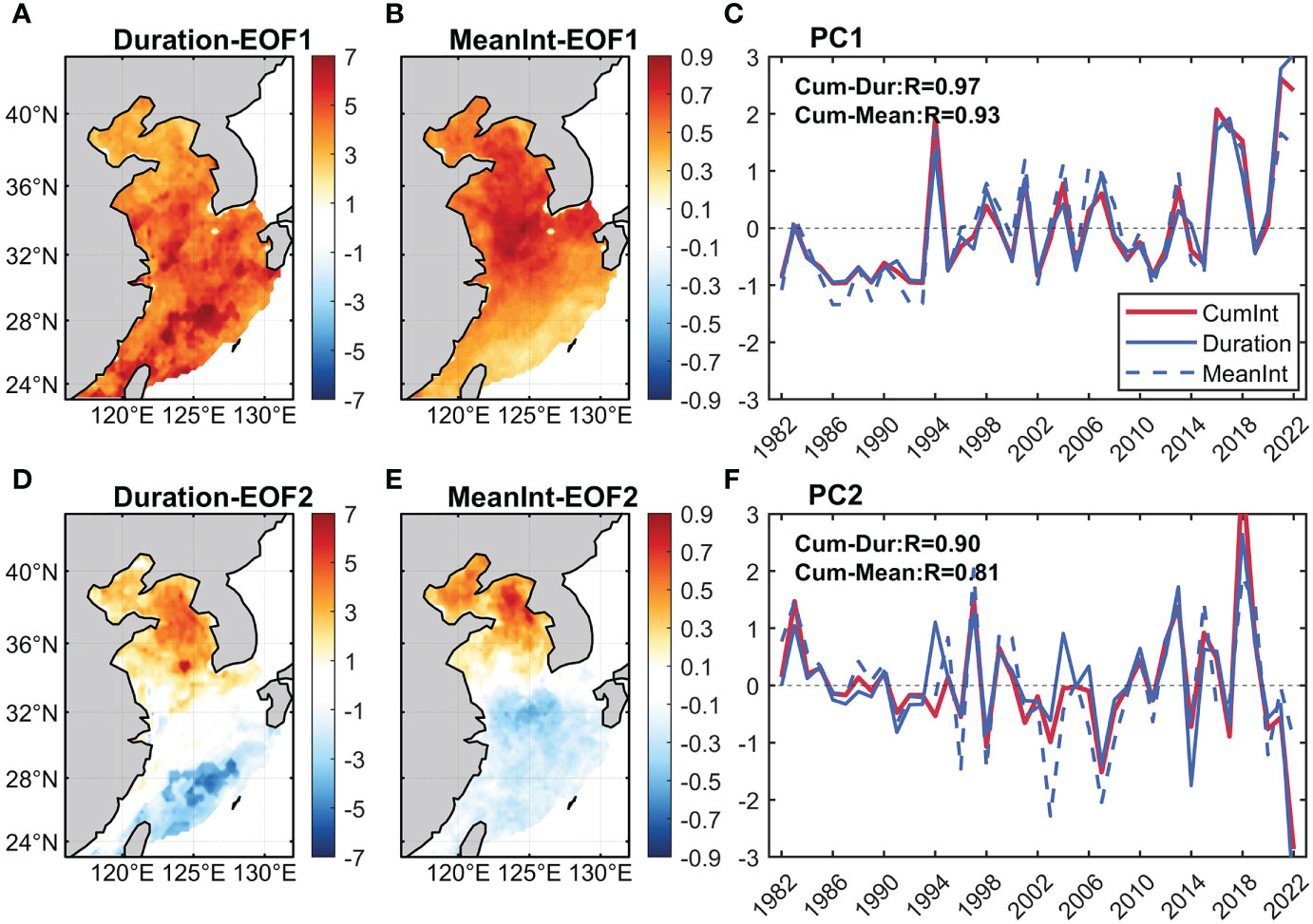
Figure 7 Spatial patterns of the first two EOF modes of summer MHW (A, D) duration and (B, E) MeanInt in the ECMS. (C, F) The related PC time series (solid and dashed blue curves). Red curves represent the PC time series of CumInt.

MHWs are defined as certain SST anomalies, which can be induced by increases/decreases in mean SST or changes in SST variance (Oliver, 2019). We conducted an EOF analysis on summer mean SST and SST variance in the ECMS (Figure 8). The first mode of summer mean SST accounts for 49.04% of the total variance, and the spatial distribution exhibits a high correlation with CumInt, with a spatial correlation coefficient of 0.73 (Figures 6A, 8A). The corresponding PC1 also exhibits a high correlation with that of CumInt (correlation coefficient is 0.87, Figure 8C). These findings indicate the change in summer mean SST is the main contributor in the long-term trends and interannual variations of CumInt. Notably, the change in summer SST variance also contributes to the long-term trend of CumInt in the YS (Figures 8B, C). The relative contribution between summer mean SST and SST variance needs to be evaluated in the future. The second mode of summer mean SST and SST variance contribute 17.03% and 16.41% of the total variance, respectively. The spatial distribution of both mean SST and SST variance is strongly correlated with CumInt, as evidenced by spatial correlation coefficients of 0.85 and 0.78, respectively (Figures 8D, E). The PC2 time series also show a moderate correlation with CumInt, with correlation coefficients of 0.61 and 0.53, respectively (Figure 8F). These results suggest that both mean SST and SST variability have important contributions to the interannual variations in this mode.

Figure 8

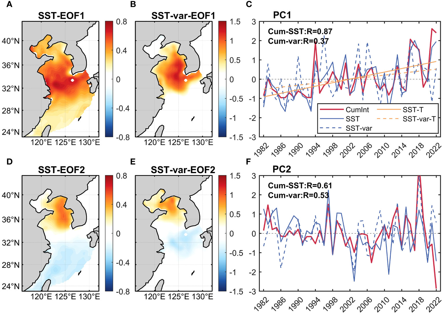
Figure 8 Spatial patterns of the first two EOF modes of summer (A, D) mean SST and (B, E) SST variance (SST-var) in the ECMS. (C, F) The related PC time series (solid and dashed blue curves). Red curves in (C, F) represent the PC time series of CumInt. Yellow lines in (C) represent the linear trends.

3.2 Extreme MHW events in summer

3.2.1 Classification and statistics of MHW events

Section 3.1 denotes an inclination for intense MHW events in the SYS, with a consistent upward trend in intensity from 1982 to 2022 (Figures 5, 7). Indeed, a recent surge in extreme MHW events in the SYS has been reported (Gao et al., 2020; Yan et al., 2020; Li et al., 2022, Li et al., 2023; Tan et al., 2023; Oh et al., 2023a). To delve deeper into the extreme MHW events in the SYS, we treated the SYS collectively and detected MHW events during summer. The findings reveal a total of 29 MHW events in the SYS during summer, with over 40% of these events transpiring in the last decade (2013-2022) displaying MeanInt and MaxInt of 1.80°C and 3.23°C (Figure 9A). The intensity of these events significantly surpasses that of the earlier period (1982-2012).

Figure 9

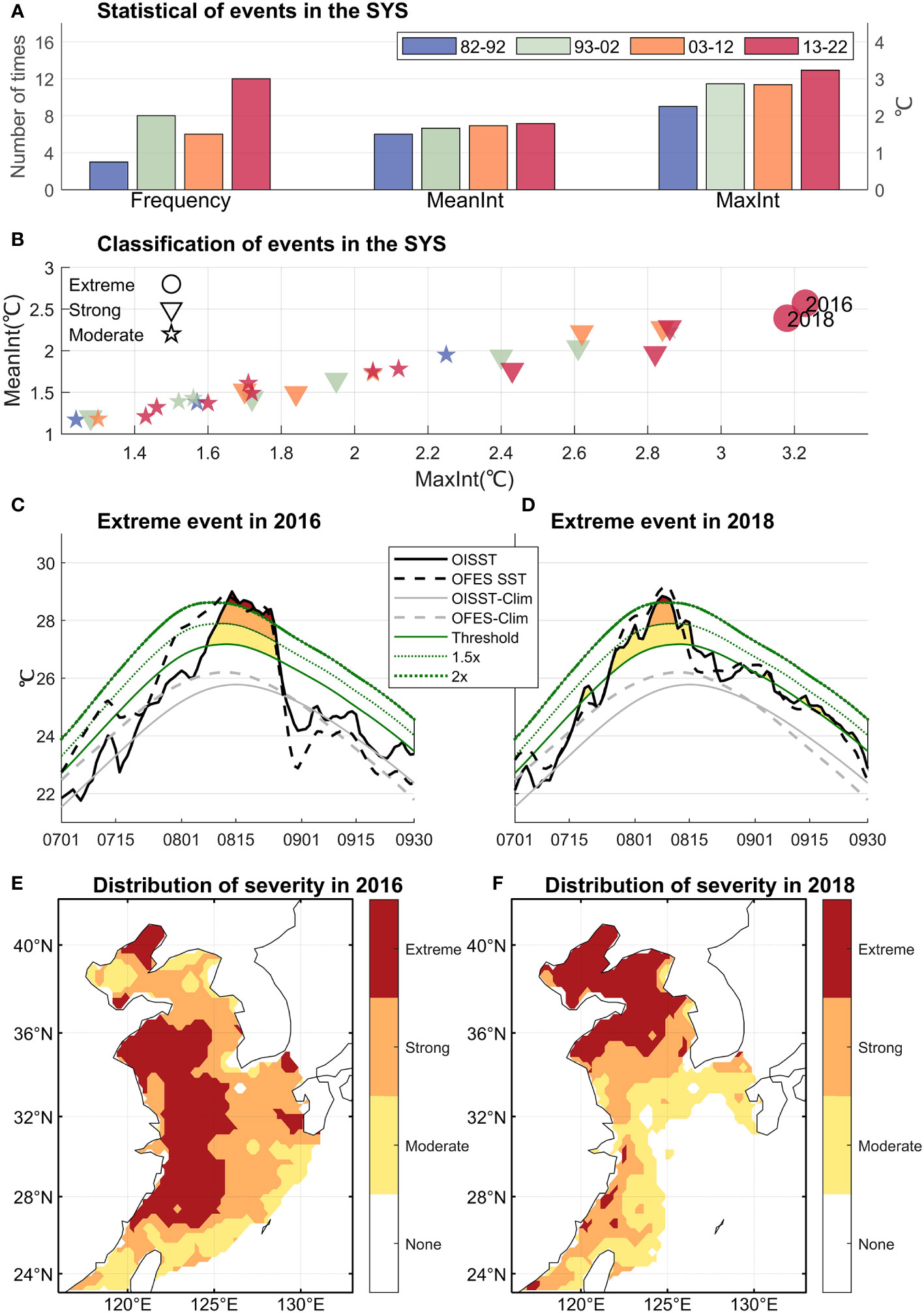
Figure 9 (A, B) Statistical and classification of summer MHW events in the SYS. (C, D) Extreme MHW events in 2016 and 2018 and (E, F) their severity distribution.

Expanding upon prior research (Hobday et al., 2018; Oliver et al., 2019), we categorized summer MHW events in the SYS into three distinct groups: Extreme events, Strong events and Moderate events (Figure 9B). It is found that Extreme MHWs transpired in 2016 and 2018. In particular, the 2016 Extreme MHW stands out with the longest duration at the extreme level, marked by an extreme high temperature persisting for 12 days (Figures 9C, D). Following the categorization of each grid point in the ECMS during Extreme event periods, the 2016 Extreme event was characterized by a broadscale occurrence in both the southwestern SYS and northwestern ECS (Figure 9E). On the other hand, the 2018 event predominantly occurred in the BS, NYS and northern SYS (Figure 9F). The distributions of these Extreme events align with the spatial patterns and significant years of the first and second modes of the EOF, as detailed in Section 3.1.2 (Figures 6–8).

3.2.2 Mechanism of Extreme MHW events

To discern the primary determinants influencing Extreme MHW events, we undertook a diagnostic analysis of the MLT equation using OFES data. Yan et al. (2020) have confirmed that OFES can reproduce the ML dynamics and accurately replicate extreme SST variations in the SYS and northern ECS. We further validated the proficiency of OFES in simulating the SYS SST by assessing its performance during 2016 and 2018. The results showed that OFES precisely mirrored SST variations (Figures 9C, D).

Figure 10 illustrates the climatology of each term in the MLT equation in the SYS. It is clear that the horizontal advection term contributes minimally during summer, while the MLT tendency term is primarily governed by the net heat flux term and the vertical entrainment term. Figure 11 displays anomalies of the terms for 2016 and 2018 compared to the climatology. Positive anomalies in the MLT tendency term signify that the MLT increases more rapidly or decreases more slowly than the climatology. The positive anomalies of the MLT tendency term during the periods from July 22 to August 14, 2016 and from July 25 to August 12, 2018, highlighted in shaded areas, were responsible for the generation of the Extreme MHW events in 2016 and 2018. During these two periods, the anomaly in the horizontal advection term was negligible, indicating its minimal contribution. The positive anomaly in the MLT tendency term predominantly resulted from anomalies in the surface heat flux term and the vertical entrainment term.

Figure 10

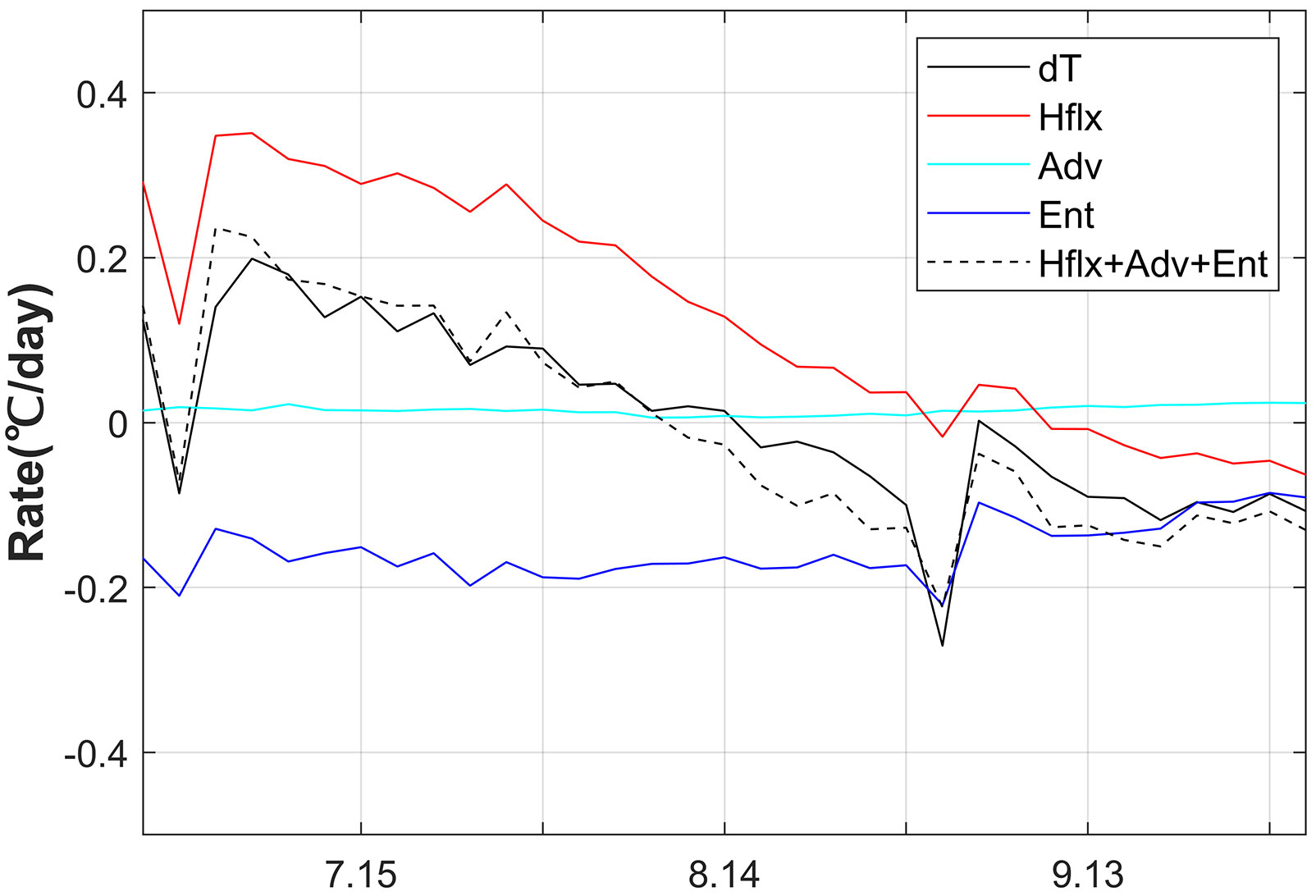
Figure 10 All the terms in the MLT equation over the SYS calculated from the OFES outputs: the MLT tendency term (dT), the surface heat flux term (Hflx), the horizontal advection term (Adv), and the vertical entrainment term (Ent), and the sum of the surface heat flux term, the horizontal advection term, and the vertical entrainment term (Hflx+Adv+Ent).

Figure 11

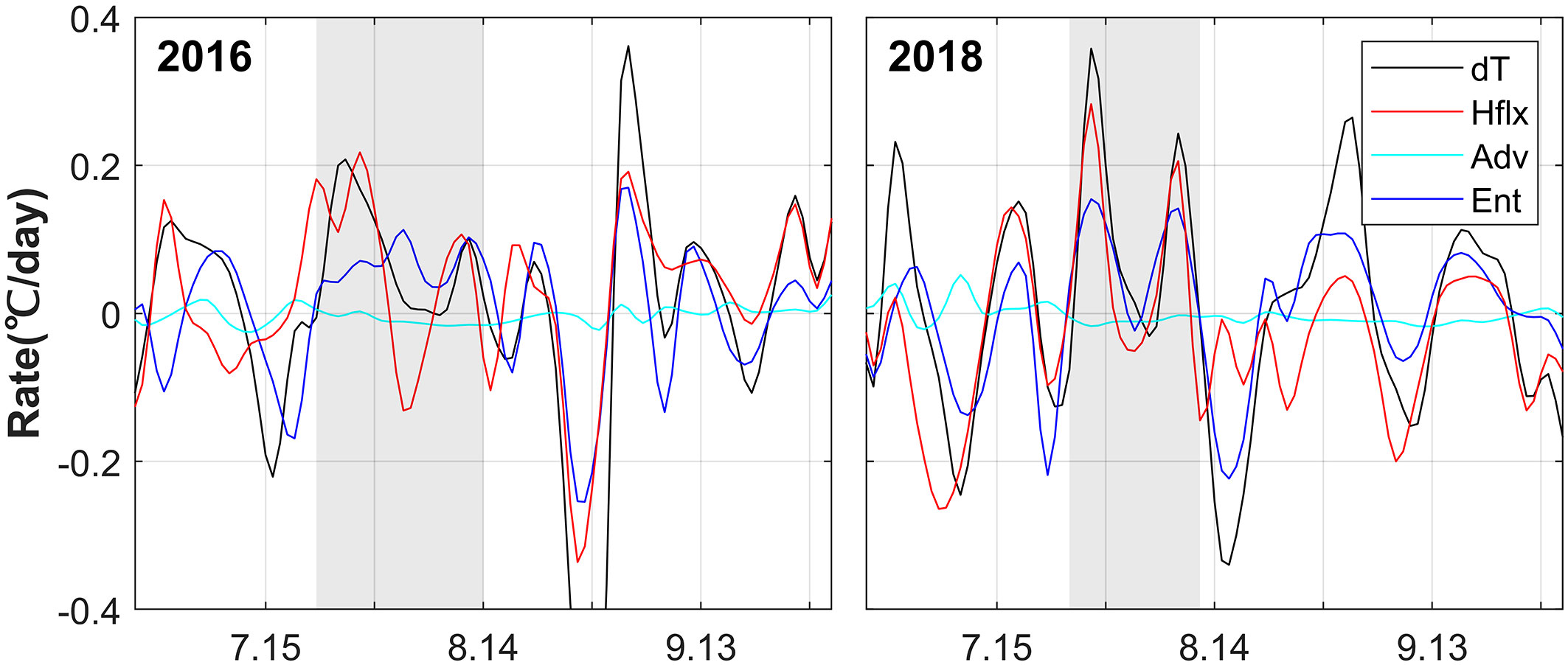
Figure 11 Anomalies of all the terms in the MLT equation in 2016 and 2018, relative to the daily climatology calculated from the OFES outputs.

A comprehensive analysis of shortwave radiation, wind speed, and MLD during warming periods in 2016 and 2018 is depicted in Figure 12. In 2016, during the early warming phase, shortwave radiation significantly increased, followed by a sharp decline and subsequent rise. Meanwhile, wind speed and MLD transitioned from positive anomalies to negative anomalies. The increased shortwave radiation and reduced wind speed stabilized the upper ocean and suppressed oceanic turbulent mixing, reflected by a negative MLD anomaly, resulting in the positive anomalies in the surface heat flux term and the vertical entrainment term, and therefore leading to anomalous warming. A similar situation arose in 2018.

Figure 12

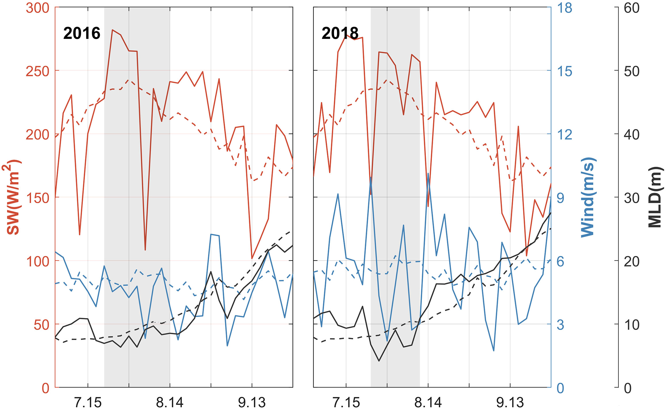
Figure 12 Shortwave radiation (solid red curve), surface wind speed (solid blue curve) and mixed layer depth (MLD, solid black curve) during the Extreme MHW event in 2016 and 2018. Dashed line represents the climatology.

Figure 13 depicts composite maps of 500-hPa geopotential height and associated atmospheric variables during the anomalous warming periods of 2016 and 2018. The results reveal that during the anomalous warming period, the SYS was influenced by an anomalous high-pressure system, which split from the western Pacific subtropical high. This resulted in subsidence over the SYS region, triggering a decrease in surface winds. Additionally, the subsidence bolstered atmospheric stability, inhibiting cloud formation and amplifying solar radiation at the sea surface. For instance, during the anomalous warming period of 2016, the entire SYS was under the influence of a high-pressure system. This corresponded to a decline in wind speed, diminished cloud cover, and a shortwave radiation increment of roughly 20 W/m², contributing to a persistent increase in SST (Figures 13A, B). In 2018, during the analogous anomalous warming period, the high-pressure system over the SYS led to localized wind speed reduction, decreased cloud cover, and a significant surge in shortwave radiation, with a maximum positive anomaly exceeding 40 W/m² (Figures 13C, D). This culminated in a localized extreme heat in the SYS.

Figure 13

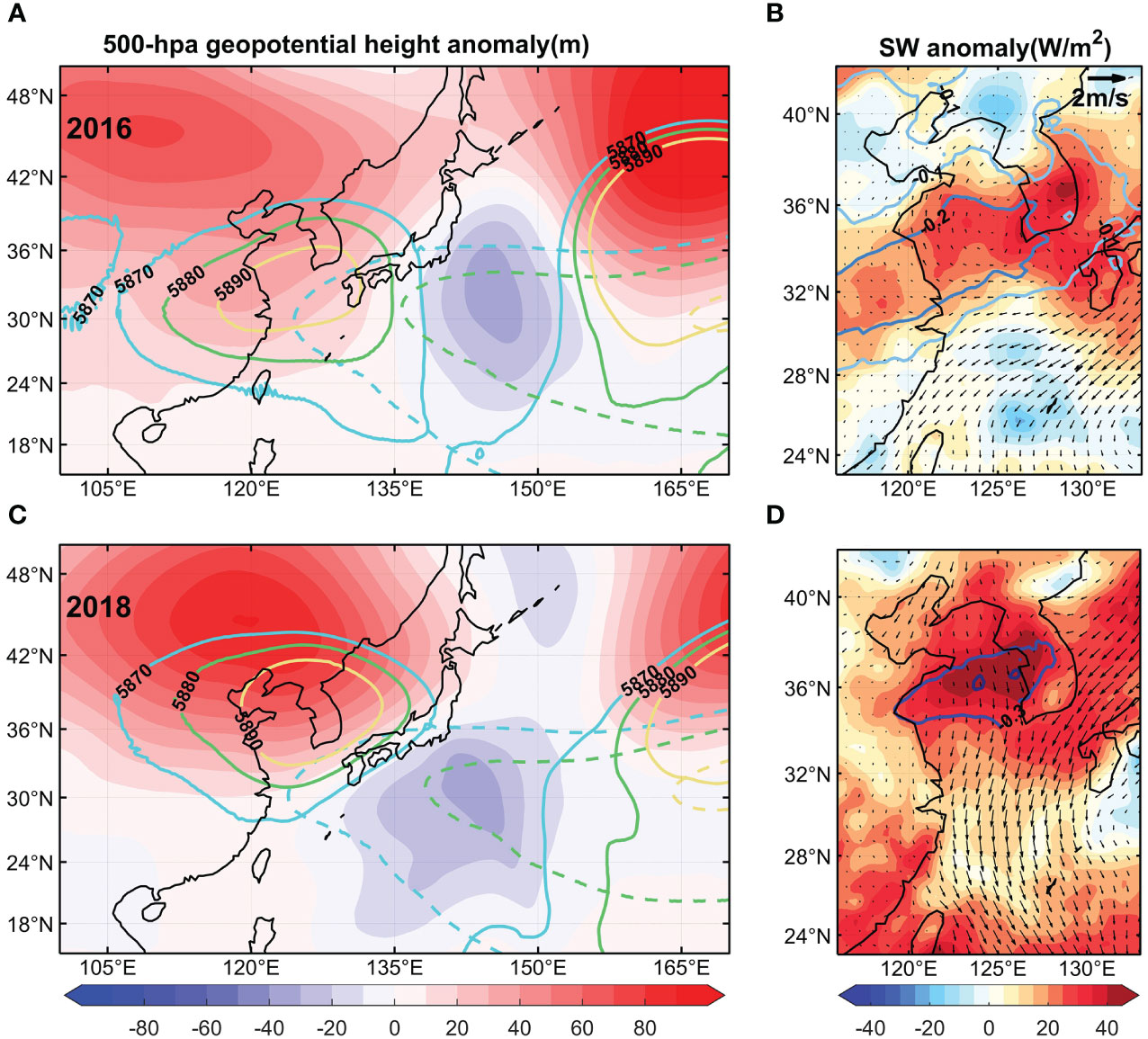
Figure 13 (A, C) Anomalies of 500-hpa geopotential height (shading) during the period of the anomalous SST rise in 2016 and 2018. The solid and dashed contours denote 500-hpa geopotential height and its climatology. (B, D) Anomalies of shortwave radiation (shading), wind fields at the sea surface (arrow), and cloud fraction (contours) during the period.

In short, the Extreme MHW events in 2016 and 2018 were associated with anomalous high-pressure system over the SYS splitting from the western Pacific subtropical high. The high-pressure anomaly induced an enhancement in surface solar radiation and a reduction in surface wind speed, both of which stabilized the upper ocean and suppressed oceanic turbulent mixing, causing more heat concentrating near the sea surface and forming Extreme MHWs. The formation mechanism for the Extreme MHW events in the SYS agrees with that for the record-breaking SST reported by Yan et al. (2020). Choi et al. (2022) also suggested that the northwestward expanding subtropical high was closely related to the occurrence of MHWs in summer, but they only discussed the atmospheric changes associated with the anomalous subtropical high, not considered the relevant oceanic changes.

4 Summary and discussion

Under the context of global warming, the frequency of MHWs in the ECMS has markedly increased (Li et al., 2019; Wang et al., 2019; Yao et al., 2020; Choi et al., 2022; Oh et al., 2023b). Especially in recent years, more extreme MHW events during summer have become increasingly common (Tan and Cai, 2018; Wang et al., 2019; Li et al., 2023; Tan et al., 2023; Oh et al., 2023a), exerting significant impacts on the ecosystems and fisheries in the ECMS. This study utilized OISST satellite data and OFES model data to examine the long-term trends of summer MHWs in the ECMS and to explore the underlying contributing factors of the Extreme MHW events in 2016 and 2018. The key findings are summarized as follows:

(1) The frequency of summer MHWs across most parts of the ECMS has seen an increase, exhibiting a higher growth rate along the China coast. Areas experiencing a more rapid increase in duration are primarily situated in the SYS and southern ECS (south of 28°N). The long-term trends of MeanInt and MaxInt display varied patterns across different regions: A notable increasing trend is observed in the BS and YS, whereas a decreasing trend is evident in the northern ECS (north of 28°N). Due to the combined effects of duration and intensity, the CumInt in the ECMS demonstrates a generally positive trend, with peak values concentrated offshore of the Yangtze River Estuary, in the SYS and southern ECS.

(2) The primary mode of CumInt highlights a pronounced long-term increasing trend and significant interannual variations across the entire ECMS, especially notable in the SYS and northern ECS, which are predominantly influenced by summer mean SST warming. Additionally, change in summer SST variance also contributes to the long-term increasing trend in the YS. The secondary mode of EOF analysis reveals a north-south dipole pattern, with its interannual variations being driven by the combined effects of changes in both summer mean SST and SST variance.

(3) Extreme MHW events in 2016 and 2018 were primarily associated with the surface heat flux term and the vertical entrainment term, while the horizontal advection term exerted a relatively minor influence. The manifestation of these Extreme MHW events was mainly connected to the high-pressure system over the SYS, which split from the western Pacific subtropical high. Under the sway of this high-pressure system, atmospheric stability escalated, thereby inhibiting cloud formation. Consequently, shortwave radiation increased, sea surface wind speed decreased, and oceanic turbulence reduced. This sequence of events resulted in an accumulation of heat near the sea surface, which raised the SST and caused the occurrence of Extreme MHW events.

In this study, we continued to use the widely classification method based on intensity (Hobday et al., 2018; Oliver et al., 2019) for classifying MHW. However, it’s possible that MHWs appearing over a longer period with moderate intensity might have a greater impact on marine environments compared to those with short durations but high intensity. CumInt, considering both intensity and duration, is a reasonable parameter to classify MHW. Based on CumInt, the three strongest MHWs in the SYS occurred in 2017, 2018, and 2016. The strongest MHW event in 2017 was due to its longest duration. When studying the mechanism of the longest event in 2017, it was discovered to consist of two warming periods: one period at the turn of spring and summer (from June 15 to July 6) and the other in summer (from July 18 to July 28, Supplementary Figure S2A). At the turn of spring and summer, MHW occurred in the BS, NYS, and northern SYS, while it occurred in the SYS and ECS during summer (Supplementary Figures S2B, C). Synthesized maps showed that at the turn of spring and summer, the MHW in the BS, NYS, and northern SYS was not related to the western Pacific high located between 15°N-25°N (Figure 14A, B), while the MHW during summer was associated with the split of the western Pacific high (Figure 14C, D), consistent with MHWs in 2016 and 2018. In this study, we focus on summer MHW. For MHW in 2017, when only the period in summer is considered, its CumInt is smaller than that in 2016 and 2018. Therefore, when using CumInt as the parameter to classify MHW, the two strongest MHWs still occurred in 2016 and 2018.

Figure 14

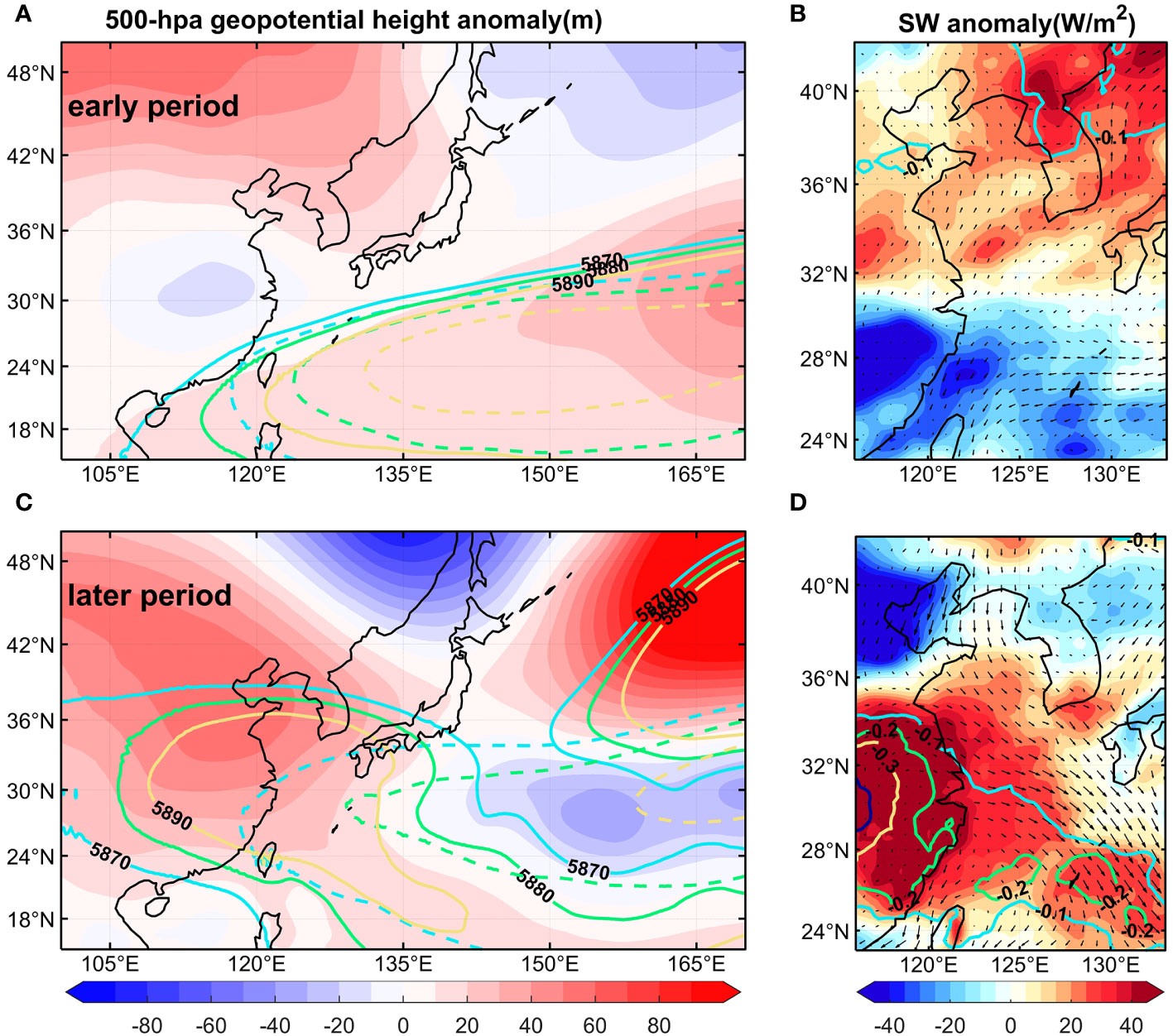
Figure 14 Anomalies of (A) 500-hpa geopotential height (shading) and (B) shortwave radiation (shading), wind fields at the sea surface (arrow), and cloud fraction (contours) at the turn of spring and summer in 2017 (June 15 to July 6). (C, D) is the same as (A, B) except for summer (from July 18 to July 28). The solid and dashed contours in (A, C) denote 500-hpa geopotential height and its climatology.

Our results suggested that the reduced oceanic turbulent mixing (decreased MLD) was important for the generation of the Extreme MHWs in 2016 and 2018. Previous studies have shown that the diluted freshwater from the Yangtze River may form a shallow MLD by producing salt stratification above the top of the thermocline (Sprintall and Tomczak, 1992; Belkin, 2009; Moon et al., 2019; Tak et al., 2023). Therefore, the Yangtze River freshwater may contribute to anomalous SST rises or MHWs, for example, in summer 2016 and 2022 (Moon et al., 2019; Yan et al., 2020; Oh et al., 2023a). Tides is another factor influencing the oceanic mixing and SST (Kim et al., 2010; Meng et al., 2020; Lee et al., 2022b), which may also contribute to MHWs. Quantitative assessment of the contribution of Yangtze River freshwater and tides is needed in the future.

In contrast to our conclusion, Gao et al. (2020) suggested that the ocean advection anomalies also contributed significantly to the extreme MHW in 2018. Their numerical results using FVCOM (Finite Volume Community Ocean Model) showed that upper ocean heat was transported into the SYS, accumulated in an anticyclone eddy. While the reason for the difference in the role of ocean advection is not clear, a possible explanation is that the simulated current field in the OFES is different from that in the FVCOM.

Data availability statement

The original contributions presented in the study are included in the article/Supplementary Material. Further inquiries can be directed to the corresponding author.

Author contributions

JX: Writing – original draft, Data curation, Formal analysis, Investigation, Methodology, Software, Validation, Visualization, Writing – review & editing, Resources. YWY: Conceptualization, Formal analysis, Funding acquisition, Investigation, Methodology, Project administration, Resources, Supervision, Validation, Writing – review & editing. LZ: Funding acquisition, Supervision, Validation, Writing – review & editing, Methodology. WX: Funding acquisition, Supervision, Validation, Writing – review & editing. LM: Methodology, Software, Writing – review & editing. YY: Funding acquisition, Software, Supervision, Writing – review & editing. CC: Funding acquisition, Supervision, Writing – review & editing.

Funding

The author(s) declare that financial support was received for the research, authorship, and/or publication of this article. YY is supported by Southern Marine Science and Engineering Guangdong Laboratory (Zhuhai) (SML2023SP219) and Zhejiang Provincial Natural Science Foundation of China (LY23D060006). YWY is supported by the National Natural Science Foundation of China (42376002). LZ is supported by the development fund of South China Sea Institute of Oceanology of the Chinese Academy of Sciences SCSIO202203. WX is supported by the National Key R&D Program of China: Young Scientist Program (2023YFC3108800).

Acknowledgments

The authors would like to express gratitude to the NOAA for providing the OISST v2 dataset (https://downloads.psl.noaa.gov/). The authors would like to acknowledge the APDRC for furnishing the OFES outputs dataset (http://apdrc.soest.hawaii.edu/) and the ECMWF for providing the ERA5 dataset (https://cds.climate.copernicus.eu/). The authors also acknowledge the authors of Hobday et al. (2016) who generously provided access to their numerical codes (https://github.com/ecjoliver/marineHeatWaves) for computing the set of MHW metrics. Furthermore, the authors thank for Key Laboratory of Polar Atmosphere-ocean-ice System for Weather and Climate, Ministry of Education funding the study. At last, the authors are grateful to anonymous reviewers for their invaluable feedback on this manuscript.

Conflict of interest

The authors declare that the research was conducted in the absence of any commercial or financial relationships that could be construed as a potential conflict of interest.

Publisher’s note

All claims expressed in this article are solely those of the authors and do not necessarily represent those of their affiliated organizations, or those of the publisher, the editors and the reviewers. Any product that may be evaluated in this article, or claim that may be made by its manufacturer, is not guaranteed or endorsed by the publisher.

Supplementary material

The Supplementary Material for this article can be found online at: https://www.frontiersin.org/articles/10.3389/fmars.2024.1380963/full#supplementary-material

References

Amaya D. J., Miller A. J., Xie S. P., Kosaka Y. (2020). Physical drivers of the summer 2019 North Pacific marine heatwave. Nat. Commun. 11, 1903. doi: 10.1038/s41467-020-15820-w

PubMed Abstract | CrossRef Full Text | Google Scholar

Bao B., Ren G. (2014). Climatological characteristics and long-term change of SST over the marginal seas of China. Cont. Shelf Res. 77, 96–106. doi: 10.1016/j.csr.2014.01.013

CrossRef Full Text | Google Scholar

Belkin I. M. (2009). Rapid warming of large marine ecosystems. Prog. Oceanogr. 81, 207–213. doi: 10.1016/j.pocean.2009.04.011

CrossRef Full Text | Google Scholar

Caputi N., Kangas M., Denham A., Feng M., Pearce A., Hetzel Y., et al. (2016). Management adaptation of invertebrate fisheries to an extreme marine heat wave event at a global warming hot spot. Ecol. Evol. 6, 3583–3593. doi: 10.1002/ece3.2137

PubMed Abstract | CrossRef Full Text | Google Scholar

Cheng Y., Zhang M., Song Z., Wang G., Zhao C., Shu Q., et al. (2023). A quantitative analysis of marine heatwaves in response to rising sea surface temperature. Sci. Total Environ. 881, 163396. doi: 10.1016/j.scitotenv.2023.163396

PubMed Abstract | CrossRef Full Text | Google Scholar

Cheung W. W., Frölicher T. L. (2020). Marine heatwaves exacerbate climate change impacts for fisheries in the northeast Pacific. Sci. Rep. 10, 6678. doi: 10.1038/s41598-020-63650-z

PubMed Abstract | CrossRef Full Text | Google Scholar

Choi W., Bang M., Joh Y., Ham Y.-G., Kang N., Jang C. J. (2022). Characteristics and mechanisms of marine heatwaves in the East Asian marginal seas: regional and seasonal differences. Remote Sens. 14, 3522. doi: 10.3390/rs14153522

CrossRef Full Text | Google Scholar

Feng M., McPhaden M. J., Xie S. P., Hafner J. (2013). La Niña forces unprecedented Leeuwin Current warming in 2011. Sci. Rep. 3, 1277. doi: 10.1038/srep01277

PubMed Abstract | CrossRef Full Text | Google Scholar

Frölicher T. L., Fischer E. M., Gruber N. (2018). Marine heatwaves under global warming. Nature 560, 360–364. doi: 10.1038/s41586-018-0383-9

PubMed Abstract | CrossRef Full Text | Google Scholar

Frölicher T. L., Laufkötter C. (2018). Emerging risks from marine heat waves. Nat. Commun. 9, 650. doi: 10.1038/s41467-018-03163-6

PubMed Abstract | CrossRef Full Text | Google Scholar

Gao G., Marin M., Feng M., Yin B., Yang D., Feng X., et al. (2020). Drivers of marine heatwaves in the East China Sea and the South Yellow Sea in three consecutive summers during 2016–2018. J. Geophys. Res. Oceans. 125, e2020JC01651. doi: 10.1029/2020JC016518

CrossRef Full Text | Google Scholar

Garrabou J., Coma R., Bensoussan N., Bally M., Chevaldonnè P., Clgliano M., et al. (2009). Mass mortality in Northwestern Mediterranean rocky benthic communities: Effects of the 2003 heat wave. Glob. Change Biol. 15, 1090–1103. doi: 10.1111/j.1365-2486.2008.01823.x

CrossRef Full Text | Google Scholar

Garrabou J., Gómez-Gras D., Medrano A., Cerrano C., Ponti M., Schlegel R., et al. (2022). Marine heatwaves drive recurrent mass mortalities in the Mediterranean Sea. Glob. Change Biol. 28, 5708–5725. doi: 10.1111/gcb.16301

CrossRef Full Text | Google Scholar

Genevier L. G., Jamil T., Raitsos D. E., Krokos G., Hoteit I. (2019). Marine heatwaves reveal coral reef zones susceptible to bleaching in the Red Sea. Glob. Change Biol. 25, 2338–2351. doi: 10.1111/gcb.14652

CrossRef Full Text | Google Scholar

Hayashida H., Matear R. J., Strutton P. G., Zhang X. (2020). Insights into projected changes in marine heatwaves from a high-resolution ocean circulation model. Nat. Commun. 11, 4352. doi: 10.1038/s41467-020-18241-x

PubMed Abstract | CrossRef Full Text | Google Scholar

Hersbach H., Bell B., Berrisford P., Hirahara S., Horányi A., Muñoz-Sabater J., et al. (2020). The ERA5 global reanalysis. Q. J. R. Meteorol. Soc 146, 1999–2049. doi: 10.1002/qj.3803

CrossRef Full Text | Google Scholar

Hobday A. J., Alexander L. V., Perkins S. E., Smale D. A., Straub S. C., Oliver E. C., et al. (2016). A hierarchical approach to defining marine heatwaves. Prog. Oceanogr. 141, 227–238. doi: 10.1016/j.pocean.2015.12.014

CrossRef Full Text | Google Scholar

Hobday A. J., Oliver E. C., Gupta A. S., Benthuysen J. A., Burrows M. T., Donat M. G., et al. (2018). Categorizing and naming marine heatwaves. Oceanography 31, 162–173. doi: 10.5670/oceanog.2018.205

CrossRef Full Text | Google Scholar

Hobday A. J., Pecl G. T. (2014). Identification of global marine hotspots: sentinels for change and vanguards for adaptation action. Rev. Fish Biol. Fish. 24, 415–425. doi: 10.1007/s11160-013-9326-6

CrossRef Full Text | Google Scholar

Holbrook N. J., Hernaman V., Koshiba S., Lako J., Kajtar J. B., Amosa P., et al. (2021). Impacts of marine heatwaves on tropical western and central Pacific Island nations and their communities. Global Planet. Change. 208, 103680. doi: 10.1016/j.gloplacha.2021.103680

CrossRef Full Text | Google Scholar

Holbrook N. J., Scannell H. A., Sen Gupta A., Benthuysen J. A., Feng M., Oliver E. C., et al. (2019). A global assessment of marine heatwaves and their drivers. Nat. Commun. 10, 2624. doi: 10.1038/s41467-019-10206-z

PubMed Abstract | CrossRef Full Text | Google Scholar

Holbrook N. J., Sen Gupta A., Oliver E. C., Hobday A. J., Benthuysen J. A., Scannell H. A., et al. (2020). Keeping pace with marine heatwaves. Nat. Rev. Earth Environ. 1, 482–493. doi: 10.1038/s43017-020-0068-4

CrossRef Full Text | Google Scholar

Huang B., Liu C., Freeman E., Graham G., Smith T., Zhang H. M. (2021). Assessment and intercomparison of NOAA daily optimum interpolation sea surface temperature (DOISST) version 2.1. J. Climate. 34, 7421–7441. doi: 10.1175/JCLI-D-21-0001.1

CrossRef Full Text | Google Scholar

Hughes T. P., Kerry J. T., Álvarez-Noriega M., Álvarez-Romero J. G., Anderson K. D., Baird A. H., et al. (2017). Global warming and recurrent mass bleaching of corals. Nature 543, 373–377. doi: 10.1038/nature21707

PubMed Abstract | CrossRef Full Text | Google Scholar

Jacox M. G. (2019). Marine heatwaves in a changing climate. Nature 571, 485e487. doi: 10.1038/d41586-019-02196-1

CrossRef Full Text | Google Scholar

Jacox M. G., Alexander M. A., Amaya D., Becker E., Bograd S. J., Brodie S., et al. (2022). Global seasonal forecasts of marine heatwaves. Nature 604, 486–490. doi: 10.1038/s41586-022-04573-9

PubMed Abstract | CrossRef Full Text | Google Scholar

Kim T. W., Cho Y. K., You K. W., Jung K. T. (2010). Effect of tidal flat on seawater temperature variation in the southwest coast of Korea. J. Geophys. Res. Oceans. 115(C2). doi: 10.1029/2009JC005593

CrossRef Full Text | Google Scholar

Laufkötter C., Zscheischler J., Frölicher T. L. (2020). High-impact marine heatwaves attributable to human-induced global warming. Science 369, 1621–1625. doi: 10.1126/science.aba0690

PubMed Abstract | CrossRef Full Text | Google Scholar

Lee S. T., Cho Y. K., Kim D. J. (2022b). Immense variability in the sea surface temperature near macro tidal flat revealed by high-resolution satellite data (Landsat 8). Sci. Rep. 12, 1–8. doi: 10.1038/s41598-021-04465-4

PubMed Abstract | CrossRef Full Text | Google Scholar

Lee S., Park M. S., Kwon M., Kim Y. H., Park Y. G. (2020). Two major modes of East Asian marine heatwaves. Environ. Res. Lett. 15, 074008. doi: 10.1088/1748-9326/ab8527

CrossRef Full Text | Google Scholar

Lee S., Park M. S., Kwon M., Park Y. G., Kim Y. H., Choi N. (2023). Rapidly changing East Asian marine heatwaves under a warming climate. J. Geophys. Res. Oceans. 128, e2023JC019761. doi: 10.1029/2023JC019761

CrossRef Full Text | Google Scholar

Lee S. B., Yeh S. W., Lee J. S., Park Y. G., Kwon M., Jun S. Y., et al. (2022a). Roles of atmosphere thermodynamic and ocean dynamic processes on the upward trend of summer marine heatwaves occurrence in East Asian marginal seas. Front. Mar. Sci. 9. doi: 10.3389/fmars.2022.889500

PubMed Abstract | CrossRef Full Text | Google Scholar

Li Y., Ren G., Wang Q., Mu L., Niu Q., Su H. (2023). Record-breaking marine heatwave in northern Yellow Sea during summer 2018: Characteristics, drivers and ecological impact. Sci. Total Environ. 904, 166385. doi: 10.1016/j.scitotenv.2023.166385

PubMed Abstract | CrossRef Full Text | Google Scholar

Li Y., Ren G., Wang Q., You Q. (2019). More extreme marine heatwaves in the China Seas during the global warming hiatus. Environ. Res. Lett. 14, 104010. doi: 10.1088/1748-9326/ab28bc

CrossRef Full Text | Google Scholar

Li Y., Ren G., You Q., Wang Q., Niu Q., Mu L. (2022). The 2016 record-breaking marine heatwave in the Yellow Sea and associated atmospheric circulation anomalies. Atmos. Res. 268, 106011. doi: 10.1016/j.atmosres.2021.106011

CrossRef Full Text | Google Scholar

Lima F. P., Wethey D. S. (2012). Three decades of high-resolution coastal sea surface temperatures reveal more than warming. Nat. Commun. 3, 704. doi: 10.1038/ncomms1713

PubMed Abstract | CrossRef Full Text | Google Scholar

Liu Y., Sun C., Li J. (2022). Nonidentical mechanisms behind the North Pacific summer Blob events in the Satellite Era. Clim. Dyn. 61, 507–518. doi: 10.1007/s00382-022-06584-8

CrossRef Full Text | Google Scholar

Lorenz E. N. (1956). Empirical orthogonal functions and statistical weather prediction Vol. 1 (Cambridge: Massachusetts Institute of Technology. Dept. Meteorol), 52. doi: 10.1134/S1028334X06060377

CrossRef Full Text | Google Scholar

Meng Q., Li P., Zhai F., Gu Y. (2020). The vertical mixing induced by winds and tides over the Yellow Sea in summer: a numerical study in 2012. Ocean Dyn. 70, 847–861. doi: 10.1007/s10236-020-01368-2

CrossRef Full Text | Google Scholar

Mills K. E., Pershing A. J., Brown C. J., Chen Y., Chiang F. S., Holland D. S., et al. (2013). Fisheries management in a changing climate: Lessons from the 2012 ocean heat wave in the Northwest Atlantic. Oceanography 26, 191–195. doi: 10.5670/oceanog.2013.27

CrossRef Full Text | Google Scholar

Moisan J. R., Niiler P. P. (1998). The seasonal heat budget of the North Pacific: Net heat flux and heat storage rates, (1950–1990). J. Phys. Oceanogr. 28, 401–421. doi: 10.1175/1520-0485(1998)028<0401:TSHBOT>2.0.CO;2

CrossRef Full Text | Google Scholar

Moon J. H., Kim T., Son Y. B., Hong J. S., Lee J. H., Chang P. H., et al. (2019). Contribution of low-salinity water to sea surface warming of the East China Sea in the summer of 2016. Prog. Oceanogr. 175, 68–80. doi: 10.1016/j.pocean.2019.03.012

CrossRef Full Text | Google Scholar

North G. R., Bell T. L., Cahalan R. F., Moeng F. J. (1982). Sampling errors in the estimation of empirical orthogonal functions. Mon. Weather Rev. 110, 699–706. doi: 10.1175/1520-0493(1982)110<0699:SEITEO>2.0.CO;2

CrossRef Full Text | Google Scholar

Oh H., Kim G. U., Chu J. E., Lee K., Jeong J. Y. (2023a). The record-breaking 2022 long-lasting marine heatwaves in the East China Sea. Environ. Res. Lett. 18, 064015. doi: 10.1088/1748-9326/acd267

CrossRef Full Text | Google Scholar

Oh H., Kim G. U., Kim Y. S., Park J. H., Jang C. J., Min Y., et al. (2023b). Classification and causes of East Asian marine heatwaves during boreal summer. J. Climate. 36, 1435–1449. doi: 10.1175/JCLI-D-22-0369.1

CrossRef Full Text | Google Scholar

Oliver E. C. (2019). Mean warming not variability drives marine heatwave trends. Clim. Dyn. 53, 1653–1659. doi: 10.1007/s00382-019-04707-2

CrossRef Full Text | Google Scholar

Oliver E. C., Benthuysen J. C., Bindoff N. L., Hobday A. J., Holbrook N. J., Mundy C. N., et al. (2017). The unprecedented 2015/16 Tasman Sea marine heatwave. Nat. Commun. 8, 16101. doi: 10.1038/ncomms16101

PubMed Abstract | CrossRef Full Text | Google Scholar

Oliver E. C., Benthuysen J. A., Darmaraki S., Donat M. G., Hobday A. J., Holbrook N. J., et al. (2021). Marine heatwaves. Annu. Rev. Mar. Sci. 13, 313–342. doi: 10.1146/annurev-marine-032720-095144

CrossRef Full Text | Google Scholar

Oliver E. C., Burrows M. T., Donat M. G., Sen Gupta A., Alexander L. V., Perkins-Kirkpatrick S. E., et al. (2019). Projected marine heatwaves in the 21st century and the potential for ecological impact. Front. Mar. Sci. 6. doi: 10.3389/fmars.2019.00734

CrossRef Full Text | Google Scholar

Oliver E. C., Donat M. G., Burrows M. T., Moore P. J., Smale D. A., Alexander L. V., et al. (2018). Longer and more frequent marine heatwaves over the past century. Nat. Commun. 9, 1–12. doi: 10.1038/s41467-018-03732-9

PubMed Abstract | CrossRef Full Text | Google Scholar

Pastor F., Khodayar S. (2023). Marine heat waves: Characterizing a major climate impact in the Mediterranean. Sci. Total Environ. 861, 160621. doi: 10.1016/j.scitotenv.2022.160621

PubMed Abstract | CrossRef Full Text | Google Scholar

Plecha S. M., Soares P. M. (2020). Global marine heatwave events using the new CMIP6 multi-model ensemble: from shortcomings in present climate to future projections. Environ. Res. Lett. 15, 124058. doi: 10.1088/1748-9326/abc847

CrossRef Full Text | Google Scholar

Qi R., Zhang Y., Du Y., Feng M. (2022). Characteristics and drivers of marine heatwaves in the western equatorial Indian Ocean. J. Geophys. Res. Oceans. 127, e2022JC018732. doi: 10.1029/2022JC018732

CrossRef Full Text | Google Scholar

Qiu Z., Qiao F., Jang C. J., Zhang L., Song Z. (2021). Evaluation and projection of global marine heatwaves based on CMIP6 models. Deep-Sea Res. Pt. II. 194, 104998. doi: 10.1016/j.dsr2.2021.104998

CrossRef Full Text | Google Scholar

Qu T. (2001). Role of ocean dynamics in determining the mean seasonal cycle of the South China Sea surface temperature. J. Geophys. Res. Oceans. 106, 6943–6955. doi: 10.1029/2000JC000479

CrossRef Full Text | Google Scholar

Reynolds R. W., Smith T. M., Liu C., Chelton D. B., Casey K. S., Schlax M. G. (2007). Daily high-resolution-blended analyses for sea surface temperature. J. Climate. 20, 5473–5496. doi: 10.1175/2007JCLI1824.1

CrossRef Full Text | Google Scholar

Sasaki H., Nonaka M., Masumoto Y., Sasai Y., Uehara H., Sakuma H. (2008). “An eddy-resolving hindcast simulation of the quasiglobal ocean from 1950 to 2003 on the Earth Simulator,” in High resolution numerical modelling of the atmosphere and ocean (Springer New York, New York, NY), 157–185. doi: 10.1007/978-0-387-49791-4_10

CrossRef Full Text | Google Scholar

Smale D. A., Wernberg T., Oliver E. C., Thomsen M., Harvey B. P., Straub S. C., et al. (2019). Marine heatwaves threaten global biodiversity and the provision of ecosystem services. Nat. Clim. Change. 9, 306–312. doi: 10.1038/s41558-019-0412-1

CrossRef Full Text | Google Scholar

Sprintall J., Tomczak M. (1992). Evidence of the barrier layer in the surface layer of the tropics. J. Geophys. Res. Oceans. 97, 7305–7316. doi: 10.1029/92JC00407

CrossRef Full Text | Google Scholar

Tak Y. J., Cho Y.-K., Song H., Chae S.-H., Kim Y.-Y. (2023). Spatial similarity between the changjiang diluted water and marine heatwaves in the East China sea during summer. Sea J. Korean Soc Oceanogr. 28, 121–132. doi: 10.7850/jkso.2023.28.4.121

CrossRef Full Text | Google Scholar

Tan H. J., Cai R. S. (2018). What caused the record-breaking warming in East China Seas during August 2016? Atmos. Sci. Lett. 19, e853. doi: 10.1002/asl.853

CrossRef Full Text | Google Scholar

Tan H. J., Cai R. S., Bai D. P., Hilmi K., Tonbol K. (2023). Causes of 2022 summer marine heatwave in the East China Seas. Adv. Clim. Change Res. 14, 633–641. doi: 10.1016/j.accre.2023.08.010

CrossRef Full Text | Google Scholar

Wang Y., Kajtar J. B., Alexander L. V., Pilo G. S., Holbrook N. J. (2022). Understanding the changing nature of marine cold-spells. Geophys. Res. Lett. 49, e2021GL097002. doi: 10.1029/2021GL097002

CrossRef Full Text | Google Scholar

Wang Q., Li Y., Li Q., Liu Y., Wang Y. N. (2019). Changes in means and extreme events of sea surface temperature in the East China Seas based on satellite data from 1982 to 2017. Atmosphere 10, 140. doi: 10.3390/atmos10030140

CrossRef Full Text | Google Scholar

Xu T., Newman M., Capotondi A., Stevenson S., Di Lorenzo E., Alexander M. A. (2022). An increase in marine heatwaves without significant changes in surface ocean temperature variability. Nat. Commun. 13, 7396. doi: 10.1038/s41467-022-34934-x

PubMed Abstract | CrossRef Full Text | Google Scholar

Yan Y., Chai F., Xue H., Wang G. (2020). Record-breaking sea surface temperatures in the Yellow and East China Seas. J. Geophys. Res. Oceans. 125, e2019JC015883. doi: 10.1029/2019JC015883

CrossRef Full Text | Google Scholar

Yao Y., Wang C. (2022). Marine heatwaves and cold-spells in global coral reef zones. Prog. Oceanogr. 209, 102920. doi: 10.1016/j.pocean.2022.102920

CrossRef Full Text | Google Scholar

Yao Y., Wang C., Fu Y. (2022a). Global marine heatwaves and cold-spells in present climate to future projections. Earth's Future. 10, e2022EF002787. doi: 10.1029/2022EF002787

CrossRef Full Text | Google Scholar

Yao Y., Wang J., Yin J., Zou X. (2020). Marine heatwaves in China's marginal seas and adjacent offshore waters: past, present, and future. J. Geophys. Res. Oceans. 125, e2019JC015801. doi: 10.1029/2019JC015801

CrossRef Full Text | Google Scholar

Yao Y., Wang J., Zou X. (2022b). Rapid changes in heatwaves pose dual challenge in Eastern China and its adjacent seas. Front. Mar. Sci. 9. doi: 10.3389/fmars.2022.979391

PubMed Abstract | CrossRef Full Text | Google Scholar