Arctic weather routing: a review of ship performance models and ice routing algorithms

With the accelerated melting of the Arctic sea ice, the opening of the Northeast Passage of the Arctic is becoming increasingly accessible. Nevertheless, the constantly changing natural environment of the Arctic and its multiple impacts on vessel navigation performance have resulted in a lack of confidence in the outcomes of polar automated route planning. This paper aims to evaluate the effectiveness of two distinct models by examining the advancements in two essential components of e-navigation, namely ship performance methods and ice routing algorithms. We also seek to provide an outlook on the future directions of model development. Furthermore, through comparative experiments, we have examined the existing research on ice path planning and pointed out promising research directions in future Arctic Weather Routing research.

1 Introduction

Considering global climate change and the acceleration of Arctic sea ice melting (Guemas et al., 2016), the opening of the Arctic Northeast Passage (NEP) will become a reality (Li et al., 2021a). The emergence of this new route will provide a new option for maritime trade between Asia and Europe. Not only will the journey distance be cut by about 40%, the voyage time will be reduced, and the economic costs will be lower (Chen et al., 2020; Tseng et al., 2021), but it will also ease the present strain on shipping on traditional shipping routes.

However, as a new route, the harsh nature of the environment makes polar navigation more challenging. To create safe, effective, and economic routes, an experienced skipper must pay close attention to the ice and ocean conditions of the Arctic waters. Is it possible to do this using a computer?

Automatic systems are increasingly employed in shipping. Weather routing is a way of planning and providing the operating state of a vessel under various sea conditions based on the weather forecast and the vessel’s technology (Simonsen et al., 2015). In traditional ocean voyages, the influences of sea, wind, and cyclone on the vessel maneuvering are taken into account in the weather routing to obtain a quick, economical, and safe route (Li et al., 2017; Perera and Soares, 2017; Fabbri and Vicen-Bueno, 2019). However, more influencing factors should be considered in Arctic weather navigation.

In Arctic waters, apart from the influences of wind, waves, and currents, there is also a need to take into consideration the impact of severe conditions like sea ice, freezing temperatures, and poor visibility. Sea ice has a multiscale impact on ship maneuvering in polar waters. For instance, perennial ice limits the normal passage of ships, first-year ice can slow down the boat, and floating ice can pose a threat to the security of the sea. Moreover, while the journey is reduced by polar navigation, sailing in an icy region will inevitably increase operating costs and the amount of fuel consumed, making it more difficult to assess the economic cost of shipping.

To sum up, a great challenge has been imposed on automatic route planning due to the rapid change of the natural environment of Arctic NEP and its multiscale impact on vessel navigation. The rationality and efficiency of weather routing in polar areas must be verified. Two aspects should be considered in this regard: first, the adequacy of the Ship Performance Models (SPMs); second, the feasibility of the Ice Routing Algorithms (IRAs). SPMs are mathematical models for ship velocity, cost, and security in a complicated polar environment, whereas IRAs describe a reasonable route design approach that can be adapted to the requirements of navigation and operation. This article gives an overview of the current studies on SPMs and IRAs.

The framework of this paper is as follows: Section 2 introduces the current research status of SPMs. The research progress of IRAs is discussed in Section 3, and then a dynamic multi-objective path algorithm adapted to polar regions is proposed for the existing problems. Section 4 validates the new algorithm, and Section 5 summarized the conclusions.

2 Literature review for SPMs

Due to the many factors affecting SPMs, the scope of this paper is limited to the direct impact of sea ice on ship navigation, including sea ice induced changes in navigation safety, navigation cost and speed. These factors are closely related to the development of polar shipping and are key useful functions for the optimal design of polar shipping routes. The remaining factors, such as ecological and environmental protection, geopolitical and military conflicts and other external influences, certainly have an impact on the development of polar shipping. However, such influences are macroscopic and indirect, so they are out of the scope of our study.

2.1 Polar ship speed models

Cargo is usually time-consuming for merchant ships, and the Arctic sea ice can have a significant effect on the speed of vessels. This requires reliable ice-speed models in e-navigation to allow route design within a reasonable time frame (Agarwal and Ergun, 2008).

In the Arctic, except for some specific routes where wind and waves need to be considered, such as the Kemi-Hamburg route (Lehtola et al., 2020), it is the impact of sea ice on navigation speed that is the most important and persistent.

The Polar Operational Limit Assessment Risk Indexing System (POLARIS), a polar navigation standard, clearly states that when sea ice concentration and ice thickness are above certain thresholds, navigation speed will inevitably be affected and may even need to be detoured (Engtrø et al., 2020).

According to the existing research, the current research on the inference of navigation speed in the Arctic sea is mainly divided into two categories: dynamic models and statistical models.

2.1.1 Dynamic model

The dynamic model is analyzed from the perspective of dynamics and kinematics. By analyzing the force relationships between the polar sea ice and the ship, the motion equations between the ship’s speed and the sea ice are constructed, and the changes in the ship’s motion state under different sea ice resistance are calculated. Its development phase includes four stages: semi-empirical formula, simulation of sea ice processes on ships using Discrete Element (DEM), or Finite Element Method (FEM), characterization of multiphase interactions between ships and marine elements by coupled Computational Fluid Dynamics (CFD) and DEM/FEM, and a hybrid scheme combining the above methods. The specific development process is shown in Figure 1:

FIGURE 1

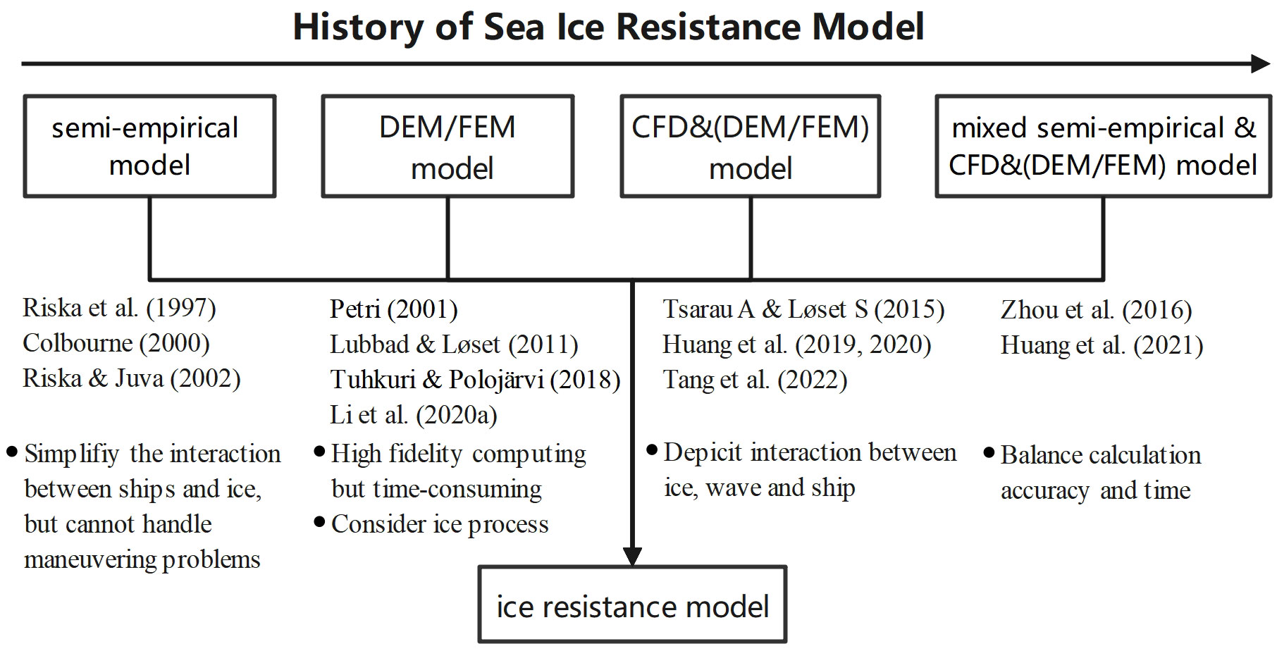
Figure 1 History of the dynamic model.

The early ice resistance model utilized a semi-empirical formula to calculate the ice resistance (Riska et al., 1997). The formula was subsequently further elaborated by (Colbourne, 2000) as follows:

$\begin{array}{ll}F{r}_p=V/\sqrt{g{h}_{i}C}& (1)\end{array}$

$\begin{array}{ll}{R}_P=0.5C_p{\rho }_{i}B{h}_i{V}^2{C}^n& (2)\end{array}$

$\begin{array}{ll}{C}_p=k_{c}F{r}_p^{-b}& (3)\end{array}$

where Fr_p denotes the ice Froude number, h_i stands for the ice thickness, C represents the ice concentration, g symbolizes the acceleration of gravity, R_p indicates the ice resistance, C_p signifies the ice force coefficient, B and ρ_i are the ship beam and the ice density, and k_c, b, and n are constants relevant to ship parameters.

These research results made important contributions to ship design and operational planning (Juva and Riska, 2002). However, semi-empirical studies cannot solve the problem of maneuvering, so it is necessary to simplify the interaction between ship and ice in order to arrive at a viable solution (Li et al., 2020b).

Thus, high-fidelity computing models based on CFD, DEM, or FEM can improve individual ice resistance (Xue et al., 2020). A mathematical model for estimating ship speed was developed, which considers the ice-breaking process (Petri, 2001). Lubbad and Løset used a closed-form solution for ice-breaking modeling to simulate the dynamic processes of the ship as it broke through the ice. The velocity of a vessel in an icy region is calculated by a numerical simulation of the ice motion (Lubbad and Løset, 2011). More complex ice processes, such as ice rotation and ice submersion, were considered in current studies (Tuhkuri and Polojärvi, 2018). Although the descriptions of the different processes were still simple and not systematically validated, they were of great importance to guide (Li et al., 2020a).

Previous simulations of ship progress through ice floes ignored the effect of hydrodynamics, which was also a key factor in ship operation in icy water (Tsarau and Løset, 2015). Huang et al. (2020) first developed a CFD and DEM approach to simulate the ship-wave-ice interactions and provide reliable resistance prediction (Huang et al., 2020). In which, standard CFD models were used for ship propulsion in open water and DEM was used to simulate the interaction between ship structures and ice floes, and fluid forces were obtained from the CFD solution to achieve ship-wave-ice coupling. The original floe-distribution algorithm was developed to import the natural ice-floe fields into the CFD & DEM model, where the floes were randomly distributed and had a range of sizes according to field measurements. The accuracy of this approach in predicting the ice-floe resistance was experimentally confirmed (Tang et al., 2022).

Although a computation method is usually affordable, the CFD and DEM model is very costly. It is impractical to run the simulation every time a resistance estimation is required. Therefore, it is necessary to develop empirical equations to quickly estimate the ice resistance (Zhou et al., 2016; Huang et al., 2021), as follows:

$\begin{array}{ll}{R}_{ice}=A\times {\rho }_i\times h\times D\times V^2\times B/L_{pp}\times C^{1.5}\times F{r}^{-0.8}& (4)\end{array}$

where A represents a coefficient dependent on ships, D denotes the ice diameter, and L_pp stands for the length between vertical lines.

So far, the dynamic method is highly accurate, and it can be utilized to simulate the variation of the load in a certain polar environment. However, due to the complicated relationship between the ice and the ocean in the polar region, there are many types of ice-strengthened vessels, and the sailing conditions are very varied. A dynamic model has to recreate all the options, and this requires a large number of computational resources. It is a small sample event with weak generalization ability, and it cannot meet the requirement of high-speed simulation in polar regions.

2.1.2 Data-driven model

The statistical models are mainly based on data driving, and the effects of sea ice and other factors on ships are investigated by statistical algorithms. For instance, the relationships between the displacement and the thickness of sea ice, the concentration of sea ice, and the ice sheet were established by regression analysis (Jeong et al., 2021).

Based on Automatic Identification System (AIS) ship data, as well as sea-ice data from satellite observations, Löptien and Axell (2014) calculated velocity using multivariate regression. The mapping relationship between the ice shelf and the ice sheet, as well as the displacement depth and direction angle, was built to predict the speed performance of the various vessels in the ice(Löptien and Axell, 2014).

As a result of the rapid development of machine learning technology, Milaković et al. (2020) applied artificial neural networks to speed up reasoning in Arctic areas. By characterizing the acceleration/deceleration effect of sea ice on the ship, the speed of the ship was calculated (Milaković et al., 2020).

The main limiting factor of data-driven speed is that sea ice data cannot be matched by ship information due to different data sources (Milaković et al., 2020). Because of the poor temporal and spatial resolution of the AIS model, it is difficult to describe the interglacial channel due to the low time and space resolution of the sea ice model. Thus, wrong velocity patterns are produced, and this influences the validity of the model training. In order to do so, Similä and Lensu (2018) utilized high-resolution Synthetic Aperture Radar images to precisely describe the polar seas. The AIS temporal and spatial data were employed to train stochastic forest models. The performance of the training was more consistent with the actual sailing speed of the vessel (Similä and Lensu, 2018).

Thus, the statistical model is to establish a general empirical relationship that can be applied to different types of ships in complex polar sea conditions. Since the model is based on ship and ice data, the results are more in line with the reality of navigation. However, because of the uncertainty and randomness in the choice of variables, the reliability and stability of the proposed model should be validated.

2.1.3 Summary

Based on the above-mentioned literature review, different types of speed inference models and their errors in predicting ship speed are sorted out in Table 1.

TABLE 1

Table 1 Summary of ship speed inference models.

In order to reduce the uncertainty of ship forecasts, improve their robustness, and save computational resources, the integration of dynamic and statistical models must be enhanced.

Figure 2 proposed a new framework where the dynamic and statistical models were combined. The framework adopted the concept of transfer learning with two stages (Zhang et al., 2022). In the first stage, the mixed dynamic models were incorporated to generate large samples of certain vessels at various operating conditions. A transfer network of ship speed in ice was constructed and pre-trained by these samples. In the second stage, it was possible to derive a quantitative relationship between environmental performance, vessel performance and velocity based on the historical navigational data through the statistical models, and thus corrected the pre-training pattern.

FIGURE 2

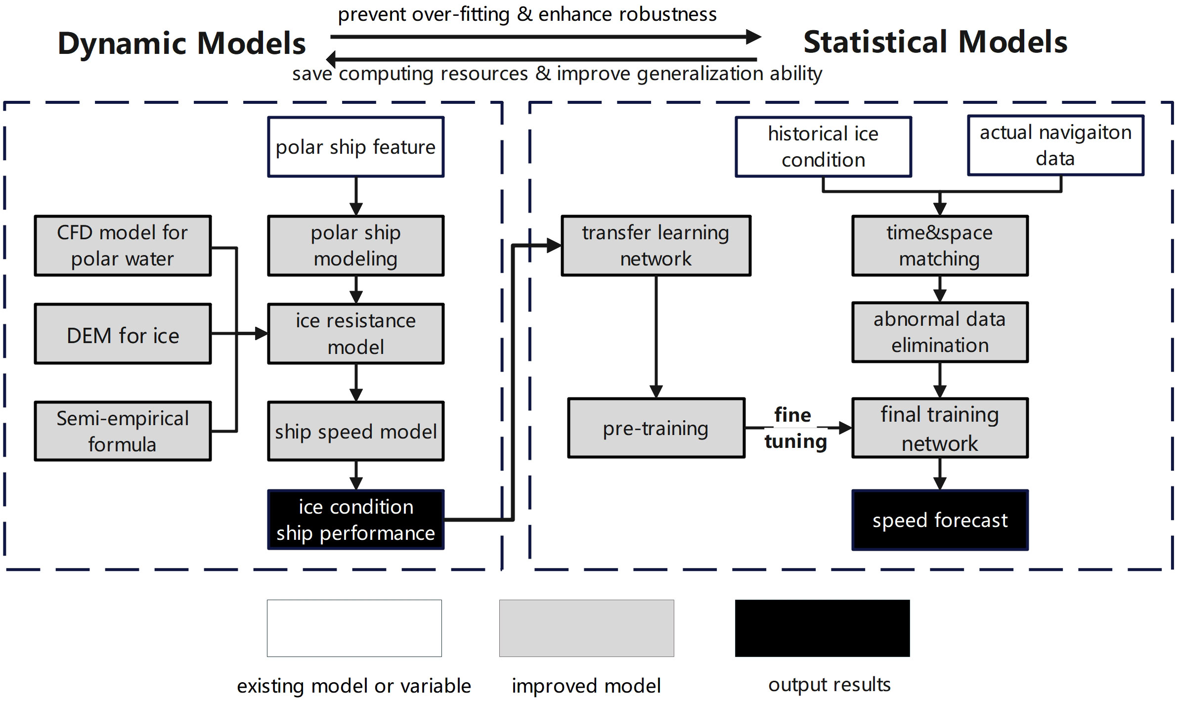
Figure 2 Speed reasoning network of coupled dynamic and statistical techniques.

2.2 Polar shipping cost

An important reason that the Arctic passage has attracted the world’s attention is the potential cost advantage of shipping due to its short distance. This is not a simple linear problem with a negative connection with the route distance.

The economic cost of navigating in the NEP depends on the ability of the ship’s ice resistance level, the cost of building the vessel, the cost of fuel (fuel consumption, fuel price, and fuel types), the operational expenses (staff wages, insurance, and repairs and maintenance), as well as the combination of several factors including piloting and ice-breaking charges (Theocharis et al., 2019). Apart from the determination of the voyage time and the area of the NEP, sea ice will also have an impact on the sailing speed, route design, and operating costs of vessels (Wang et al., 2021).

To adapt to the harsh weather and environmental conditions of the NEP, ships operating in the NEP require more powerful engines and sturdier hulls. This has resulted in higher ship-building costs compared to those of the traditional passage (Erikstad and Ehlers, 2012). As for operational costs, because of the high risk of Arctic maritime transport, extra maintenance and insurance costs have to be incurred to actively avoid accidents and mitigate risks. At the same time, crew members with ice sailing experience and the ability to cope with harsh conditions also need more salaries. Fuel cost is also one of the key factors affecting shipping costs. A ship’s fuel consumption is determined by its size, hull structure, speed, durability, and design. Since the NEP is relatively short, it is advantageous in terms of fuel expenditure. In the Arctic, however, according to the International Maritime Organization’s sulfur limit, ships have to utilize cleaner fuels at a higher cost compared to traditional fuels (Wan et al., 2018).

The estimate of the parameters in the current Arctic NEP potential evaluation models are very different and uncertain (Tables 2–4). On the one hand, the estimates of relevant factors in Arctic NEP (like ship-building, fuel, and operational costs) are highly subjective. Experts’ different understandings of the problem and optimistic and conservative expectations for the future have resulted in controversial conclusions (Theocharis et al., 2018).

TABLE 2

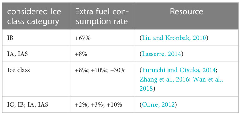
Table 2 Different conclusions regarding additional fuel costs.

TABLE 3

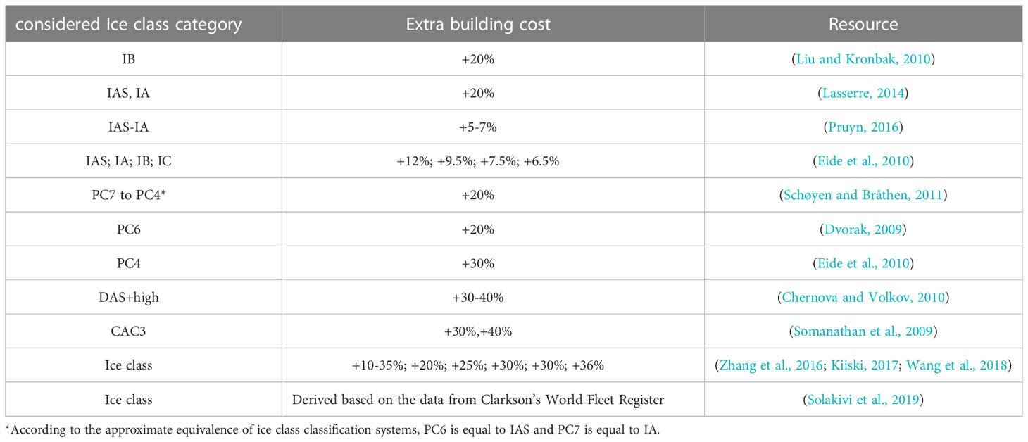
Table 3 Different conclusions regarding additional shipbuilding costs.

TABLE 4

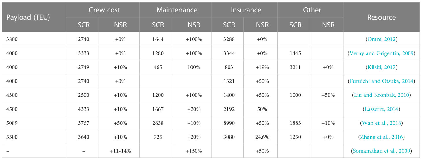
Table 4 Different conclusions regarding operating expenses (USD/day).

On the other hand, there is a lack of quantification of the multiscale effects of sea ice in the models (Wang et al., 2021). The effects of sea ice variability are usually used to determine the navigable time and navigable area. Few studies have considered the impact of sea ice changes on fuel consumption, route distance, and icebreaker charges. Models typically use many assumptions rather than parameters estimates. Although the computational complexity of the model is simplified in this way, it also brings uncertainty to the assessment. For instance, the thermal distance of the NEP is regarded as a constant, and the design of the channel does not change with changes in sea ice.

To address the aforementioned issue, Solakivi and his research team (2019) used Clarkson’s World Fleet Register data to analyze the extra economic cost of NEP vessels with various sizes/ice classes (Solakivi et al., 2019). This included extra fuel costs, extra shipping costs, and extra operational expenses. However, the data quality, the choice of factors, and the differences in statistical models have resulted in uncertainty in the outcomes of data-driven assessments. Especially, the data from the above-mentioned documents were obtained in the winter, and the samples were not sufficiently representative. Furthermore, the 2015 figures were taken into account for transportation costs up to 2022 or beyond, with no consideration for changes in the economic cost over time.

To make full use of expert knowledge and data-driven analysis, Wang et al. (2023) proposed a new framework for economic analysis of marine transportation (see Figure 3), where uncertainty is given more attention than the current research (Wang et al., 2023). First, a new quantitative method was used in conjunction with an importance ranking method to capture uncertainty in the evidence and to perform multi-source evidence fusion. Second, a Bayesian network model was chosen as a tool to convey the uncertainty from one variable to another variable. Third, the Bayesian network was well-trained by the fused multi-source evidence, and was able to combine expert knowledge and statistical results in a probabilistic manner to achieve inference about the economic costs of future polar voyages. Finally, the trained network was used for sensitivity analysis and quantitative evaluation of key factors affecting the polar economy.

FIGURE 3

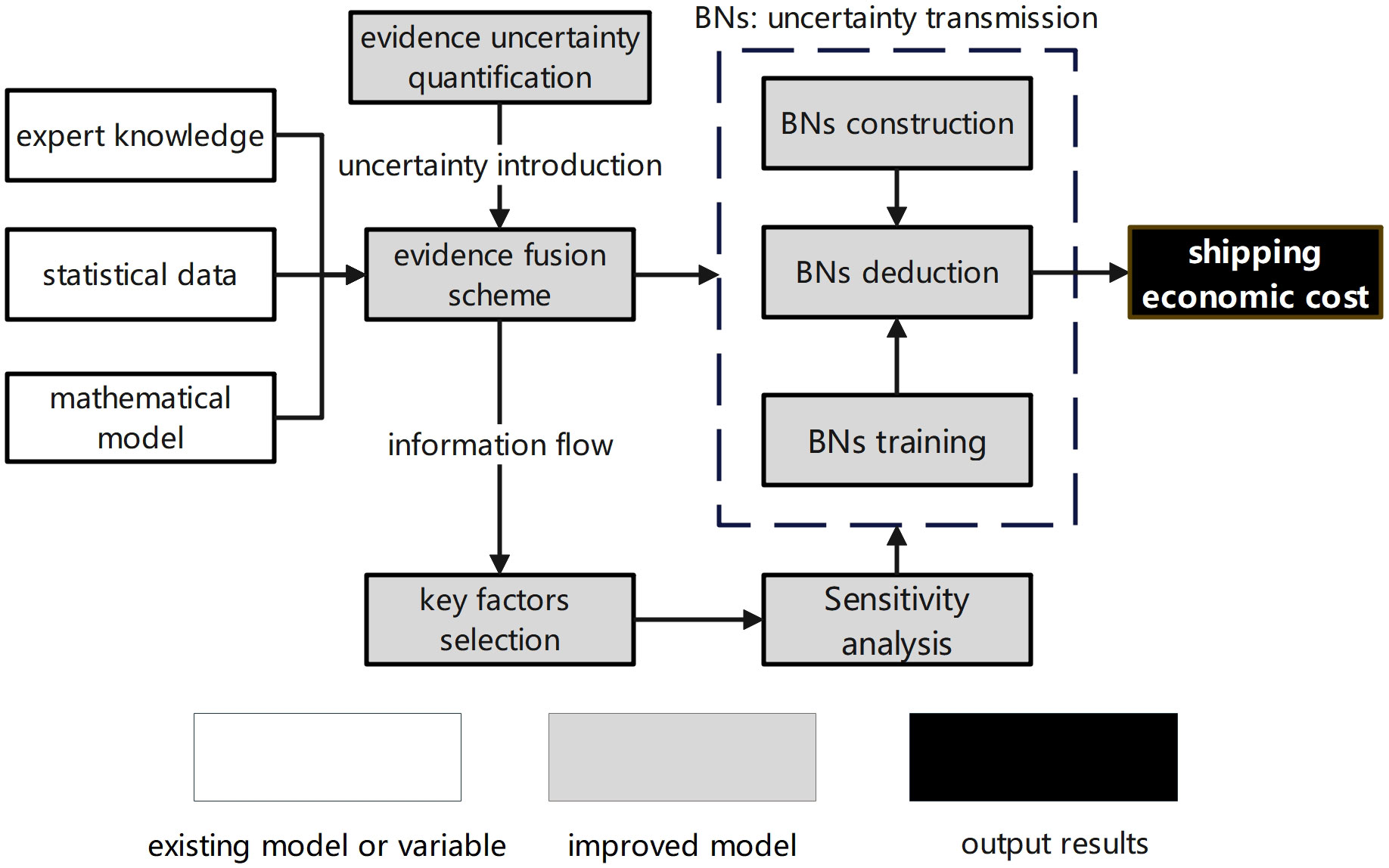
Figure 3 Multi-source heterogeneous economic cost inference model.

2.3 Polar navigation safety

For Arctic weather routing, in addition to considering the above navigation speed and navigation costs, the security of navigation is clearly of paramount importance. As a result of the unique geographical environment of the Arctic region, apart from the traditional factors such as wind, waves, and other factors, the influence of sea ice on safe navigation should be taken into account. Though the Arctic NEP is essentially navigable in the summer, there are still a few marine regions that are frozen.

There are two major types of risk evaluation in Arctic NEP. The first type is risk assessment by considering risk probability or empirical formula. The other type adopts a standardized risk quantification framework that combines critical navigation conditions (such as the sea ice index in the sea ice regional navigation system issued by Transport Canada, and the risk index in POLARIS issued by the International Maritime Organization) (Browne et al., 2022).

The benefit of risk assessment by considering risk probabilities or empirical formulas is that it is possible to draw probabilistic conclusions if the effect of sea ice is not sufficiently clear. The model of reasoning combined with the experience can provide assessment results that are consistent with general cognition. For example, Li et al. (2021b) employed the Dynamic Bayesian Network (DBN) approach to assess the navigational hazard of a particular route according to influencing factors like wind velocity, temperature, wave height, and ice depth (Li et al., 2021b). They built the network nodes according to subjective experience and computed the DBN time transmission probability. Through the dynamic time transfer nodes, the study could enable the dynamic risk assessment of probability changes as the background field changes. However, this method requires reliable expertise to determine probabilities for various types of ships, and its generality has to be reviewed. Besides, in the quantification of sea ice, the study only considered the effect of sea ice concentration, without taking into account the effect of factors like the thickness of the sea ice on the hazard and velocity of the vessel. Lehtola et al. (2019) applied a subjective experience formula to comprehensively consider the effects of sea ice concentration, thickness, and ice ridges on vessel navigation (Lehtola et al., 2019). Furthermore, the impact of sea ice on navigational risks was mapped to navigation speed for navigation. Compared with the probability of DBN, the empirical equation could provide a distinct hazard outcome. The study could also provide a reasonable quantification of factors, such as the concentration and thickness of sea ice, and the calculated results were very informative. However, the empirical formula is based on some necessary assumptions, such that calculated results are not correct and the real sailing conditions are not consistent. Moreover, the empirical formula is based on the fixed information of some factors, and it does not consider the subjective initiative of the crew in the actual voyage.

The second approach is based on determining the safe margin of navigation combined with critical navigational conditions. The POLARIS not only considers sea ice concentration and thickness data, which are the most important factors for navigation, but also takes into account seamen’s subjective experience. POLARIS integrates the related experience with other techniques, such as the Canadian Arctic Ice Navigation System, the Russian Ice Zone Certificate, and the Assistance to the Pilot Ice Zone as described in the Navigation Regulations of the Northern Sea Route (Deggim, 2018). The formula for calculating the risk value is as follows:

$\begin{array}{ll}\text{RIO}=({\text{C}}_1\times {\text{RIV}}_1)+({\text{C}}_2\times {\text{RIV}}_2)+({\text{C}}_3\times {\text{RIV}}_3)+\dots +({\text{C}}_{\text{n}}\times {\text{RIV}}_{\text{n}})& (5)\end{array}$

where C₁…C_n are the sea ice concentration, and RIV₁…RIV_n are determined by the ice level of the ship and the thickness of the sea ice (see Table 5). As a framework for navigation guidance in polar areas, the POLARIS can evaluate the navigation risks under different ice conditions according to the ice level of the ship. Based on the navigation risks, navigation instructions such as the need to slow down or to recommend detours are presented in Table 6 (Engtrø et al., 2020). The system can be utilized as a risk restraint in ship navigation, and the recommended speed is based on the risk range (Table 7). For example, Li et al. (2020b) calculated the speed of the ship through ice resistance and introduced the risk index of the POLARIS as a navigation risk constraint in route planning (Li et al., 2020b). Route planning was carried out according to the thickness and concentration of sea ice to ensure the safe navigation of ships. Lee et al. (2021) computed the sailing power based on the ship’s evaluation model and introduced the POLARIS into route planning (Lee et al., 2021). The research was based on POLARIS’ guidance to constrain the sailing speed and to ensure the safety of the planning results. For Arctic meteorological navigation, the POLARIS can not only quantify the risk of sea ice cover for ship navigation but also can regulate the navigation of ships based on the quantified risk value, which has good applicability in meteorological navigation issues.

TABLE 5

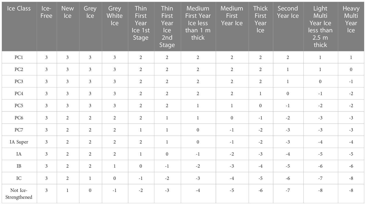
Table 5 Risk index values (Li et al., 2020b).

TABLE 6

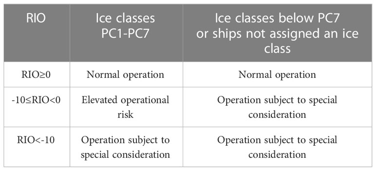
Table 6 Risk index outcome criteria (Bergström et al., 2022).

TABLE 7

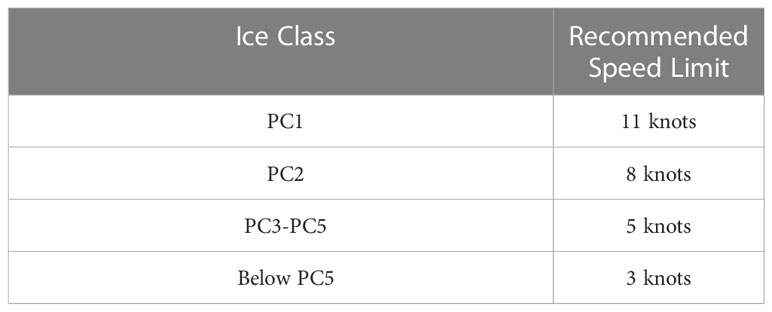
Table 7 Recommended speed limits for elevated-risk operations (Bergström et al., 2022).

3 Literature review for IRAs

The components of a route-finding algorithm can be illustrated by formulating the task in terms of an optimization problem. The objective function models the cost for a ship to travel along a given path between destination A and destination B. This cost may be measured by the journey time, the shipping costs, or the voyage risk caused by the ice loading.

3.1 Design of background field

First of all, unlike road planning, there is no fixed route in polar marine areas. The coastline map of the shipping area defines the objective functions, which can be based on various definitions, such as a grid or a diagram linking waypoints, and points in a Cartesian grid or in the form of a triangular-shaped grid (Piehl et al., 2017). Recently, several research studies have been devoted to the development of original ice routing approaches, such as the application of the Voronoi diagram (Liu et al., 2016), and the FEM-based potential theory (Piehl et al., 2017). Based on the existing research on Arctic sea route planning, the design of the background field can be divided into two categories.

One is the discrete background field, which is usually regarded as the standard grid of discretization. For example, Zhang et al. (2019) used a standard grid based on data resolution as the background field in the course simulation of multi-ship operations (Zhang et al., 2019). When Lee et al. (2021) used a genetic algorithm to plan the route in the Arctic sea, the grid of the background field is generated according to the longitude and latitude resolution of sea ice data (Lee et al., 2021). Depending on the latitude, the resolution of the grid also changes, as shown in Figure 4.

FIGURE 4

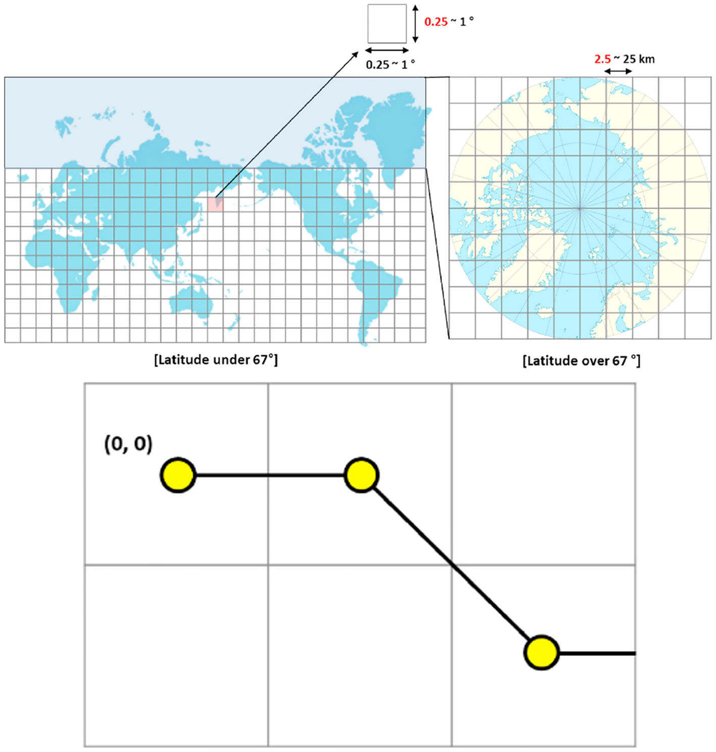
Figure 4 Background field of normalized grid points (Lee et al., 2021).

The use of discrete standard grids for background field design leads to rough routes obtained by the path planning algorithms, which need to be smoothed afterwards. Since there are only a few fixed choices of ship steering angles in a discrete background field, it is usually only possible to move from the current point to eight surrounding points (Nam et al., 2013). Some studies have interpolated sea ice elements to improve the grid resolution of the background field and reduce the roughness of the route (Kotovirta et al., 2009).

The other is the continuous background field, which is usually irregular. For example, Piehl et al. (2017) used the Delaunay triangulation method to divide the background field into fine irregular triangles, making the ship’s turning angle freer (Piehl et al., 2017). The resulting visual continuity is shown in Figure 5 below.

FIGURE 5

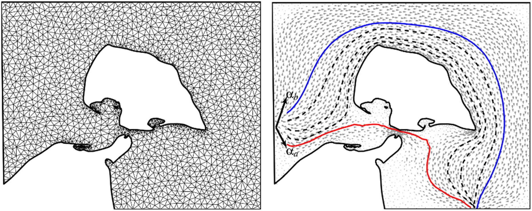
Figure 5 Background field of triangulated grid points (Piehl et al., 2017).

Similarly, Liu et al. (2016) used the Voronoi diagram method to divide the background field into irregular polygons (Liu et al., 2016). This can improve the steering freedom of the ship in the route planning algorithm and make the calculated route smoother. In addition, there are also studies on route planning based on sailing distance and turning angle, which decompose the entire route into many short routes of different lengths and angles (Lee et al., 2018). A smooth route can also be obtained by this method when the route segmentation is fine.

Although routes generated based on discrete and continuous background fields have different roughness, they often need to be smoothed at a later stage. Several studies have shown that the difference in background field design has little effect on the results of route planning, but mainly affects the calculation time of the algorithm. Despite the concern that the convergence speed in continuous conditions is usually slower in comparison to the discrete conditions because more alternatives are involved in the former, the algorithms reach an optimal solution at a similar iteration (Choi et al., 2013).

3.2 Selection of path planning algorithm

In addition to the above background field design differences, the most significant difference between ice routing studies is the choice of a path planning algorithm. In the current research on ice route planning in the Arctic, the methods used can be roughly divided into the following:

The first is a direct search algorithm, such as the Powell method. This kind of algorithm has high computational efficiency, but it is easy to fall into local optimization, and algorithm convergence is difficult (Kotovirta et al., 2009).

The second is a greedy search algorithm, such as the Dijkstra algorithm. Nam et al. applied the Dijkstra algorithm to choose the best way on a set of segments along the Northern Sea Route (Nam et al., 2013). If there is no negative objective function value in the search area, the Dijkstra algorithm can achieve the global optimal solution by checking all the explored nodes. But for a large sea area, the search speed of this algorithm will be significantly reduced, and a lot of memory will be consumed.

The third is a heuristic algorithm, such as the A* heuristic algorithm. Ice route planning based on the A* heuristic algorithm has attracted much attention in recent years because of its high search efficiency (Guinness et al., 2014). Some studies contain modifications of the basic A* algorithm for better applicability to the considered problem (Wang et al., 2018). The heuristic search algorithm can measure the distance relationship between the search location and the target location. This makes the search direction preferentially oriented to the target location and improves search efficiency.

The fourth is a random search algorithm, such as the Genetic Algorithm (GA). Choi et al. contributed to the problem of ice routing by introducing the genetic optimization algorithm instead of the “greedy” one (Choi et al., 2013). This algorithm is suitable for multi-objective programming, especially when the weight of goals cannot be measured. The random search algorithm can get a good solution quickly. But the algorithm depends on parameter initialization, and the performance of the algorithm is greatly affected by the random search operator (Katoch et al., 2021). Therefore, it is difficult for the random search algorithm to achieve global optimization.

The algorithm in the above research mainly focuses on static route planning and cannot respond to the change of background field. In addition to the above algorithms, there are also LPA* and D*lite algorithms suitable for dynamic programming. The LPA* algorithm is a forward incremental search algorithm. In a dynamic environment, the LPA* algorithm can adapt to the change of obstacles in the environment. When the obstacles change, the distance information obtained previously is used for secondary planning without recalculating the entire environment. However, this algorithm cannot guarantee the pass ability of the unsearched area, because it can only be calculated based on the distance information from the current point to the starting point and the estimated information to the target point (Koenig and Likhachev, 2005). In the process of approaching the target point, the D*lite algorithm can deal with the emergence of dynamic obstacle points through static search in the local scope. The heuristic algorithm can guide the search direction to the target point in each search, which can further improve the search efficiency by replacing the limitation of the non-heuristic algorithm to walk around without rules (Jin et al., 2023).

Considering the changes of icefloes and icebergs in the Arctic Sea, the dynamic planning algorithm is more suitable for the route in the ice region. Elements such as icefloes and icebergs usually do not have fixed drift routes, so the location or short-term prediction must be carried out based on real-time observations. Therefore, in order to deal with the variables that change with time, a dynamic path planning algorithm should be introduced to optimize routes in the Arctic Sea. The algorithm can characterize the dynamic influence of dangerous elements such as icefloes and icebergs, and adjust the route based on the constantly updated forecast data (Choi, 2015).

The present dynamic path planning algorithm can be used to describe the variation of the dynamic barrier more effectively. However, dealing with the dynamic variation of the objective function because of the variation of the sea ice is not effective. In the Arctic Sea, the dynamic changes of sea ice not only affect the points of obstacles, but also have a significant impact on the navigable grid points. As the sea ice changes at different times, the objective functions such as the risk and speed change accordingly. For instance, as the sea ice becomes thicker and thicker, the associated navigational hazards and navigational speed will be decreased and increased with time. Even though the obstacles remain unchanged, the objective function has changed with time (Wang et al., 2018). Therefore, the current dynamic path planning algorithm has application problems in Arctic Weather Routing, which need to be further studied and improved.

3.3 Diversity of objective functions

Because of the special nature and ecology of the Arctic region, the route planning for the Arctic Sea should not only consider the changes in the environmental field, but also consider a variety of constraints. As far as the restriction is concerned, the terrain restriction is static and depends on the vessel’s type and relative parameters (e.g., dimension, shape, and draft). In the future, the dynamic variation of sea ice is a critical factor that will limit the opening of NEP. (Zhang et al., 2017) presented a new approach to scheduling Arctic maritime routes with multiple constraints on physical and operational aspects.

As for the object function, the primary aim of Arctic Route Planning is to guarantee safe sailing and prevent damage to the ship due to the harsh environmental conditions. (Li et al., 2021b) adopted DBN to build a road safety assessment model based on environmental factors such as sea ice, which could be utilized to dynamically evaluate the voyage hazard. In addition to security, the cost of navigation should also be taken into consideration. (Topaj et al., 2019) utilized economical criteria to optimize the route design and to make sure that the target can be reached within the scheduled time. At the same time, they not only saved the cost of fuel and other costs but also avoided the problem of damages for violation of the contract due to excessive sailing time. Furthermore, the timeliness of navigation is also crucial. A number of studies have considered polar climates and have employed voyage time as an objective function when planning a path to minimize fuel consumption and to make sure that the destination port is reached on time (Kuhlemann and Tierney, 2020).

Based on the above-complicated constraints and objective functions, it is clear that the single-objective path planning algorithm has no capability. Thus, it is necessary to adopt multi-objective route planning. The existing research on multi-objective processing is mainly divided into two methods:

One is to introduce subjective knowledge optimization methods, such as the weighting method, constraint method, and linear programming method. Based on the theory of weights, constraints, and linear programming, a multi-objective function can be converted into a single-objective function. The multi-objective function is solved by the single-objective optimization method. Although this method makes the solution less difficult, it is possible to obtain only one solution, like (Lehtola et al., 2020) who implemented the auto-route optimization with the A * algorithm. Taking into account the timeliness and security characteristics of vessels operating in the Arctic NEP, this optimal framework was developed to assign different weights. In the actual decision-making process, the distribution of weighted values is more subjective. Conflicts may exist between objectives, and it is difficult to specify accurate weights to optimize them all at once.

The other one is based on Pareto optimal solution. This method can find a set of solutions that make each target value compromise, that is, the Pareto optimal solution, to provide a variety of alternative solutions according to different needs. For example, Zhang et al. (2021) used the improved ant colony evolution algorithm to build different types of multi-objective route planning models, aiming at route optimization among conflicting objectives (sailing time, additional navigation resistance, and navigation safety) (Zhang et al., 2021). Fabbri and Vicen-Bueno (2019) introduced the second-generation fast non-dominated genetic algorithm (NSGA-II) to solve the Pareto optimal set under multi-objective conditions (Fabbri and Vicen-Bueno, 2019).

However, the application of the multi-objective optimization method in the Arctic Sea is less. Considering that the multiple objective functions to be considered in the Arctic route planning are complicated, it is difficult to give weights based on subjective knowledge. Therefore, multi-objective optimization algorithms based on Pareto have high applicability, such as the NSGA-II algorithm. More research should be done on multi-objective optimization in Arctic Weather Routing.

4 Discussion

Since most of the research on IRAs in Section 3.2 used only one algorithm, the differences between algorithms were not compared. Therefore, we replicated and compared the existing algorithms with experiments based on the background field of normalized grid points to study the effects of different algorithms under different objective functions. In addition to the static path planning algorithm in Section 3.2, we also introduced the D*lite dynamic path planning algorithm here. The applicability of static and dynamic path planning algorithms in ice route planning was tested.

Further, through the literature review in Section 3, we identified the problem in the current research, i.e., how to deal with the dynamic multi-objective path planning in the Arctic Sea. There would be a variety of solutions to this problem, and we proposed a solution here, the D*-NSGA-III algorithm. We compared the dynamic multi-objective optimization capability of D*-NSGA-III algorithm based on the replication and comparison experiments of existing algorithms.

4.1 Data description

This experiment used the sea ice thickness data of PIOMAS (Pan-Arctic Ice-Ocean Modeling and Assimilation System) and the sea ice concentration data of NSIDC (National Snow and Ice Data Center). The spatial resolution was unified to a grid of 0.25°×0.25°, and the time resolution was one day. The ship navigation data of the IA ice class was derived from Automatic Identification System (AIS).

Sea ice concentration from the National Snow and Ice Data Center (NSIDC) is a daily grid data. The data was synthesized from the Nimbus-7 satellite and microwave detection data from the Defense Meteorological Satellite Program (DMSP) and DMSP-F17 satellite (Tschudi et al., 2020).

PIOMAS is an Arctic sea ice numerical simulation system that includes multiple elements of sea ice and ocean (Zhang and Rothrock, 2003). Improving numerical simulation results by assimilating sea surface temperatures from ice-free areas and using different ice strength parameters can provide daily grid data on sea ice thickness.

AIS is a modern navigational aid system that transmits information such as ship speed back to ground base stations. The frequency reported by the ship is generally 12 seconds/time, and when the course changes, it is generally 4 seconds/time. The AIS data set of 2018 was used in this experiment. The ice class of the ship was Class IA and the speed was up to 22 knots.

4.2 Design of experiment

This experiment is divided into two main parts. The first part of the experiment, based on four algorithms (D*lite, A*, Dijkstra, GA), takes navigation safety cost (RIO), sailing time cost (Time), and sailing distance cost (Distance) as a single objective function to test the effectiveness of the four algorithms.

In the second part of the experiment, the D*-NSGA-III algorithm is used to obtain the Pareto optimal solution set of the dynamic multi-objective path planning problem by considering the constraints of three objective functions, RIO, Time, and Distance, under the dynamic background field. By comparing with the results of the first part, we test whether the algorithm can be used to solve the dynamic multi-objective path planning problem in the Arctic Sea, and verify the effectiveness of the algorithm.

To control the variables, the following experiment takes the port of Petropavlovsk-Kamchatskiy (53°1′N,158°39′E) as the start point and the port of Rotterdam (51°55’ N, 4°29’E) as the endpoint. This experiment assumes November 2, 2020, as the departure time, and only two environmental factors, sea ice concentration and sea ice thickness, are considered. Navigation risk is calculated based on the RIO value of the POLARIS. The speed inference model is based on the random forest algorithm to fit the relationship between sea ice concentration, thickness and ship speed (Wang et al., 2021). The area where RIO is less than -10 is considered as an unnavigable obstacle. The area of RIO between -10 and 0 is considered to require icebreaker assistance, and the speed is fixed at 4 knots. The area of RIO between 0 and 30 is calculated by the random forest model. Areas of RIO greater than or equal to 30 are at full speed, with a speed of 22 knots.

In the first part of the experiment, only two variables of the algorithm (4 kinds) and the objective function (3 kinds) are changed in this study, and a total of 12 route planning results are obtained. Three aspects of work have been carried out:

Firstly, the effects of algorithms on ice route planning (taking A*, Dijkstra, GA as examples) are compared.

Secondly, the influence of different objective functions on the route planning algorithm is verified.

Thirdly, the applicability of static path planning algorithm and dynamic path planning algorithm (taking D*lite as an example) in ice route planning is tested.

In the second part of the experiment, this study uses the D*-NSGA-III algorithm to obtain the Pareto optimal solution set by taking RIO, Time, and Distance as multi-objective constraints. To clearly show the result of path planning, this paper only shows three optimal paths under different goals.

4.3 D*-NSGA-III

Because the D*lite algorithm only updates the values of adjacent or related points when the obstacle is changed. The remaining grid points which are always passable still retain historical values. Therefore, the objective function value of the passable point does not change with the background field, resulting in the feasible solution found by the algorithm not being the optimal solution.

In addition, D* lite has a problem with addressing multiple objectives during the planning. This algorithm takes the utility function as the basis of the choice of the route. Although the multi-pole utility function can be set at the same time, there is still a need to enhance the consistency and understanding of the various objectives. The NSGA algorithm performs well in multi-objective optimization. Furthermore, NSGA-III improves the crowding classification of population screening more than NSGA-III, thus allowing more diversity of algorithm results (Deb and Jain, 2014). The NSGA-III algorithm is employed to randomly find the best solution in the solution space, and it is utilized to generate a new population. The algorithm is based on the Pareto theory and uses non-dominant sorting to sort and filter the crossed and mutated populations. The diversity of the screened populations is guaranteed through preset reference points. However, NSGA-III also has some problems with Arctic weather navigation. The population initialization is complicated, particularly in the Arctic meteorological navigation, and it is difficult to find a viable solution to accommodate the variations in the background field.

In summary, the optimization of the Arctic NEP should not only deal with the dynamic variation of the parameters and the utility function but also should deal with the multi-objective function constraints. To solve this dynamic multi-objective ice routing planning problem, we propose a possible solution. Based on the population iterative optimization framework of NSGA-III, we combine D*lite and NSGA-III algorithms to propose D*-NSGA-III algorithm. The technical flow of the algorithm is shown in Figure 6 below.

FIGURE 6

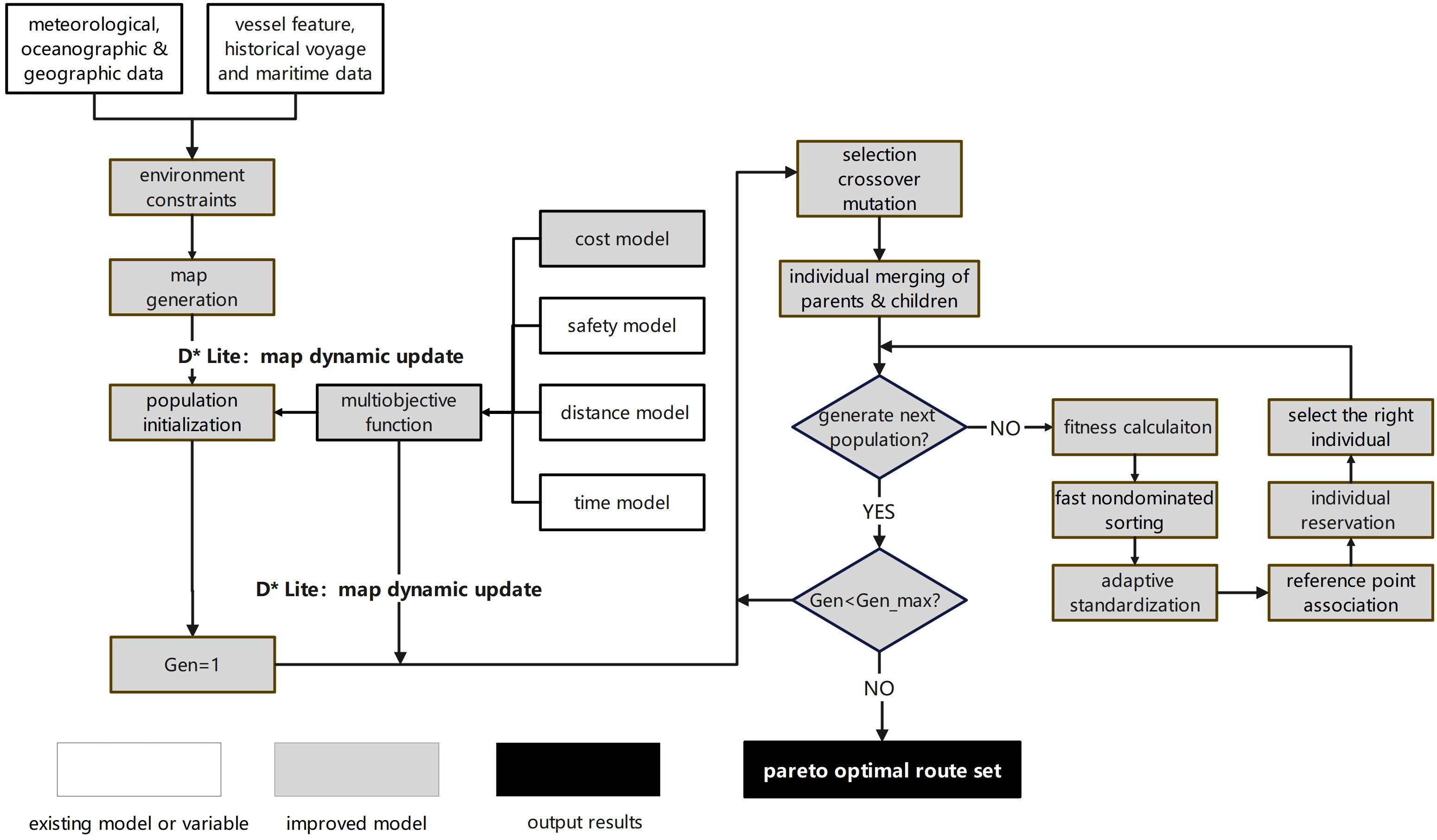
Figure 6 D*-NSGA-III dynamic multi-objective path planning model.

In the initialization module, the D*lite algorithm can smoothly generate the initial population, even though it is not necessarily the best estimate. Based on the population generated by D*lite initialization, NSGA-III can find the Pareto optimum through cross-variation and population selection. Ultimately, the D*-NSGA-III algorithm can come up with multiple sets of feasible solutions. The solution distributed on the leading edge of Pareto is the optimal solution under the multi-objective function constraints, and the appropriate route can be chosen based on the different navigation tasks.

4.4 Objective function

In this experiment, the calculation of safety cost is based on the RIO value in Section 2.3. The value of RIO in POLARIS ranges from -10 to 30. A larger value indicates more security. The safety cost of navigation adopts the cumulative RIO value method:

$\begin{array}{ll}S={\displaystyle \sum _i(40-(RI{O}_i+10))}& (6)\end{array}$

Where i represents the grid point through which the route passes. Since the cost function in the algorithm should be as low as possible, we invert RIO when calculating the cumulative value of the cost function and adjust it to the range of 0~40.

The cost of route distance D is calculated based on the results of track planning as follows:

$\begin{array}{ll}D={\displaystyle \sum _i{D}_i}={\displaystyle \sum _{i}R\times \text{arcos}[\text{cos(}{y}_{\mathit{1}i}\text{)cos(}{y}_{\mathit{2}i}\text{)cos(}{x}_{\mathit{1}i}-x_{\mathit{2}i}\text{)+sin(}{y}_{\mathit{1}i}\text{)sin(}{y}_{\mathit{2}i})]}& (7)\end{array}$

where R is the radius of the earth, and (x_li,y_li), (x_2i,y_2i) are the latitude and longitude of the two points i in the segment. The distance is measured in nautical miles (nm).

The cost of sailing time T is calculated based on the distance and the average speed of the two points, as follows:

$\begin{array}{ll}T={\displaystyle \sum _i{D}_i/(V_{1i}+V_{2i})}& (8)\end{array}$

Where D_i is the sailing distance between two points, V_1i and V_2i are the speed at two points of the course. The speed is obtained by the speed inference model established in Section 4.2. Sailing time is measured in hours.

4.5 Replication and comparison of existing studies

For the static planning algorithm (A*, Dijkstra, GA), since the algorithm could not consider the daily refresh of the background field, the sea ice concentration and thickness on November 2 are always used as the background field for navigation planning. The population number of the GA algorithm is 100 and the number of iterations is 300. As for the dynamic planning algorithm (D*lite), the algorithm can update the sea ice background field every day, and continue to plan the subsequent route according to the changes in obstacles.

The above four algorithms are executed three times and set as the objective functions of RIO, Time and Distance, respectively. Finally, 12 routes are obtained for comparison.

The navigability and objective function values of the above 12 routes are calculated under the actual dynamic navigation environment. From November 2, when the sailing time of the route accumulates for one day, the background field is refreshed to the sea ice value of the next day. The navigability and objective function values of each route are shown in Table 8 below.

TABLE 8

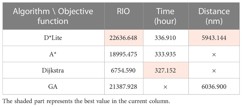
Table 8 The navigability and single-objective function value of 12 routes (× represents that the route is actually impassable).

The orange marks in Table 8 are the optimal results for the corresponding single-objective function. As can be seen from the table, when RIO is taken as the objective function, that is, the pursuit of the lowest cost of navigation safety, all routes of the 4 algorithms can be used, and the D*Lite algorithm has the best results. Among the static planning algorithms (A*, Dijkstra, GA), GA has the best effect.

However, taking the shortest time or shortest distance as the single-objective function will cause some statistical routes to be impassable. Because the routes with a short time or short distance tend to the high-latitude sea areas. However, most of the high-latitude sea areas are covered by sea ice and the sea ice changes significantly. Most of the existing studies on ice route planning are static algorithms, which can only consider a constant background field. However, when the high-latitude sea ice changes day by day, the sea ice in some areas may become thicker, resulting in some points in the static route being impassable.

All navigable routes are shown in Figure 7 below.

FIGURE 7

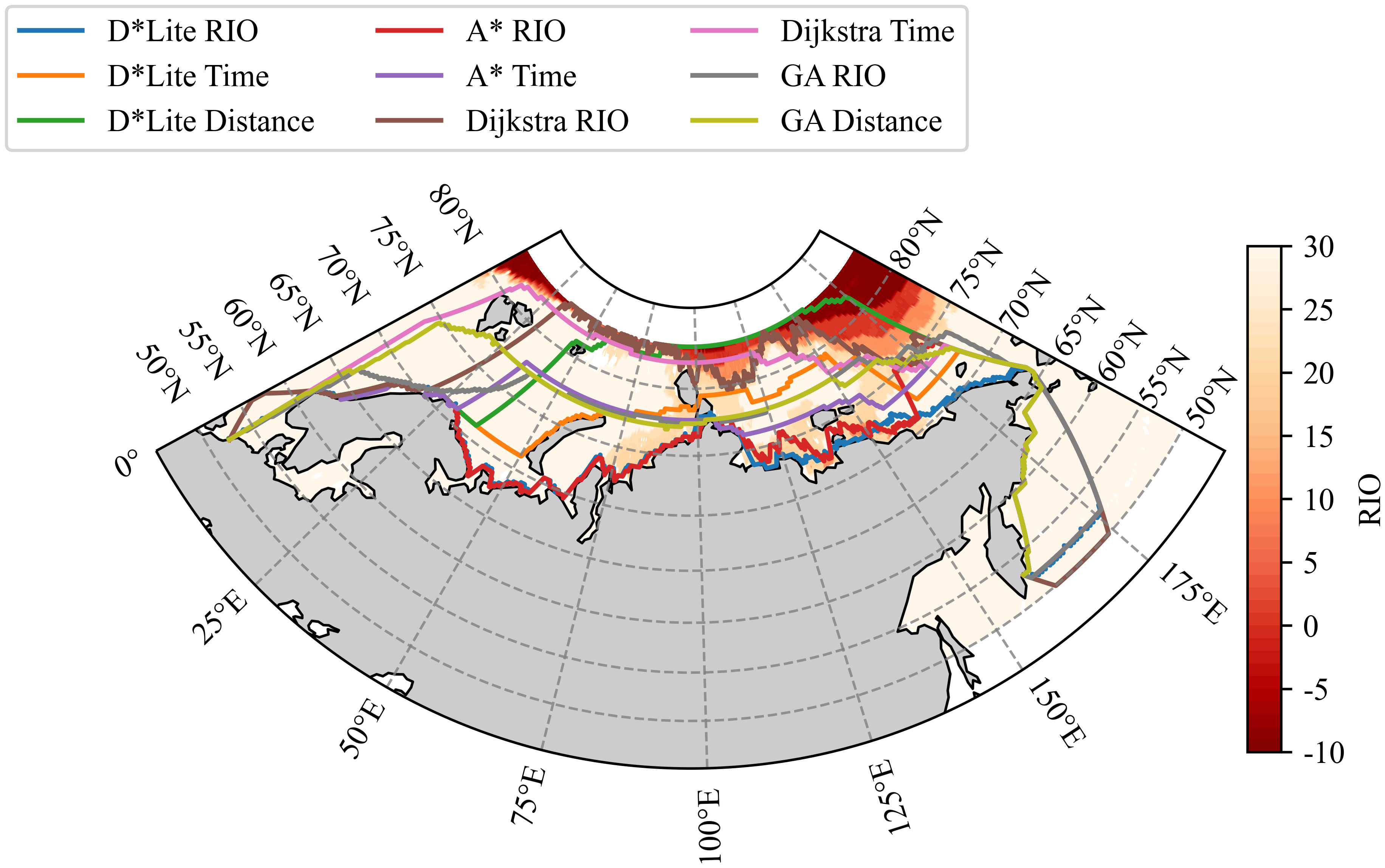
Figure 7 Passable route of path planning algorithm. The lines with different colors represent the route planning results of different algorithms (A*, Dijkstra, GA, D*Lite) under different single objective functions (RIO, Time, Distance).

From the above figure, there are obvious differences in the route planning results of the same algorithm with different objective functions. Routes with lower navigation safety costs are mostly located in low-latitude sea areas, while routes with lower time cost and lower distance cost tend to be in high-latitude sea areas. To better reflect the relationship between dynamic changes of background field and route planning, we show the route planning process with RIO, SIC, and SIT as background in (Appendix Figures 10-12) .

The data resolution used in this experiment is 0.25°, which is undoubtedly rough for product applications. It can be seen from the experimental results that the rough resolution will lead to the obvious sawtooth of the route, as shown in Figure 6. However, the purpose of this experiment is to compare the applicability of different IRAs in the Arctic. A resolution of 0.25° or finer may affect the results of the algorithm, but it should not materially affect them.

In general, the existing research on ice route planning mostly uses static planning algorithms, and there are some cases of unnavigable routes in the actual dynamic background field of ice navigation. The dynamic path planning algorithm, such as D*Lite, can be applied to the dynamic changes of Arctic sea ice and has a good application prospect. However, D*Lite cannot refresh the objective function values of globally passable grid points, and its applicability needs to be further improved.

In addition, different objective functions will have different effects on the path planning results. The Arctic Weather Routing involves a variety of objective functions, so how to reasonably carry out multi-objective route planning is also an important research direction in the future.

4.6 Effectiveness of D* -NSGA-III

From November 2, 2020, the sea ice background field was updated daily along with the accumulation of time. The population size of the D*-NSGA-III model was set to 300. The initial population was generated by the D*Lite module based on different objective functions, and the path individuals were repeated to 300 to ensure that the individuals of the initial population were passable. In the course of crossing, two intersections of different routes were selected randomly to cross and swap paths in this section. The mutation node was randomly selected during mutation. After the node’s position was changed, if a continuous route could still be found, the mutation would be considered successful. After 100 iterations, the effect of the model tended to be stable, and the individuals in the final population were all F1 individuals, that is, the Pareto optimal solution set. The Pareto surface formed by this solution set was shown in Figure 8 below:

FIGURE 8

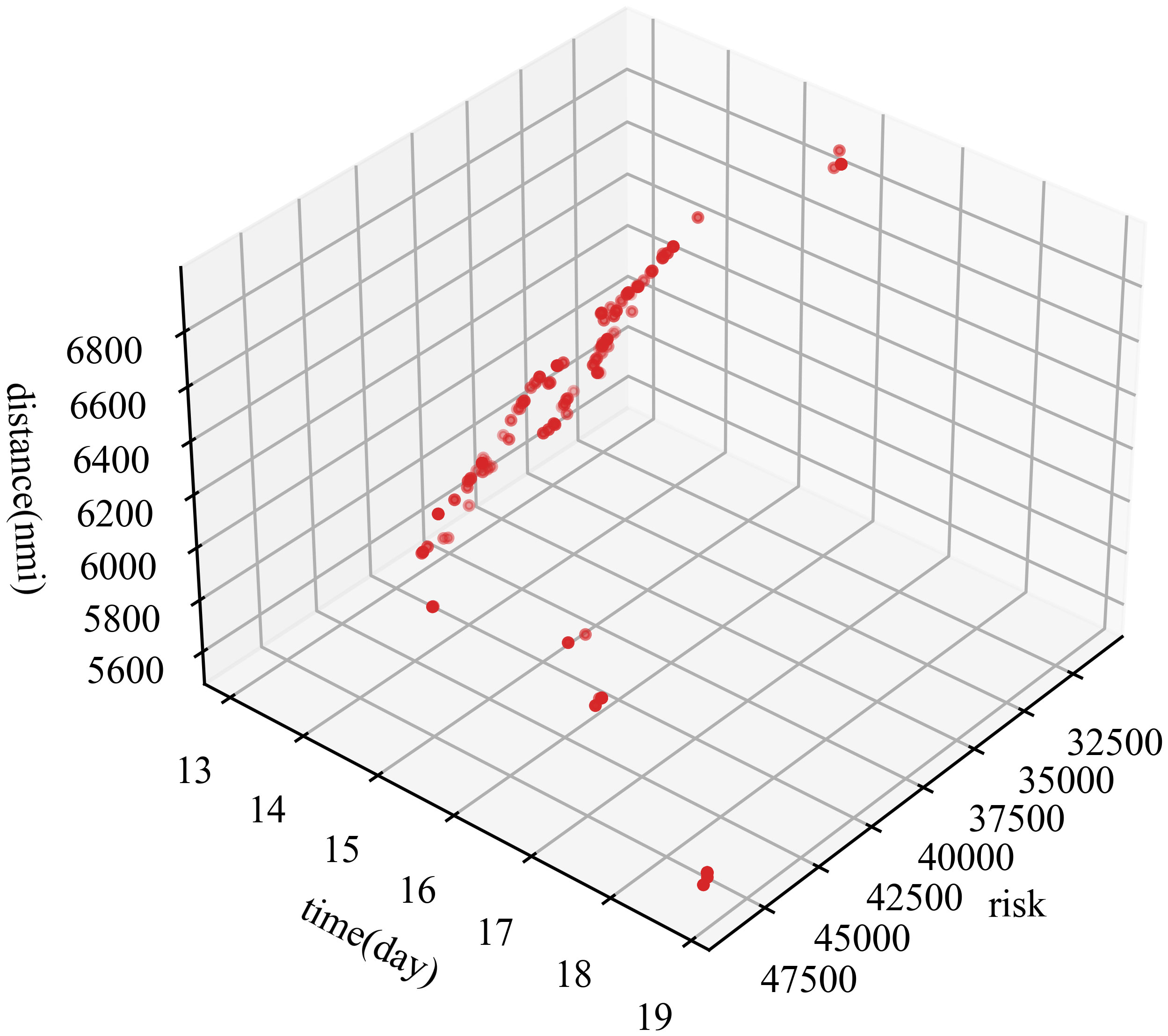
Figure 8 Distribution of optimal solution set of D*-NSGA-III. The points represent the fitness of the objective function for each path. Since all individuals are F1 individuals, the same color is used.

From the above graph, it can be observed that the optimal results of D*-NSGA-III have excellent population diversity. To pursue the shortest voyage, the lowest voyage risk, and the shortest voyage time, or to seek a compromise between several objectives, the Pareto surface, which consists of the above-mentioned points, may serve as a base for selecting routes.

Since there are multiple routes on the Pareto surface, to clearly show the route planning process and facilitate comparison with Tables 8, 9 only shows the three optimal individuals (Individual 1~3) in the optimal order of RIO, Time and Distance, respectively. Taking Individual 1 as an example, this individual has the lowest risk (the highest RIO) in the Pareto surface, as well as the best time and distance costs. Similarly, Individual 2 has the shortest time cost and Individual 3 has the shortest distance cost. The specific values are shown in Table 9.

TABLE 9

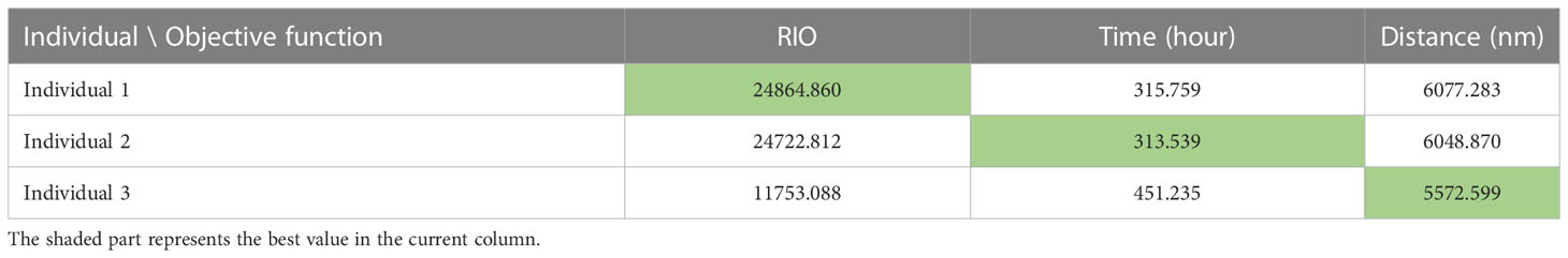
Table 9 Multiple objective function values of 3 routes.

The green marks in Table 9 represent the individual results with the optimal objective value in the Pareto solution set when single-objective sorting (columns in the table). Because D*-NSGA-III is a multi-objective optimization algorithm, all individuals (rows in the table) have three target values. By comparison with Table 8, it can be seen that when only pursuing a certain objective is optimal, the result of D*-NSGA-III is superior to the other four algorithms. In addition, D* -NSGA-III can consider a variety of objectives, so that the other two objectives are also relatively optimal.

The dynamic process of the above three routes over time is shown in Figure 9 below, taking the RIO background field as an example:

FIGURE 9

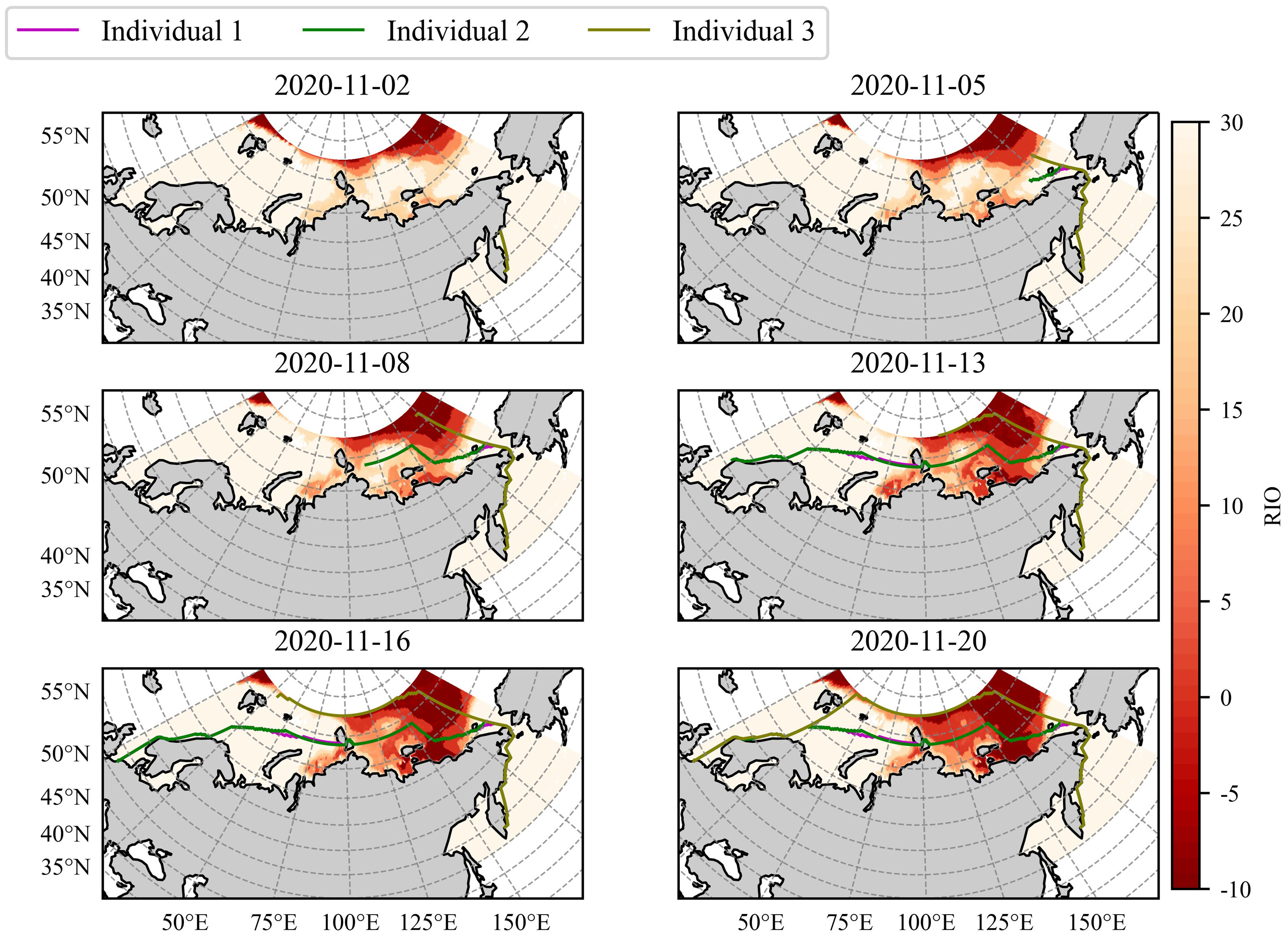
Figure 9 Individual 1~3 dynamic multi-objective route planning results. Individual 1 and 2 overlap for the most part.

As can be seen from Figure 9, D*-NSGA-III can provide the optimal route with multi-objective optimization according to different mission objectives. When in pursuit of the lowest risk of navigation (Individual 1) or the shortest voyage time (Individual 2), the two routes have high consistency, that is the mid-ocean route. It can not only avoid the time cost caused by long distances in low-latitude sea, but also avoid the time cost caused by high risks in high-latitude sea. When pursuing the shortest sailing distance (Individual 3), the route will be biased towards the high-latitude sea. At the same time, it can ensure the navigability of the route and the relatively optimal navigation risk and navigation time. In order to clearly show the route planning process, only 3 routes are shown here. The appendix shows the route planning process of all Pareto optimal solutions (Appendix Figures 13-15).

Based on the experiments, the D*-NSGA-III algorithm can satisfy the requirement of designing multi-target routing in Arctic waters. D*-NSGA-III can be employed as a guide for multi-target navigation missions.

5 Conclusion

Our research team has been working on the development of two key components of e-navigation, namely the ship performance methods and ice routing algorithms. The validity of these two models was assessed separately, the shortcoming of existing research was pointed out, and further development of this model was also discussed. Based on the replication and comparison of experiments, we examined the existing research on ice routing planning and pointed out the application prospects of dynamic routing algorithms. This paper proposed a solution to the dynamic multi-objective planning problem in Arctic waters (D*-NSGA-III) and pointed out the future research directions for Arctic weather routes.

● Based on the concept of transfer learning, the combination of dynamic and statistical models contributes to improve the robustness and generalizability of velocity forecasting.

● Leveraging expertise and statistics, and combining expertise with statistics in a probabilistic manner, enables the justification of the economic cost of polar navigation based on multi-source heterogeneous evidence.

● Forecasts based on sea ice concentration and sea ice thickness allow the estimation of navigational hazards under critical navigational conditions, making quantitative results more realistic.

● Dynamic route planning algorithm based on multi-objective optimization has a good application prospect in Arctic Weather Routing.

According to the review and analysis of IRAs, the present IRAs are not appropriate for the multi-scale dynamic variation in the Arctic NEP. Moreover, it is impossible to guarantee the diversity of the Pareto optimal solution set. Given these deficiencies, we presented a new adaptation of the IRA, named D*-NSGA-III. The validity of this algorithm was demonstrated by an example. It was proved that the proposed algorithm can achieve multi-objective optimization in the case of sea ice variation, which could satisfy the various requirements of marine transport.

However, because of the limitations of the current measurement techniques, large-scale measurements of sea ice concentration and thickness are mostly based on satellite inversion. There is still room for improvement in the accuracy of the satellite observation data, but the most significant issue is the resolution of the observed data. Different elements of sea ice often need to be observed from a distance. Besides, technical restrictions make it challenging to have accurate observations across the Arctic. Moreover, there is a spatial discontinuity in the background field data from various sources. Some of the background fields are thick, while others are thin. Therefore, it is necessary to deal with the placement and fusion of different grids. Currently, the available resolution of sea-ice data (e.g., ERA5 reanalysis datasets) is usually 0.25° x 0.25°, which is unsuitable for weather navigation (Bormann et al., 2013). Though the SAR satellite has a high resolution, it is impossible to ensure continuous observation, and it is possible to observe only a tiny portion of the ocean.

In the future, the Arctic weather routing should nest grids of different resolutions based on background fields of different spatial resolutions to realize multiscale path planning. It is possible to employ the background field of the numerical model and build the background area of the route planning through multiple grid nets. Multigrid nesting has been applied in the weather model, where a coarse grid indicates the global situation and the nesting of one or more sub-regions (Krol et al., 2005). Likewise, when the background field of route planning is built, the edge region can be procured using thicker resolution data. A delicate mesh is embedded when the marine region or certain vessel region is highly resolved. Thus, it is possible to unify the data of different resolutions to construct a background field for multiscale planning.

Data availability statement

Publicly available datasets were analyzed in this study. This data can be found here: http://psc.apl.uw.edu/research/projects/arctic-sea-ice-volume-anomaly/data/model_grid https://nsidc.org/data/G02202/versions/4.

Author contributions

QL: methodology, algorithm implementation, literature collation. YW: methodology, writing- original draft preparation. RZ: supervision, conceptualization, language editing. HY: data curation, validation. JX: language editing.YG: literature collation. All authors contributed to the article and approved the submitted version.

Funding

The author(s) disclosed receipt of the following financial support for the research, authorship, and/or publication of this article: This work has received funding from the Chinese National Natural Science Fund (No. 41976188) and the Natural Science Foundation of Hunan Province of China (No. 2021JJ40669).

Conflict of interest

The authors declare that the research was conducted in the absence of any commercial or financial relationships that could be construed as a potential conflict of interest.

Publisher’s note

All claims expressed in this article are solely those of the authors and do not necessarily represent those of their affiliated organizations, or those of the publisher, the editors and the reviewers. Any product that may be evaluated in this article, or claim that may be made by its manufacturer, is not guaranteed or endorsed by the publisher.

Supplementary material

The Supplementary Material for this article can be found online at: https://www.frontiersin.org/articles/10.3389/fmars.2023.1190164/full#supplementary-material

References

Agarwal R., Ergun Ö. (2008). Ship scheduling and network design for cargo routing in liner shipping. Transp. Sci. 42, 175–196. doi: 10.1287/trsc.1070.0205

CrossRef Full Text | Google Scholar

Bergström M., Li F., Suominen M., Kujala P. (2022). A goal-based approach for selecting a ship’s polar class. Mar. Struct. 81, 103123. doi: 10.1016/j.marstruc.2021.103123

CrossRef Full Text | Google Scholar

Bormann N., Fouilloux A., Bell W. (2013). Evaluation and assimilation of ATMS data in the ECMWF system. J. Geophys. Res. Atmospheres 118, 12,970–12,980. doi: 10.1002/2013JD020325

CrossRef Full Text | Google Scholar

Browne T., Tran T. T., Veitch B., Smith D., Khan F., Taylor R. (2022). A method for evaluating operational implications of regulatory constraints on Arctic shipping. Mar. Policy 135, 104839. doi: 10.1016/j.marpol.2021.104839

CrossRef Full Text | Google Scholar

Chen J., Kang S., Chen C., You Q., Du W., Xu M., et al. (2020). Changes in sea ice and future accessibility along the Arctic Northeast Passage. Glob. Planet. Change 195, 103319. doi: 10.1016/j.gloplacha.2020.103319

CrossRef Full Text | Google Scholar

Chernova S., Volkov A. (2010). Economic feasibility of the Northern Sea Route container shipping development. Master’s thesis. Norway: Bodø University College. 124.

Google Scholar

Choi M. (2015). Arctic sea route path planning based on an uncertain ice prediction model. Cold Reg. Sci. Technol. 109, 61–69. doi: 10.1016/j.coldregions.2014.10.001

CrossRef Full Text | Google Scholar

Choi M., Chung H., Yamaguchi H., De Silva L. W. A (2013). Application of Genetic Algorithm to Ship Route Optimization in Ice Navigation. in Proceedings of the International Conference on Port and Ocean Engineering Under Arctic Conditions (Espoo, Finland).

Google Scholar

Colbourne D. B. (2000). Scaling pack ice and iceberg loads on moored ship shapes. Ocean. Eng. Int. 4 (1), 39–45.

Google Scholar

Deb K., Jain H. (2014). An evolutionary many-objective optimization algorithm using reference-point-based nondominated sorting approach, part I: solving problems with box constraints. IEEE Trans. Evol. Comput. 18, 577–601. doi: 10.1109/TEVC.2013.2281535

CrossRef Full Text | Google Scholar

Deggim H. (2018).“The International Code for Ships Operating in Polar Waters (Polar Code),” in Sustainable Shipping in a Changing Arctic WMU Studies in Maritime Affairs. eds. Hildebrand L P., Brigham L. W., Johansson T. M. (Cham: Springer International Publishing), 15–35. doi: 10.1007/978-3-319-78425-0_2

CrossRef Full Text | Google Scholar

Dvorak R. E. (2009). Engineering and economic implications of ice-classed containerships. Thesis. Cambridge, MA: Massachusetts Institute of Technology, 93.

Google Scholar

Eide L. I., Eide A., Endresen Ø. (2010). Shipping across the Arctic Ocean: A feasible option in 2030-2050 as a result of global warming. Research and Innovation Position Paper 04-2010. 2010. Available at: https://www.yumpu.com/en/document/ view/10675657/shipping-across-the-arctic-ocean-positionpaper-dnv.

Google Scholar

Engtrø E., Gudmestad O. T., Njå O. (2020). The polar code’s implications for safe ship operations in the arctic region. TransNav 14, 655–661. doi: 10.12716/1001.14.03.18

CrossRef Full Text | Google Scholar

Erikstad S. O., Ehlers S. (2012). Decision support framework for exploiting northern sea route transport opportunities. Ship Technol. Res. 59, 34–42. doi: 10.1179/str.2012.59.2.003

CrossRef Full Text | Google Scholar

Fabbri T., Vicen-Bueno R. (2019). Weather-routing system based on METOC navigation risk assessment. J. Mar. Sci. Eng. 7, 127. doi: 10.3390/jmse7050127

CrossRef Full Text | Google Scholar

Furuichi M., Otsuka N. (2014). Economic feasibility of finished vehicle and container transport by NSR/SCR-combined shipping between East Asia and Northwest Europe. in International Association of Maritime Economists Conference 2014 (Norfolk, USA).

Google Scholar

Guemas V., Blanchard-Wrigglesworth E., Chevallier M., Day J. J., Déqué M., Doblas-Reyes F. J., et al. (2016). A review on Arctic sea-ice predictability and prediction on seasonal to decadal time-scales. Q. J. R. Meteorol. Soc 142, 546–561. doi: 10.1002/qj.2401

CrossRef Full Text | Google Scholar

Guinness R. E., Saarimaki J., Ruotsalainen L., Kuusniemi H., Goerlandt F., Montewka J., et al. (2014). “A method for ice-aware maritime route optimization,” in 2014 IEEE/ION Position, Location and Navigation Symposium - PLANS 2014 (Monterey, CA, USA: IEEE), 1371–1378. doi: 10.1109/PLANS.2014.6851512

CrossRef Full Text | Google Scholar

Huang L., Li Z., Ryan C., Ringsberg J. W., Pena B., Li M., et al. (2021). Ship resistance when operating in floating ice floes: Derivation, validation, and application of an empirical equation. Mar. Struct. 79, 103057. doi: 10.1016/j.marstruc.2021.103057

CrossRef Full Text | Google Scholar

Huang L., Tuhkuri J., Igrec B., Li M., Stagonas D., Toffoli A., et al. (2020). Ship resistance when operating in floating ice floes: A combined CFD&DEM approach. Mar. Struct. 74, 102817. doi: 10.1016/j.marstruc.2020.102817

CrossRef Full Text | Google Scholar

Jeong S. Y., Choi K., Kim H. S. (2021). Investigation of ship resistance characteristics under pack ice conditions. Ocean Eng. 219, 108264. doi: 10.1016/j.oceaneng.2020.108264

CrossRef Full Text | Google Scholar

Jin J., Zhang Y., Zhou Z., Jin M., Yang X., Hu F. (2023). Conflict-based search with D* lite algorithm for robot path planning in unknown dynamic environments. Comput. Electr. Eng. 105, 108473. doi: 10.1016/j.compeleceng.2022.108473

CrossRef Full Text | Google Scholar

Juva M., Riska K. (2002). On the power requirement in the Finnish-Swedish ice class rules (Finland: Winter Navigation Research Board).

Google Scholar

Katoch S., Chauhan S. S., Kumar V. (2021). A review on genetic algorithm: past, present, and future. Multimed. Tools Appl. 80, 8091–8126. doi: 10.1007/s11042-020-10139-6

PubMed Abstract | CrossRef Full Text | Google Scholar

Kiiski T. (2017). Feasibility of commercial cargo shipping along the Northern Sea Route. Doctoral dissertation. Finland: Turku School of Economics.

Google Scholar

Koenig S., Likhachev M. (2005). Fast replanning for navigation in unknown terrain. IEEE Trans. Robot. 21, 354–363. doi: 10.1109/TRO.2004.838026

CrossRef Full Text | Google Scholar

Kotovirta V., Jalonen R., Axell L., Riska K., Berglund R. (2009). A system for route optimization in ice-covered waters. Cold Reg. Sci. Technol. 55, 52–62. doi: 10.1016/j.coldregions.2008.07.003

CrossRef Full Text | Google Scholar

Krol M., Houweling S., Bregman B., van den Broek M., Segers A., van Velthoven P., et al. (2005). The two-way nested global chemistry-transport zoom model TM5: Algorithm and applications. Atmospheric Chem. Phys. 5, 417–432. doi: 10.5194/acp-5-417-2005

CrossRef Full Text | Google Scholar

Kuhlemann S., Tierney K. (2020). A genetic algorithm for finding realistic sea routes considering the weather. J. Heuristics 26, 801–825. doi: 10.1007/s10732-020-09449-7

CrossRef Full Text | Google Scholar

Lasserre F. (2014). Case studies of shipping along Arctic routes. Analysis and profitability perspectives for the container sector. Transp. Res. Part Policy Pract. 66, 144–161. doi: 10.1016/j.tra.2014.05.005

CrossRef Full Text | Google Scholar

Lee H. W., Roh M. I. L., Kim K. S. (2021). Ship route planning in Arctic Ocean based on POLARIS. Ocean Eng. 234, 109297. doi: 10.1016/j.oceaneng.2021.109297

CrossRef Full Text | Google Scholar

Lee S.-M., Roh M.-I., Kim K.-S., Jung H., Park J. J. (2018). Method for a simultaneous determination of the path and the speed for ship route planning problems. Ocean Eng. 157, 301–312. doi: 10.1016/j.oceaneng.2018.03.068

CrossRef Full Text | Google Scholar

Lehtola V., Montewka J., Goerlandt F., Guinness R., Lensu M. (2019). Finding safe and efficient shipping routes in ice-covered waters: A framework and a model. Cold Reg. Sci. Technol. 165, 102795. doi: 10.1016/j.coldregions.2019.102795

CrossRef Full Text | Google Scholar

Lehtola V. V., Montewka J., Salokannel J. (2020). Sea captains’ Views on automated ship route optimization in ice-covered waters. J. Navig. 73, 364–383. doi: 10.1017/S0373463319000651

CrossRef Full Text | Google Scholar

Li F., Goerlandt F., Kujala P. (2020a). Numerical simulation of ship performance in level ice: A framework and a model. Appl. Ocean Res. 102, 102288. doi: 10.1016/j.apor.2020.102288

CrossRef Full Text | Google Scholar

Li Z., Hu S., Gao G., Yao C., Fu S., Xi Y. (2021b). Decision-making on process risk of Arctic route for LNG carrier via dynamic Bayesian network modeling. J. Loss Prev. Process Ind. 71, 104473. doi: 10.1016/j.jlp.2021.104473

CrossRef Full Text | Google Scholar

Li Z., Ringsberg J. W., Rita F. (2020b). A voyage planning tool for ships sailing between Europe and Asia via the Arctic. Ships Offshore Struct. 0, 1–10. doi: 10.1080/17445302.2020.1739369

CrossRef Full Text | Google Scholar

Li X., Stephenson S. R., Lynch A. H., Goldstein M. A., Bailey D. A., Veland S. (2021a). Arctic shipping guidance from the CMIP6 ensemble on operational and infrastructural timescales. Clim. Change 167, 1–19. doi: 10.1007/s10584-021-03172-3

PubMed Abstract | CrossRef Full Text | Google Scholar

Li X., Wang H., Wu Q. (2017). “Multi-objective optimization in ship weather routing,” in 2017 constructive nonsmooth analysis and related topics (dedicated to the memory of V.F. Demyanov) (CNSA) (Saint Petersburg, Russia: IEEE), 1–4. doi: 10.1109/CNSA.2017.7973982

CrossRef Full Text | Google Scholar

Liu M., Kronbak J. (2010). The potential economic viability of using the Northern Sea Route (NSR) as an alternative route between Asia and Europe. J. Transp. Geogr. 18, 434–444. doi: 10.1016/j.jtrangeo.2009.08.004

CrossRef Full Text | Google Scholar

Liu X., Sattar S., Li S. (2016). Towards an automatic ice navigation support system in the arctic sea. ISPRS Int. J. Geo-Inf. 5, 36. doi: 10.3390/ijgi5030036

CrossRef Full Text | Google Scholar

Löptien U., Axell L. (2014). Ice and AIS: ship speed data and sea ice forecasts in the Baltic Sea. Cryosphere 8, 2409–2418. doi: 10.5194/tc-8-2409-2014

CrossRef Full Text | Google Scholar

Lubbad R., Løset S. (2011). A numerical model for real-time simulation of ship-ice interaction. Cold Reg. Sci. Technol. 65, 111–127. doi: 10.1016/j.coldregions.2010.09.004

CrossRef Full Text | Google Scholar

Milaković A. S., Li F., Marouf M., Ehlers S. (2020). A machine learning-based method for simulation of ship speed profile in a complex ice field. Ships Offshore Struct. 15, 974–980. doi: 10.1080/17445302.2019.1697075

CrossRef Full Text | Google Scholar

Nam J.-H., Park I., Lee H. J., Kwon M. O., Choi K., Seo Y.-K. (2013). Simulation of optimal arctic routes using a numerical sea ice model based on an ice-coupled ocean circulation method. Int. J. Nav. Archit. Ocean Eng. 5, 210–226. doi: 10.2478/IJNAOE-2013-0128

CrossRef Full Text | Google Scholar

Omre A. (2012). An economic transport system of the next generation integrating the northern and southern passages. Master’s thesis. Norway: Institutt for marin teknikk, Trondheim, 89.

Google Scholar

Perera L. P., Soares C. G. (2017). Weather routing and safe ship handling in the future of shipping. Ocean Eng. 130, 684–695. doi: 10.1016/j.oceaneng.2016.09.007

CrossRef Full Text | Google Scholar

Petri V. (2001). The resistance of ships in level ice. Trans. - Soc Nav. Archit. Mar. Eng., 53–83.

Google Scholar

Piehl H., Milaković A.-S., Ehlers S. (2017). A finite element method-based potential theory approach for optimal ice routing. J. Offshore Mech. Arct. Eng. 139, 061502. doi: 10.1115/1.4037141

CrossRef Full Text | Google Scholar

Pruyn J. F. J. (2016). Will the Northern Sea Route ever be a viable alternative? Marit. Policy Manage. 43, 661–675. doi: 10.1080/03088839.2015.1131864

CrossRef Full Text | Google Scholar

Riska K., Wilhelmson M., Englund K., Leivisk ä T. (1997). Performance of merchant vessels in the baltic. ship laboratory, winter navigation research board (Espoo, Finland: Helsinki University of Technology).

Google Scholar

Schøyen H., Bråthen S. (2011). The Northern Sea Route versus the Suez Canal: cases from bulk shipping. J. Transp. Geogr. 19, 977–983. doi: 10.1016/j.jtrangeo.2011.03.003

CrossRef Full Text | Google Scholar

Similä M., Lensu M. (2018). Estimating the speed of ice-going ships by integrating SAR imagery and ship data from an automatic identification system. Remote Sens. 10, 1132. doi: 10.3390/rs10071132

CrossRef Full Text | Google Scholar

Simonsen M. H., Larsson E., Mao W., Ringsberg J. W. (2015). “State-of-the-art within ship weather routing,” in ASME 2015 34th International Conference on Ocean, Offshore and Arctic Engineering (St. John’s, Newfoundland, Canada). doi: 10.1115/OMAE2015-41939

CrossRef Full Text | Google Scholar

Solakivi T., Kiiski T., Ojala L. (2019). On the cost of ice: estimating the premium of Ice Class container vessels. Marit. Econ. Logist. 21, 207–222. doi: 10.1057/s41278-017-0077-5

CrossRef Full Text | Google Scholar

Somanathan S., Flynn P., Szymanski J. (2009). The northwest passage: A simulation. Transp. Res. Part Policy Pract. 43, 127–135. doi: 10.1016/j.tra.2008.08.001

CrossRef Full Text | Google Scholar

Tang X., Zou M., Zou Z., Li Z., Zou L. (2022). A parametric study on the ice resistance of a ship sailing in pack ice based on CFD-DEM method. Ocean Eng. 265, 112563. doi: 10.1016/j.oceaneng.2022.112563

CrossRef Full Text | Google Scholar

Theocharis D., Pettit S., Rodrigues V. S., Haider J. (2018). Arctic shipping: A systematic literature review of comparative studies. J. Transp. Geogr. 69, 112–128. doi: 10.1016/j.jtrangeo.2018.04.010

CrossRef Full Text | Google Scholar

Theocharis D., Rodrigues V. S., Pettit S., Haider J. (2019). Feasibility of the Northern Sea Route: The role of distance, fuel prices, ice breaking fees and ship size for the product tanker market. Transp. Res. Part E Logist. Transp. Rev. 129, 111–135. doi: 10.1016/j.tre.2019.07.003

CrossRef Full Text | Google Scholar

Topaj A. G., Tarovik O. V., Bakharev A. A., Kondratenko A. A. (2019). Optimal ice routing of a ship with icebreaker assistance. Appl. Ocean Res. 86, 177–187. doi: 10.1016/j.apor.2019.02.021

CrossRef Full Text | Google Scholar

Tsarau A., Løset S. (2015). Modelling the hydrodynamic effects associated with station-keeping in broken ice. Cold Reg. Sci. Technol. 118, 76–90. doi: 10.1016/j.coldregions.2015.06.019

CrossRef Full Text | Google Scholar

Tschudi M. A., Meier W. N., Scott Stewart J. (2020). An enhancement to sea ice motion and age products at the National Snow and Ice Data Center (NSIDC). Cryosphere 14, 1519–1536. doi: 10.5194/tc-14-1519-2020

CrossRef Full Text | Google Scholar

Tseng P. H., Zhou A., Hwang F. J. (2021). Northeast passage in Asia-Europe liner shipping: an economic and environmental assessment. Int. J. Sustain. Transp. 15, 273–284. doi: 10.1080/15568318.2020.1741747

CrossRef Full Text | Google Scholar

Tuhkuri J., Polojärvi A. (2018). A review of discrete element simulation of ice–structure interaction. Philos. Trans. R. Soc Math. Phys. Eng. Sci. 376, 20170335. doi: 10.1098/rsta.2017.0335

CrossRef Full Text | Google Scholar

Verny J., Grigentin C. (2009). Container shipping on the northern sea route. Int. J. Prod. Econ. 122, 107–117. doi: 10.1016/j.ijpe.2009.03.018

CrossRef Full Text | Google Scholar

Wan Z., Ge J., Chen J. (2018). Energy-saving potential and an economic feasibility analysis for an arctic route between shanghai and rotterdam: case study from China’s largest container sea freight operator. Sustainability 10, 921. doi: 10.3390/su10040921

CrossRef Full Text | Google Scholar

Wang Y., Liu K., Zhang R., Qian L., Shan Y. (2021). Feasibility of the Northeast Passage: The role of vessel speed, route planning, and icebreaking assistance determined by sea-ice conditions for the container shipping market during 2020–2030. Transp. Res. Part E Logist. Transp. Rev. 149, 102235. doi: 10.1016/j.tre.2021.102235

CrossRef Full Text | Google Scholar

Wang Y., Zhang R., Liu K., Fu D., Zhu Y. (2023). Framework for economic potential analysis of marine transportation: A case study for route choice between the suez canal route and the northern sea route. Transp. Res. Rec. J. Transp. Res. Board 2677, 1–16. doi: 10.1177/03611981221144286

CrossRef Full Text | Google Scholar

Wang Y., Zhang R., Qian L. (2018). An improved A* Algorithm based on hesitant fuzzy set theory for multi-criteria arctic route planning. Symmetry 10, 765. doi: 10.3390/sym10120765

CrossRef Full Text | Google Scholar

Xue Y., Liu R., Li Z., Han D. (2020). A review for numerical simulation methods of ship–ice interaction. Ocean Eng. 215, 107853. doi: 10.1016/j.oceaneng.2020.107853

CrossRef Full Text | Google Scholar

Zhang Y., Meng Q., Ng S. H. (2016). Shipping efficiency comparison between Northern Sea Route and the conventional Asia-Europe shipping route via Suez Canal. J. Transp. Geogr. 57, 241–249. doi: 10.1016/j.jtrangeo.2016.09.008

CrossRef Full Text | Google Scholar

Zhang J., Rothrock D. A. (2003). Modeling global sea ice with a thickness and enthalpy distribution model in generalized curvilinear coordinates. Mon. Weather Rev. 131, 845–861. doi: 10.1175/1520-0493(2003)131<0845:MGSIWA>2.0.CO;2

CrossRef Full Text | Google Scholar

Zhang X., Wang H., Wang S., Liu Y., Yu W., Wang J., et al. (2022). Oceanic internal wave amplitude retrieval from satellite images based on a data-driven transfer learning model. Remote Sens. Environ. 272, 112940. doi: 10.1016/j.rse.2022.112940

CrossRef Full Text | Google Scholar

Zhang G., Wang H., Zhao W., Guan Z., Li P. (2021). Application of improved multi-objective ant colony optimization algorithm in ship weather routing. J. Ocean Univ. China 20, 45–55. doi: 10.1007/s11802-021-4436-6

CrossRef Full Text | Google Scholar

Zhang M., Zhang D., Fu S., Yan X., Zhang C. (2017). A method for planning arctic sea routes under multi- constraint conditions. in Proceedings of the 24th International Conference on Port and Ocean Engineering under Arctic Conditions (Busan, Korea).

Google Scholar

Zhang W., Zou Z., Goerlandt F., Qi Y., Kujala P. (2019). A multi-ship following model for icebreaker convoy operations in ice-covered waters. Ocean Eng. 180, 238–253. doi: 10.1016/j.oceaneng.2019.03.057

CrossRef Full Text | Google Scholar

Zhou Q., Peng H., Qiu W. (2016). Numerical investigations of ship-ice interaction and maneuvering performance in level ice. Cold Reg. Sci. Technol. 122, 36–49. doi: 10.1016/j.coldregions.2015.10.015

CrossRef Full Text | Google Scholar